Transverse self-interactions within an electron bunch moving in an arc of a circle (generalized)

Abstract

Transverse self-interactions within a ”line” bunch of electrons moving in an arc of a circle have been studied extensively by us from an electrodynamical viewpoint. Here we treat an electron bunch with a given vertical (i.e. perpendicular to the orbital plane) size by a generalization of our previous work to the case of a test particle with vertical displacement interacting with a line bunch. In fact, since a bunch with vertical extent can always be thought of as a superposition of displaced charge lines, all the relevant physical aspects of the problem are included in the study of that simple model. Our generalization results in a physically meaningful and quantitative explanation of the simulations obtained with the code $TraFiC^{4}$ as well as in successful cross-checking of the code.

DEUTSCHES ELEKTRONEN-SYNCHROTRON

DESY 03-044

April 2003

I INTRODUCTION

Nowadays the production of high-brightness electron bunches constitutes one of the most challenging and interesting activities for particle accelerator physicists.

The growing interest of the community in this kind of beams is justified by important applications such as self-amplified spontaneous emission (SASE)-free-electron-lasers operating in the x-ray region (see, amongst others, XRAY ). Similar bunches are also being considered for production of femtosecond radiation pulses by simpler schemes based on Cherenkov and Transition Radiation WALTER .

One of the challenges faced by physicists involved in this area is constituted by the presence of self-field induced collective effects. These effects may spoil the brightness of the electron beam.

Self-fields obey the usual Liénard-Wiechert expressions; the fields generated whenever an electron bunch undergoes a motion under the influence of external forces are different from the usual space-charge self-interaction, and are usually neglected in cases in which one does not deal with high-brightness beams.

The equations for the field form, together with the dynamical equations for the particle motion, a formidable self-consistent problem. Its complete solution, that is the particle evolution, is obtained only when one is able to solve simultaneously the equations for the fields (electrodynamical problem) and the equations of motion (dynamical problem): this task can be performed with the help of self-consistent computer simulations. An example of such codes is given (see ROTH ) by the program $TraFiC^{4}$, which will be used throughout this paper.

$TraFiC^{4}$ has been used to predict self-field related effects in the bunch compressor chicane to be used before the main linac for the XFEL at DESY and it is, at the time being, the only fully developed code used for XFEL modelling both at DESY and SLAC. Results show that the projected transverse emittance of the bunch grows from $0.8~{}mm~{}mrad$ after the injection to the significantly enhanced value of $2.6~{}mm~{}mrad$ after the compressor TDR .

Transverse dynamics is addressed by the code in two steps: first, the transverse electromagnetic forces, which are well defined and measurable physical quantities, are calculated separately and, second, the equation of motion is solved in a self-consistent way.

From this viewpoint a thorough understanding of transverse electromagnetic forces by themselves is of paramount importance since it allows to gain confidence in full simulation results. The behavior of these forces can be obtained numerically by using the electromagnetic solver of the code for a given source distribution evolving rigidly along a certain trajectory (i.e. a zero energy spread is assumed throughout the bunch evolution), but numerical results alone are not sufficient in order to reach a full understanding of how electromagnetic forces act. Consider for example the plot in Fig. 1, obtained by using the electromagnetic solver of $TraFiC^{4}$.

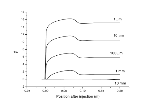
Figure 1: Radial force normalized to $e^{2}\lambda/(4\pi\varepsilon_{0}R)$, $\hat{F}$, felt by a particle with different vertical displacements $h$ positioned at the center of a line bunch $200~{}\mu m$ long as the bunch enters a circle of radius $R=1~{}m$. Here $\gamma=100$. These simulations were obtained by means of the code $TraFiC^{4}$.

The figure shows the normalized radial force (i.e. the force normalized to $e^{2}\lambda/(4\pi\varepsilon_{0}R)$ in the direction orthogonal to the test particle velocity and still lying on the bending plane) felt by a test particle. Here $\lambda$ is the bunch density while $h$ is the vertical (orthogonal to the bending plane) displacement with respect to the center of a one-dimensional bunch with rectangular density distribution function.

The plot shows interesting characteristics: a very sharp feature at the injection position, a transient and a steady state, which we can observe but for which there is no intuitive physical explanation. The electromagnetic problem is, of course, only a part of the formidable evolution problem but its understanding is $perse$ an important physical issue.

Analytical investigations of this simplified, although very important situation are therefore needed in order to see the meaning of the simulation results, besides providing, from a more practical viewpoint, important cross-checks. We will show that through this kind of study we can understand the features of Fig. 1 from a physical viewpoint, deal with characteristic times and lengths and, as a very practical result, validate the simulation results by producing analytical cross-checks.

The self-interaction in the longitudinal direction (parallel, at any time, to the velocity vector by definition) is responsible for the energy exchange between the system and the acceleration field and for all CSR (Coherent Synchrotron Radiation)-related phenomena, which have been studied extensively elsewhere (see, amongst others, ROTH … BORL ).

Self-forces in the transverse direction were first addressed, in the case of a circular motion, and from an electrodynamical viewpoint, in TALM . Further analysis (RUI2 , LEE … STUP ) considers, again, the case of circular motion both from an electrodynamical and a dynamical viewpoint. We proposed a fully electrodynamical analysis of a bunch moving in an arc of a circle in OURS , where, for the reasons explained before, we were not interested in the full evolution problem. Nevertheless, in that paper we addressed the issue of understanding the electromagnetic interactions only in the framework of a 1D model. Before our study in OURS there was no explanation for the simulation results shown in Fig. 1. The work in OURS provided a qualitative explanation of these results: such qualitative character of the explanation is due to the fact that the model in OURS is one-dimensional, and does not allow any quantitative investigation when (as in Fig. 1) a vertical displacement is introduced. Still it was possible to demonstrate that the sharp feature near the injection point is due to interactions of the test particle with particles in front of it, while the transient part is due to the interaction with particles behind it.

In this paper we aim at an extension of the model proposed in OURS which allows a fully electrodynamical analysis of a bunch endowed with a vertical dimension. Since a bunch with vertical extent can be always thought of as a superposition of displaced charge lines, all the relevant physical aspects of the problem are included in the study of a simpler model, constituted by a one-dimensional line bunch and a test particle with vertical displacement, which is the situation studied in Fig. 1. In this article, our explanation of the features in Fig. 1 will be eventually refined to a quantitative level.

The paper is organized as follows. We first treat, in Section II, the transverse interaction between two particles moving in an arc of a circle, supposing that one of the two particles has a vertical displacement $h$ with respect to the source. By integration of our results we consider, in Section III, a stepped-profile electron bunch interacting with a test particle with vertical displacement entering an arc of a circle and we discuss all the characteristic lengths involved. Finally, in Section IV, we come to a summary of the results obtained and to conclusions.

II TRANSVERSE INTERACTION BETWEEN TWO ELECTRONS

We will first address the case of two electrons moving in an arc of a circle of radius $R$, in such a way that one of the two is displaced, with respect to the reference trajectory, by a quantity $h$ in the vertical (perpendicular to the bending plane) direction. We will see that, as concerns the interaction in the radial direction (in the bending plane) it does not matter which particle is endowed with this displacement.

The electro-magnetic force which one of the two particles (designated with ”T”, i.e. the test particle) feels, due to the interaction with the other one (designated with ”S”, i.e. the source particle), is given by

$${\bm{F}}({\bm{r_{\mathrm{T}}}},t)=e{\bm{E}}({\bm{r_{\mathrm{T}}}},t)+ec{\bm{\beta_{\mathrm{T}}}}\times{\bm{B}}({\bm{r_{\mathrm{T}}}},t),$$ (3)

where ${\bm{r_{\mathrm{T}}}}$ is the position of the test particle, $e$ is the electron charge with its own (negative) sign, $\bm{\beta_{\mathrm{T}}}$ is the velocity of the test particle normalized to the speed of light, $c$, while $\bm{E}({\bm{r_{\mathrm{T}}}},t)$ and $\bm{B}({\bm{r_{\mathrm{T}}}},t)$ are, respectively, the electric and the magnetic field generated at a given time $t$ by the source particle S, at the position of the test particle T, namely

$${\bm{E}}({\bm{r_{\mathrm{T}}}},t)={e\over{4\pi\varepsilon_{\mathrm{0}}}}\Biggl{\{}{1\over\gamma_{\mathrm{S}}^{2}}{{\bf{\hat{n}}}-{\bm{\beta_{\mathrm{S}}}}\over{R_{\mathrm{ST}}^{2}\left({1-{\bf{\hat{n}}}\cdot{\bm{\beta_{\mathrm{S}}}}}\right)^{3}}}+$$

(4)

$$+{1\over c}{{\bf{\hat{n}}}\times\left[{\left({{\bf{\hat{n}}}-{\bm{\beta_{\mathrm{S}}}}}\right)\times{\dot{\bm{\beta}}_{\bm{\mathrm{S}}}}}\right]\over{R_{\mathrm{ST}}\left({1-{\bf{\hat{n}}}\cdot{\bm{\beta_{\mathrm{S}}}}}\right)^{3}}}\Biggr{\}}~{}$$ (5)

and

$${\bm{B}}({\bm{r_{\mathrm{T}}}},t)={1\over c}{\bf{\hat{n}}}\times{\bm{E}}({\bm{r_{\mathrm{T}}}},t)~{}.$$ (6)

Here ${\bm{\beta_{\mathrm{S}}}}$ and ${\dot{\bm{\beta}}_{\bm{\mathrm{S}}}}$ are, respectively, the dimensionless velocity and its time derivative at the retarded time $t^{\prime}$, $R_{\mathrm{ST}}$ is the distance between the retarded position of the source particle and the present position of the test electron, $\bf{\hat{n}}$ is a unit vector along the line connecting those two points and $\gamma_{\mathrm{S}}$ is the usual Lorentz factor referred to the source particle at the retarded time $t^{\prime}$.

In contrast to the case studied in OURS , the transverse (by definition, orthogonal to ${\bm{\beta_{\mathrm{T}}}}$) projection of ${\bm{F}}({\bm{r_{\mathrm{T}}}},t)$ has now components both in the bending plane and perpendicular to it. We will introduce, therefore, two unit vectors $\bf{\hat{e}_{h}}$, in the direction perpendicular to the bending plane, and $\bf{\hat{e}_{p}}$, in the radial direction, i.e. orthogonal to $\bm{\beta_{\mathrm{T}}}$ and lying in the bending plane. Of course, the transverse component of ${\bm{F}}({\bm{r_{\mathrm{T}}}},t)$ can still be written, following OURS , as the sum of contributions from the velocity (”C”, Coulomb) and the acceleration (”R”, Radiation) fields, namely

$${\bm{F_{\bot}}}({\bm{{r_{\mathrm{T}}}}},t)={\bm{F_{\mathrm{\bot C}}}}({\bm{r_{\mathrm{T}}}},t)+{\bm{F_{\mathrm{\bot R}}}}({\bm{r_{\mathrm{T}}}},t),$$ (7)

where

$${\bm{F}_{\bm{\mathrm{\bot C}}}}({\bm{r_{\mathrm{T}}}},t)={e^{2}\over{4\pi\varepsilon_{\mathrm{0}}}}{{\bf{n_{\bot}}}\left(1-{\bm{\beta_{\mathrm{S}}}}\cdot{\bm{\beta_{\mathrm{T}}}}\right)-{\bm{\beta_{\mathrm{\bot S}}}}\left(1-{\bf{\hat{n}}}\cdot{\bm{\beta_{\mathrm{T}}}}\right)\over{\gamma_{\mathrm{S}}^{2}R_{\mathrm{ST}}^{2}\left(1-{\bf{\hat{n}}}\cdot{\bm{\beta_{\mathrm{S}}}}\right)^{3}}}$$ (8)

and

$${\bm{F}_{\bm{\mathrm{\bot R}}}}({\bm{r_{\mathrm{T}}}},t)={e^{2}\over{4\pi\varepsilon_{\mathrm{0}}}}\times$$ (9)

$$\times\Bigg{[}{{\bf{n_{\bot}}}\left({\bf{\hat{n}}}\cdot{{\dot{\bm{\beta}}_{\bm{\mathrm{S}}}}}\right)\left(1-{\bm{\beta_{\mathrm{S}}}}\cdot{\bm{\beta_{\mathrm{T}}}}\right)-{\bm{\beta_{\mathrm{\perp S}}}}\left({\bf{\hat{n}}}\cdot{{\dot{\bm{\beta}}_{\bm{\mathrm{S}}}}}\right)\left(1-{\bf{\hat{n}}}\cdot{\bm{\beta_{\mathrm{T}}}}\right)\over{R_{\mathrm{ST}}\left(1-{\bf{\hat{n}}}\cdot{\bm{\beta_{\mathrm{S}}}}\right)^{3}}}-{\dot{\bm{\beta}}_{\bm{\mathrm{\perp T}}}\left(1-{\bf{\hat{n}}}\cdot{\bm{\beta_{\mathrm{T}}}}\right)+{\bf{\hat{n}_{\perp}}}\left({\bm{\beta_{\mathrm{T}}}}\cdot{{\dot{\bm{\beta}}_{\bm{\mathrm{S}}}}}\right)\over{R_{\mathrm{ST}}\left(1-{\bf{\hat{n}}}\cdot{\bm{\beta_{\mathrm{S}}}}\right)^{2}}}\Bigg{]}\;$$ . (10)

II.1 Tail-Head interaction: case of two particles in circular motion

We will first consider the situation in which the test particle is in front of the source. In this case, one can refer to Fig. 2 for all the possible configurations of the present position of the test electron and the retarded position of the source with respect to the arc. The vertical displacement $h$ of one of the two particles is to be imagined in the direction perpendicular to the figure plane. Let us start with the steady state case in Fig. 2b. We can define with $\Delta s$ the curvilinear distance between the present position of the test and of the source particle; $\phi$ will indicate the angular distance between the retarded position of the source and the present position of the test electron, and it will be designated as the retarded angle. Finally, $h$ will be the vertical displacement.

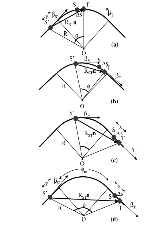
Figure 2: Relative configuration of the retarded source point S’ and the test point T for a system of two electron passing a bending magnet. The test particle is understood to be displaced by a quantity $h$ in the vertical direction. The figure shows only the projection of the motion on the bending plane.

In the following we will assume $\beta_{\mathrm{S}}=\beta_{\mathrm{T}}=\beta$. Therefore we can write Eq. (8) and Eq. (10) in the following way:

$${\bm{F_{\mathrm{\bot C}}}}={e^{2}\over{4\pi\varepsilon_{\mathrm{0}}}\gamma^{2}}{{{\bf{\hat{e}_{h}}}\left[h(1-\beta^{2}\cos\phi)\right]+{\bf{\hat{e}_{p}}}\left[2R\sin^{2}(\phi/2)(1+\beta^{2})-\beta\sin\phi(h^{2}+4R^{2}\sin^{2}(\phi/2))^{1/2}\right]}\over{\left[(h^{2}+4R^{2}\sin^{2}(\phi/2))^{1/2}-2\beta R\sin(\phi/2)\cos(\phi/2)\right]^{3}}}~{},$$ (11)

$${\bm{F_{\mathrm{\bot R}}}}={e^{2}\beta^{2}c\over{4\pi\varepsilon_{\mathrm{0}}}}\times$$ (12)

$$\times\Bigg{\{}2\sin^{2}(\phi/2){{\bf{\hat{e}_{h}}}\left[h(1-\beta^{2}\cos\phi)\right]+{2{\bf{\hat{e}_{p}}}\sin(\phi/2)\left[R\sin(\phi/2)(1+\beta^{2})-\beta\cos(\phi/2)(h^{2}+4R^{2}\sin^{2}(\phi/2))^{1/2}\right]}\over{\left[(h^{2}+4R^{2}\sin^{2}(\phi/2))^{1/2}-2\beta R\sin(\phi/2)\cos(\phi/2)\right]^{3}}}-$$ (13)

$$-{{\bf{\hat{e}_{h}}}\left[h\beta\sin\phi\right]+{\bf{\hat{e}_{p}}}\left[\beta R\sin\phi-\cos\phi(h^{2}+4R^{2}\sin^{2}(\phi/2))^{1/2}\right]\over{R\left[(h^{2}+4R^{2}\sin^{2}(\phi/2))^{1/2}-2\beta R\sin(\phi/2)\cos(\phi/2)\right]^{2}}}\Bigg{\}}~{}.$$ (14)

The retardation condition linking $\Delta s$, $h$ and $\phi$ reads

$$\Delta s=R\phi-\beta\left[h^{2}+4R^{2}\sin^{2}{\phi\over{2}}\right]^{1/2}~{},$$ (15)

As one can readily see by inspecting Eq. (15), when we impose reasonable values for $\Delta s\ll R$ and $h\ll R$ we obtain corresponding values of $\phi\ll 1$. We will therefore assume $\phi\ll 1$ throughout this paper, and verify $a~{}posteriori$ the validity of this assumption when studying particular situations. Note that, by fixing $\phi\ll 1$ we keep open the possibility of comparing $\phi$ with the synchrotron radiation formation angle $1/\gamma$ (note that a deflection angle smaller or larger than $1/\gamma$ is characteristic of the cases, respectively, of undulator or synchrotron radiation). We can therefore expand Eq. (11) and Eq. (14) to the second non-vanishing order in $\phi$ thus obtaining

$${\bm{F_{\mathrm{\bot C}}}}\simeq{e^{2}\gamma^{3}\over{4\pi\varepsilon_{\mathrm{0}}R^{2}}}{\bm{\Phi_{\mathrm{C}}}}(\hat{\phi})$$ (16)

and

$${\bm{F_{\mathrm{\bot R}}}}\simeq{e^{2}\gamma^{3}\over{4\pi\varepsilon_{\mathrm{0}}R^{2}}}{\bm{\Phi_{\mathrm{R}}}}(\hat{\phi})~{},$$ (17)

where we define ${\bm{\Phi_{\mathrm{C}}}}$ and ${\bm{\Phi_{\mathrm{R}}}}$ as

$${\bm{\Phi_{\mathrm{C}}}}(\hat{\phi})={{4{\bf{\hat{e}_{h}}}\left[\hat{h}+2\hat{h}/\hat{\phi}^{2}\right]+{\bf{\hat{e}_{p}}}\left[\hat{\phi}^{2}-4\hat{h}^{2}/\hat{\phi}^{2}\right]}\over{\hat{\phi}\left[1+\hat{\phi}^{2}/4+\hat{h}^{2}/\hat{\phi}^{2}\right]^{3}}}$$ (18)

and

$${\bm{\Phi_{\mathrm{R}}}}(\hat{\phi})={{{\bf{\hat{e}_{h}}}\hat{\phi}^{2}\hat{h}\left[1-4\hat{h}^{2}/\hat{\phi}^{4}\right]+{\bf{\hat{e}_{p}}}\left[2-\hat{\phi}^{2}-3\hat{h}^{2}+4\hat{h}^{2}/\hat{\phi}^{2}\right]}\over{\hat{\phi}\left[1+\hat{\phi}^{2}/4+\hat{h}^{2}/\hat{\phi}^{2}\right]^{3}}}$$ (19)

Here and above $\hat{\phi}=\gamma\phi$. This normalization choice, already treated in SALLONG , is quite natural, $1/\gamma$ being the synchrotron radiation formation-angle at the critical wavelength. In the derivation of Eq. (16) and Eq. (17) (and in the following, too) we understood $\hat{\phi}\gg 1/\gamma$, which is justified by the ultrarelativistic approximation. Moreover we defined $\hat{h}=h\gamma^{2}/R$; in order to understand this definition we first write down the retardation condition Eq. (15) in approximate form. Since we are already working in the limit $\Delta s/R\ll 1$ and $\phi\ll 1$, then in order to have $\Delta s>0$, $h<R\phi$ must be satisfied. We will automatically recover from our results that the assumption $h\ll R\phi$ is sufficiently good for our purposes. Therefore Eq. (15) can be approximated with:

$$\Delta s=(1-\beta)R\phi+{R\phi^{3}\over{24}}-{\beta h^{2}\over{2R\phi}}~{}.$$ (20)

The latter can be written down in dimensionless form too as

$$\Delta\hat{s}={\hat{\phi}\over{2}}+{\hat{\phi}^{3}\over{24}}-{\hat{h}^{2}\over{2\hat{\phi}}}~{},$$ (21)

which explains the choice of the definition for $\hat{h}$.

The reader may easily check that Eq. (18), Eq. (19) and Eq. (21) (as well as Eq. (11) and Eq. (14)) are generalizations of the expressions given in OURS by taking their limit for $\hat{h}\longrightarrow 0$.

The following expression, which is valid for the total transverse force felt by the test particle can be then trivially derived

$${\bm{F_{\mathrm{\bot}}}}\simeq{e^{2}\gamma^{3}\over{4\pi\varepsilon_{\mathrm{0}}R^{2}}}{\bm{\Phi}}(\hat{\phi})~{},$$ (22)

where $\Phi$ is defined by

$${\bm{\Phi}}(\hat{\phi})={\bm{\Phi_{\mathrm{R}}}}(\hat{\phi})+{\bm{\Phi_{\mathrm{C}}}}(\hat{\phi}),$$ (23)

II.2 Tail-Head interaction: case (a)

Let us now consider the other cases depicted in Fig. 2a, c and d. While the case in Fig. 2b deals with the steady state situation in which the present position of the test and the retarded position of the source are both in the bend, Fig. 2a, c and d deal with transient situations in which we can find the retarded source and the present test in the straight line before and after the bend too.

Consider the situation in Fig. 2a. In this case, under the assumption $h\ll(y+R\phi)$, the retardation condition reads

$$\Delta\hat{s}\simeq{\hat{y}+\hat{\phi}\over{2}}-{1\over{2}}{\hat{h}^{2}-\hat{\phi}^{3}/3(\hat{y}+\hat{\phi}/4)\over{\hat{y}+\hat{\phi}}}~{},$$ (24)

where we introduced the normalized quantity $\hat{y}=y\gamma/R$, which is just $y/R$ normalized to the synchrotron radiation formation angle, $1/\gamma$.

In this case the source particle is only responsible for a velocity field contribution, therefore ${\bm{F}_{\mathrm{\bot}}}={\bm{F}_{\mathrm{\bot C}}}$. By direct use of Eq. (8), one can find the exact expression for ${\bm{F}_{\mathrm{\bot}}}$

$${\bm{F}_{\mathrm{\bot}}}={e^{2}\over{4\pi\varepsilon_{\mathrm{0}}\gamma^{2}}}{{{\bf{\hat{e}_{h}}}\left\{h[1-\beta^{2}\cos\phi]\right\}+{\bf{\hat{e}_{p}}}\left\{-R_{ST}\beta\sin\phi+\left[R(1+\beta^{2})(1-\cos\phi)+y\sin\phi\right]\right\}}\over{\left\{R_{ST}-\beta(y+R\sin\phi)\right\}^{3}}}$$ (25)

$R_{ST}$ being given by

$$R_{ST}=\left[(y+R\sin\phi)^{2}+R^{2}(1-\cos\phi)^{2}+h^{2}\right]^{1/2}~{}.$$ (26)

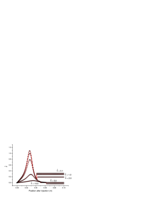
Figure 3: Normalized radial force $\hat{F}$ for a two-particle system entering a hard-edge bending magnet as a function of the position after injection. Results for different values of $\hat{h}$ are shown. The solid lines show analytical results; the circles describe the outcome from $\mathrm{TRAFIC}^{4}$. Here $\Delta\hat{s}=5.0$.

Expanding the trigonometric functions in Eq. (25) and using normalized quantities one finds:

$${\bm{F}_{\mathrm{\bot}}}\simeq{e^{2}\over{4\pi\varepsilon_{\mathrm{0}}}}{4\gamma^{3}\over{R^{2}}}(\hat{y}+\hat{\phi})^{2}{\left\{{\bf{\hat{e}_{h}}}\left[\hat{h}(\hat{y}+\hat{\phi})(2+\hat{\phi}^{2})\right]+{\bf{\hat{e}_{p}}}\left[\hat{y}^{2}\phi+\hat{y}(\hat{\phi}^{2}+\hat{\phi}^{4}/2)+{\hat{\phi}^{5}/4}-\hat{h}^{2}\phi\right]\right\}\over{\left[(\hat{y}+\hat{\phi})^{2}+{\hat{\phi}^{4}/4}+\hat{h}^{2}\right]^{3}}}$$ (27)

It can be easily verified that, as it must be, Eq. (27) reduces to Eq. (16) in the limit $\hat{y}\rightarrow 0$. Also, the reader may check that in the limit $\hat{h}\rightarrow 0$, Eq. (27) reduces to already derived expressions in OURS .

Let us now define the normalized radial force $\hat{F}=F_{p}/[e^{2}/(4\pi\varepsilon_{0}R\Delta s)]$. It is possible, by means of Eq. (27), to plot $\hat{F}$ as a function of the position after the injection (defined by the entrance of the test particle in the hard-edge magnet) for a fixed value of $\Delta\hat{s}=\Delta s\gamma^{3}/R=5.0$ and different values of $h$. In Fig. 3 we compare such a plot with numerical results from the code $\mathrm{TRAFIC}^{4}$ (see ROTH ).

Note that, as already pointed out in OURS , at the position which corresponds to the entrance of the retarded source in the magnet there is a discontinuity in the plots. This is linked to our model choice, and it is due to the abrupt (hard edge magnet) switching on of the acceleration fields.

As general remark to Fig. 3 and, in fact to Fig. 4, 6 and Fig.11, the perfect agreement between our calculations and numerical results by $\mathrm{TRAFIC}^{4}$ provides, per se, an excellent cross-check between our analytical results (with their assumptions and applicability region) and simulations.

II.3 Tail-Head interaction: case (c)

We will now move to the case depicted in Fig. 2c, in which the source particle has its retarded position inside the bend and the test particle has its present position in the straight line following the magnet. We will define with $x$ the distance, along the straight line after the magnet, between the end of the bend and the present position of the test particle. Here $\hat{\phi}_{\mathrm{m}}=\gamma\phi_{\mathrm{m}}$, $\phi_{\mathrm{m}}$ being the angular extension of magnet, and $\hat{x}=\gamma x/R$, the reason for this normalization choice for $x$ being identical to that for $y$.

The retardation condition reads

$$\Delta\hat{s}\simeq{\hat{\psi}+\hat{x}\over{2}}+{\hat{\psi}^{3}\over{24}}{\hat{\psi}+4\hat{x}\over{\hat{\psi}+\hat{x}}}-{\hat{h}^{2}\over{2(\hat{\psi}+\hat{x})}}.$$ (28)

In contrast with the case of Fig. 2a, here we have contributions from both velocity and acceleration field. Again, by direct use of Eq. (8) and Eq. (10) one can find the exact expression for the transverse electromagnetic force exerted by the source particle on the test particle

$${\bm{F}_{\mathrm{\bot}}}={\bm{F}_{\mathrm{\bot C}}}+{\bm{F}_{\mathrm{\bot R}}}~{},$$ (29)

where

$${\bm{F}_{\mathrm{\bot C}}}={e^{2}\over{4\pi\varepsilon_{\mathrm{0}}\gamma^{2}}}{{\bf{\hat{e}_{h}}}\left[(1-\beta^{2}\cos\psi)h\right]+{\bf{\hat{e}_{p}}}\left[R(1-\cos\psi)(1-\beta^{2}\cos\psi)-\beta\sin\psi\left(R_{ST}-\beta x-\beta R\sin\psi\right)\right]\over{\left[R_{ST}-\beta x\cos\psi-\beta R\sin\psi\right]^{3}}}~{}$$ (30)

and

$${\bm{F}_{\mathrm{\bot R}}}={e^{2}\over{4\pi\varepsilon_{\mathrm{0}}R}}\Bigg{\{}\Bigg{[}{{{\bf{\hat{e}_{h}}}\left[\beta^{2}h(1-\beta^{2}\cos\psi)(R+x\sin\psi-R\cos\psi)\right]}\over{\left[R_{ST}-\beta x\cos\psi-\beta R\sin\psi\right]^{3}}}+$$ (31)

$$+{{{\bf{\hat{e}_{p}}}\beta^{2}\left[(R+x\sin\psi-R\cos\psi)(R(1-\cos\psi)(1-\beta^{2}\cos\psi)-\beta\sin\psi(R_{ST}-\beta x+\beta R\sin\psi))\right]}\over{\left[R_{ST}-\beta x\cos\psi-\beta R\sin\psi\right]^{3}}}\Bigg{]}-$$ (32)

$$-{{\bf{\hat{e}_{h}}}\beta^{2}\left[h\sin\psi\right]+{\bf{\hat{e}_{p}}}\left[R(1-\cos\psi)\beta^{2}\sin\psi-\beta\cos\psi(R_{ST}-\beta x-\beta R\sin\psi)\right]\over{\left[R_{ST}-\beta x\cos\psi-\beta R\sin\psi\right]^{2}}}\Bigg{\}} ~{}.$$ (33)

$R_{ST}$ being now

$$R_{ST}=\left((x+R\sin\psi)^{2}+R^{2}(1-\cos\psi)^{2}+h^{2}\right)^{1/2}$$ (34)

Expanding the trigonometric functions in Eq. (30) and Eq. (33), and using normalized quantities one finds:

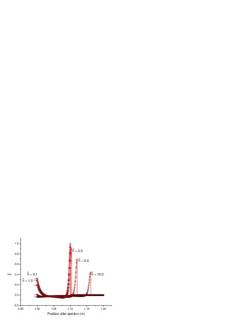
Figure 4: Normalized radial force $\hat{F}$ for a two-particle system leaving a hard-edge bending magnet as a function of the position after the ejection. Results for different values of $\hat{h}$ are shown. The solid lines show analytical results; the circles describe the outcome from $\mathrm{TRAFIC}^{4}$. Here $\Delta\hat{s}=5.0$.

$${\bm{F}_{\mathrm{\bot C}}}={2e^{2}\gamma^{3}\over{4\pi\varepsilon_{\mathrm{0}}R^{2}}}{2{\bf{\hat{e}_{h}}}\left[\hat{h}(2+\hat{\psi}^{2})(\hat{x}+\hat{\psi})^{3}\right]+{\bf{\hat{e}_{p}}}\hat{\psi}(\hat{x}+\hat{\psi})^{2}\left[-2\hat{x}^{2}+\hat{x}\left(\hat{\psi}^{3}-2\hat{\psi}\right)+{\hat{\psi}^{4}/2}-2\hat{h}^{2}\right]\over{\left[(\hat{x}+\hat{\psi})^{2}+({\hat{\psi}^{2}/4})(2\hat{x}+\hat{\psi})^{2}+\hat{h}^{2}\right]^{3}}}~{},$$ (35)

and

$${\bm{F}_{\mathrm{\bot R}}}={2e^{2}\gamma^{3}\over{4\pi\varepsilon_{\mathrm{0}}R^{2}}}(\hat{x}+\hat{\psi})\Bigg{\{}{-2{\bf{\hat{e}_{h}}}\left[\hat{h}\hat{\psi}(\hat{x}+\hat{\psi})\right]+{\bf{\hat{e}_{p}}}\left[\hat{x}^{2}+\hat{x}\hat{\psi}(2-\hat{\psi}^{2})+\hat{\psi}^{2}-(3/4)\hat{\psi}^{4}+\hat{h}^{2}\right]\over{\left[(\hat{x}+\hat{\psi})^{2}+(\hat{\psi}^{2}/4)(2\hat{x}+\hat{\psi})^{2}+\hat{h}^{2}\right]^{2}}}+$$ (36)

$$+{2{{\bf{\hat{e}_{h}}}(\hat{x}+\hat{\psi})^{2}(2+\hat{\psi}^{2})(\hat{x}+\hat{\psi}/2)\hat{\psi}\hat{h}+{\bf{\hat{e}_{p}}}(\hat{x}+\hat{\psi})(\hat{x}+\hat{\psi}/2)\hat{\psi}^{2}\big{[}-2\hat{h}^{2}-2\hat{x}^{2}+\hat{x}\hat{\psi}(-2+\hat{\psi^{2}})+\hat{\psi}^{4}/2\big{]}}\over{\left[(\hat{x}+\hat{\psi})^{2}+(\hat{\psi}^{2}/4)(2\hat{x}+\hat{\psi})^{2}+\hat{h}^{2}\right]^{3}}}\Bigg{\}}$$ (37)

Similarly to the latter case, it can be easily verified that Eq. (35) and Eq. (37) reduce to Eq. (16) and Eq. (17), respectively, in the limit $x\rightarrow 0$. Moreover, in the limit $h\rightarrow 0$, they reduce to already known expressions given in OURS . Again, one can plot the normalized radial force $\hat{F}$ as a function of the position after the ejection, defined by the exit of the test particle from the hard-edge magnet, for different values of $\hat{h}$ and a fixed value of $\Delta\hat{s}=\Delta s\gamma^{3}/R=5.0$. In Fig. 4 we compare such a plot with numerical results from $\mathrm{TRAFIC}^{4}$.

At the position which corresponds to the exit of the retarded source from the magnet there is a discontinuity in the plots. This, again, is linked to our model choice, and it is due to the fact that, for particles on axis, after the retarded source has left the magnet there is only Coulomb repulsion along the longitudinal direction.

Figure 5: Time variation of a synchrotron radiation pulse generated by a highly relativistic electron moving in a circle as seen by an observer in the orbital plane

It is suggestive to notice the resemblance of the peaks shown in Fig. 4 with half of the time pulse of the radial electric field from usual synchrotron radiation process (see Fig. 5, and DIAGN ). This is not a coincidence. The test particle is, indeed, far away from the source with respect to the formation length $R/\gamma^{3}$ and the magnetic field contribution to the Lorentz force can be expected to have the same behavior of the electric field contribution, since ${\bm{B}}=({\bf{\hat{n}}}\times{\bm{E}})/c$. The only difference is that the observer is now ”running away” from the electromagnetic signal which will result in a spreading of the pulse of about a factor $(1-\beta)^{-1}$. Since $R=1~{}m$ and $\gamma=100$ we expect the pulse to be long about $(R/\gamma^{3})(1-\beta)^{-1}\sim 10^{-2}~{}m$.

II.4 Tail-Head interaction: case (d)

The last Tail-Head case left to discuss is depicted in Fig. 2d; the source particle has its retarded position in the straight line before the bend, and the test particle has its present position in the straight line following the magnet. The retardation condition reads

$$\Delta\hat{s}\simeq{\hat{\phi}_{\mathrm{m}}+\hat{x}+\hat{y}\over{2}}+$$ (38)

$$+{\hat{\phi}_{\mathrm{m}}^{3}/{24}\left[\hat{\phi}_{\mathrm{m}}+4(\hat{x}+\hat{y})+12\hat{x}\hat{y}/\hat{\phi}_{\mathrm{m}}\right]-\hat{h}^{2}/2\over{\hat{\phi}_{\mathrm{m}}+\hat{x}+\hat{y}}}$$ . (39)

In this case we have only velocity contributions. The exact expression for the electromagnetic transverse force on the test particle is

$${\bm{F}_{\mathrm{\bot}}}={e^{2}\over{4\pi\varepsilon_{\mathrm{0}}\gamma^{2}}}{{\bf{\hat{e}_{h}}}\left[\sin\theta(1-\beta^{2}\cos\phi_{m})\right]+{\bf{\hat{e}_{p}}}\left[\sin\delta\cos\theta(1-\beta^{2}\cos\phi_{m})-\beta\sin\phi_{m}(1-\cos\delta\cos\theta)\right]\over{R_{ST}^{2}\left[1-\beta\sin\phi_{m}\sin\delta\cos\theta-\beta\cos\phi_{m}\cos\delta\cos\theta\right]^{3}}}$$ (40)

where

$$\sin\theta={h\over{R_{ST}}}~{},$$ (41)

$$\cos\theta={(R_{ST}^{2}-h^{2})^{1/2}\over{R_{ST}}}~{},$$ (42)

$$\sin\delta={R+y\sin\phi_{m}-R\cos\phi_{m}\over{R_{ST}\cos\theta}}~{},$$ (43)

and

$$\cos\delta={x+y\cos\phi_{m}+R\sin\phi_{m}\over{R_{ST}\cos\theta}}~{},$$ (44)

where $R_{ST}$ can be retrieved by the latter two equations and some trivial trigonometry.

Once again, expanding the trigonometric functions in Eqs. (40) … (43) and using normalized quantities one finds the following approximated expression for ${\bm{F}_{\mathrm{\bot}}}$:

$${\bm{F}_{\mathrm{\bot}}}\simeq{e^{2}\over{4\pi\varepsilon_{\mathrm{0}}R^{2}}}4\gamma^{3}(\hat{x}+\hat{y}+\hat{\phi}_{\mathrm{m}})^{2}\hat{\phi}_{\mathrm{m}}\times$$

$$\times{{\bf{\hat{e}_{h}}}\left[({2/{\hat{\phi}_{m}}}+{\hat{\phi}_{m}})(\hat{x}+\hat{y}+\hat{\phi}_{m})\hat{h}\right]+{\bf{\hat{e}_{p}}}\left[-{\hat{x}^{2}}+{\hat{y}^{2}}+({\hat{\phi}_{\mathrm{m}}^{2}})\hat{x}\hat{y}+{\hat{x}(\hat{\phi}_{\mathrm{m}}^{3}/2-\hat{\phi}_{\mathrm{m}})}+{\hat{y}(\hat{\phi}_{\mathrm{m}}^{3}/2+\hat{\phi}_{\mathrm{m}})}+{\hat{\phi}_{\mathrm{m}}^{4}/4}-\hat{h}^{2}\right]\over{\left\{(\hat{x}+\hat{y}+\hat{\phi}_{\mathrm{m}})\left[\hat{x}(1+\hat{\phi}^{2}_{\mathrm{m}})+\hat{y}+\hat{\phi}_{\mathrm{m}}+{\hat{\phi}^{3}_{\mathrm{m}}/3}\right]-(\hat{\phi}^{2}_{\mathrm{m}}/12)[12\hat{x}\hat{y}+4(\hat{x}+\hat{y})\hat{\phi}_{\mathrm{m}}+\hat{\phi}_{\mathrm{m}}^{2}]+\hat{h}^{2}\right\}^{3}}}~{}.$$ (46)

It is easy to verify that Eq. (46) reduces, respectively, to the steady state (Eq. (16)) when $x=0$ and $y=0$, to the transient case in Fig. 2a when $x=0$ (Eq. (27)) and to the transient case in Fig. 2c when $y=0$ (Eq. (30)). Moreover the reader may verify that, in the limit $h\longrightarrow 0$, Eq. (46) reduces to already known results in OURS . Following the treatment of the transient situations in Fig. 2a and in Fig. 2c we plot, for this case too, a normalized expression for the transient force, i.e. the usual $\hat{F}$, as a function of the curvilinear position of the test particle ($s=0$ indicates the entrance of the magnet) for different values of $\hat{h}$ and a fixed value of $\Delta\hat{s}=\Delta s\gamma^{3}/R$ and magnet length. In Fig. 6, we compare our analytical results with numerical results from $\mathrm{TRAFIC}^{4}$, for a fixed value of $\Delta\hat{s}=5.0$ and $\hat{\phi}_{m}=1$ and for different values of the vertical displacement $\hat{h}$.

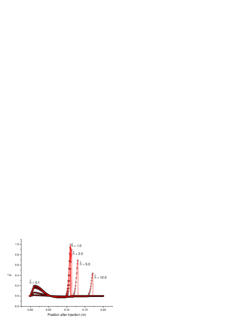
Figure 6: Normalized radial force $\hat{F}$ for a two-particle system crossing a hard-edge bending magnet as a function of the position of the test particle inside the magnet in the case of a short magnet ${\phi}_{\mathrm{m}}\ll 1$. Results are shown for different values of $\hat{h}$. The solid lines show analytical results; the circles describe the outcome from $\mathrm{TRAFIC}^{4}$. Here the normalized distance between the two particles is $\Delta\hat{s}=5$, while $\hat{\phi}_{m}=1$.

II.5 Head-Tail interaction

Finally, we can deal with the situation in which the source particle is ahead of the test electron, i.e. $\Delta s<0$; we will talk, in this case, of head-tail interaction. On the one hand it is evident that, when $\Delta s<0$, the source particle is ahead of the test electron at any time; on the other hand it is not true that the present position of the test particle is, in general, ahead of the retarded position of the test particle. As already suggested in OURS , if $\Delta s<0$ and, approximatively, $|\Delta s|<h$ the test particle overtakes the retarded position of the source before the electromagnetic signal reaches it. In this case, although we may still talk about head-tail interaction, since $\Delta s<0$, its real character is very much similar to the case $\Delta s>0$, just treated in the previous subsections, in which the electromagnetic signal has to catch up with the test particle. In order to understand the physics involved in this situation it is sufficient to study the cases $\Delta s<0$ and $|\Delta s|>h$. The case $\Delta s<0$ with $|\Delta s|<h$ will be treated from a qualitative viewpoint only: its quantitative analysis, which may be interesting to perform for the sake of completeness, presents stronger mathematical difficulties and is left for future study. Anyway a qualitative treatment of this situation is enough to reach a full understanding of the interaction physics, which is our goal here.

Consider therefore the case $\Delta s<0$ with $|\Delta s|>h$. It is important to note that, once the steady state case is studied, the situation in which the source particle is ahead of the test electron can be treated immediately for all three (a, c and d) transient cases in Fig. 2 (of course, with respect to the figure, test and source particle exchange roles) on the basis of the steady state case alone. In fact in that situation, as it has already been said in OURS , we can assume the retarded angle $\phi$ small enough (the test particle ”runs against” the electromagnetic signal) that the actual trajectory followed by the particles is not essential and one can use the steady state expression to describe also the transient cases. It can be shown that the only important contribution from the source particle comes from the acceleration part of the Lienard-Wiechert fields. Within our approximations, the only non-negligible contribution is present in the situation (again, with the roles of test and source particle inverted) depicted in Fig. 2a and Fig. 2b, the latter just being the steady state case.

Let us deal with the steady state case of head-tail interaction in the case $|\Delta s|>h$. As already discussed in OURS , the difference with respect to the situation in which the test electron is in front of the source is that the test electron ”runs against” the electromagnetic signal emitted by the source, while in the other case it just ”runs away” from it. Therefore the relative velocity between the signal and the test electron is equal to $(1+\beta)c$, instead of $(1-\beta)c$ as in the other situation. Hence the retardation condition reads

$$\Delta s\simeq R\phi+\beta\left[R^{2}\phi^{2}+h^{2}\right]^{1/2}$$ (47)

or, solved for $\hat{\phi}$,

$$\hat{\phi}\simeq\Delta\hat{s}-\left[\Delta\hat{s}^{2}\left(1-{1\over{\gamma^{2}}}\right)-\hat{h}^{2}\right]^{1/2}~{}.$$ (48)

Note that, in the asymptotic for $\Delta\hat{s}\gg\gamma\hat{h}$ we recover the result in OURS for the one-dimensional case.

In the general case, $\bm{\beta_{\mathrm{S}}}$ is almost parallel to (and equal to) $\bm{\beta_{\mathrm{T}}}$ and antiparallel to the projection of $\bf{\hat{n}}$ on the bending plane: it turns out that the only important contribution to the radial force on the orbital plane is given by the second term on the right side of Eq. (10), and it is easy to check that

$${F_{\mathrm{\bot}}}\simeq{e^{2}\over{4\pi\varepsilon_{\mathrm{0}}R\Delta s}}~{}.$$ (49)

It may be worthwhile to underline that the force in Eq. (49) is, structurally, identical to the result in OURS although, of course, $\Delta s$ is now a function of $h$ .

III TRANSVERSE INTERACTION BETWEEN AN ELECTRON AND A BUNCH ENTERING A BEND FROM A STRAIGHT PATH

In the previous Section we dealt with all the possible configurations for a two-particle system moving in an arc of a circle. Now we are ready to provide a quantitative explanation of Fig. 1.

After the discussion, in Section II, about head-tail interactions within a system with the test particle behind the source electron, one is led to the qualitative conclusion that, within an electron bunch, interactions between sources in front of the test particle and the test particle itself are important and, in general, they must be responsible, at the entrance and at the exit of the bending magnet, for sharp changes in the transverse forces acting on the test electron. The quantitative change depends, of course, on the position of the test particle inside the bunch: the extreme cases are for the test particle at the head of the bunch, where there are just interactions with electrons behind the test particle (no head-tail interactions), and for the test particle before the tail of the bunch, at a distance $|\Delta s|>h$, where all the sources are in front of it (only head-tail interactions in the regime $|\Delta s|>h$).

III.1 Head-Tail interaction

Consider now the situation in which a one-dimensional line bunch interacts with a particle positioned at the center of the line but vertically displaced by a quantity $h$. As already said we will discuss, analytically, the head-tail interaction for $|\Delta s|>h$ only. Since the trajectory followed by the bunch is not important we can simply integrate Eq. (49) and find the contribution

$${F_{\mathrm{p~{}HT}}^{\mathrm{B}}}(\phi)\simeq\Bigg{\{}\begin{array}[]{c}0~{}~{}~{}~{}~{}~{}~{}~{}~{}~{}~{}~{}~{}~{}~{}~{}~{}~{}~{}~{}~{}~{}~{}~{}~{}~{}~{}~{}~{}~{}~{}~{}~{}~{}~{}~{}~{}~{}~{}~{}~{}~{}~{}~{}~{}~{}~{}~{}~{}~{}~{}~{}~{}~{}~{}~{}~{}~{}~{}~{}\phi<0\\ e^{2}\lambda_{0}/(4\pi\varepsilon_{\mathrm{0}}R)~{}\ln\left[\Delta s_{\mathrm{max}}/(\Delta s_{\mathrm{max}}-R\phi(1+\beta))\right]~{}~{}~{}~{}~{}~{}~{}~{}0<\phi<\Phi(h,\Delta s_{\mathrm{max}})\\ e^{2}\lambda_{0}/(4\pi\varepsilon_{\mathrm{0}}R)~{}\ln[\Delta s_{\mathrm{max}}/h]~{}~{}~{}~{}~{}~{}~{}~{}~{}~{}~{}~{}~{}~{}~{}~{}~{}~{}~{}~{}~{}~{}~{}~{}~{}~{}~{}~{}~{}~{}~{}~{}~{}~{}~{}~{}\phi>\Phi(h,\beta h)\end{array}~{},$$ (50)

where ”HT” stands for ”head-tail” and $\Phi(h,\Delta s)$ is the solution, in $\phi$, of Eq. (47) at vertical displacement $h$ and longitudinal distance $\Delta s$.

When a bunch longer than the vertical displacement $h$ enters the magnet, the particles in front of the bunch will interact with the test electron following Eq. (50), which models the radial interaction on the basis of Eq. (49). Nevertheless, Eq. (49) cannot describe the situation when the sources at a distance shorter than the vertical displacement $h$ begin to interact with the test electron. As a result the head-tail interaction has two characteristic formation lengths. The first one indicates the distance that the test electron travels from the moment it is reached by the electromagnetic signal from the first particle entering the bend, till the moment it is reached by the electromagnetic signal emitted as the particle at $\Delta s=-h$ enters the bend. This is given by $L_{1}=\beta cR(\phi_{2}-\phi_{1})=\beta cR\phi_{2}$, $\phi_{2}$ and $\phi_{1}$ being the solution of Eq. (48) when $\Delta s=l_{b}/2$ and $\Delta s=\beta h$, respectively (the reader will recognize that $\phi_{1}=0$). In the limit for $h<<l_{b}/2$ Eq. (48), substituted in the expression for $L_{1}$, gives the rule of thumb $L_{1}\simeq l_{b}/4$. The second characteristic length is given by the distance that the test electron travels from the moment it is reached by the electromagnetic signal from the particle at $\Delta s=-h$ till the moment it is reached by the electromagnetic signal emitted by the particle with $\Delta s=0$ as it enters the bend. This can be estimated to be, roughly, equal to $\gamma h$, at least when $h$ is not too large. In fact, in order to know the present angular position of the test particle when $\Delta s=0$ one should solve the retardation condition in $\phi$

$$R\phi=\beta\left[h^{2}+4R^{2}\sin^{2}(\phi/2)\right]^{1/2}$$ (51)

In the limit in which $\sin(\phi/2)\simeq\phi/2$ we have $\phi\simeq\gamma h/R$ and $L_{2}\simeq\gamma h$.

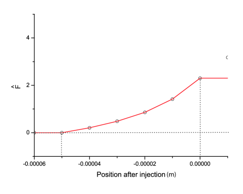
Figure 7: Normalized radial force $\hat{F}$ from the head of the bunch ($\Delta s<0$) to the tail as the bunch progresses inside the bend ($z=0$ corresponds to the injection of the test particle in the magnet). Here $R=1m,\gamma=100,h=10\mu m$ and the bunch length is $200\mu m$.The test particle is located at $\Delta s=0$.

This reasoning can explain pretty well the features in Fig. 7. The radial force grows exactly as described in Eq. (50) starting from about $z=-l_{b}/4=50~{}\mu m$ until $z=0$ (which is roughly the first formation length). Note that with the source located at $\Delta s=h$ corresponds a retarded angle $\phi=0$, which means that the electromagnetic signal from this source, which is emitted at $z=0$, will reach the test particle when this has also the position $z=0$. After $z=0$, the test particle begins to interact with the sources located at $\Delta s>-h$ while the ones at $\Delta s<-h$ reach a steady state, in the sense that they keep on interacting in the same way with the test electron.

This is illustrated by Fig. 8, where the normalized radial force $\hat{F}$ is plotted.

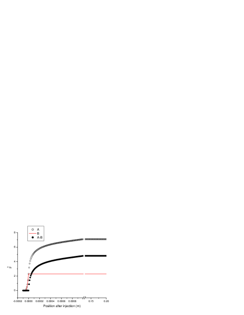
Figure 8: The same as Fig. 7 for a different range. Normalized radial force from the head of the bunch ($\Delta s<0$) to the tail as the bunch progresses inside the bend ($z=0$ corresponds to the injection of the test particle in the magnet). Here $R=1m,\gamma=100,h=10\mu m$ and the bunch length is $200\mu m$. The test particle is located at $\Delta s=0$. Curve A corresponds to the simulation by $TraFiC^{4}$, curve B is the contribution, given by Eq. 50, of the particles with $\Delta s<-h$; A-B is the difference between the two curves, ascribed to the contribution from the particles with $\Delta s>-h$.

The difference between the simulation results and the analytical estimation in Eq. (50) gives, quantitatively, the radial interaction due to the sources at $\Delta s>-h$. For $h=10~{}\mu m$ and $\gamma=100$, as in our case, one expects a second formation length equal to $10^{-3}~{}m$ which is exactly what one gets: the actual data show, in fact, that a maximum is reached when $z=0.001~{}m$ at $\hat{F}\simeq 7.098$.

Figure 9: Normalized radial force from the head of the bunch ($\Delta s<0$) to the tail as the bunch progresses inside the bend ($z=0$ corresponds to the injection of the test particle in the magnet). Here $R=1m$ and $\gamma=100$. Here we plot the results from $TraFiC^{4}$ for several values of $\hat{h}$. The bunch length is $200\mu m$. The test particle is located at $\Delta s=0$.

Fig. 8 also shows the steady state regime, when all the particles in front of the test particle interact with the latter from inside the bend. The solid line in Fig. 8 shows, once again, the interaction with the sources located at $\Delta s<-h$. Finally, in Fig. 9 we present the results from $TraFiC^{4}$ for several values of $h$. Of course, when $h>l_{b}$, i.e. $h>100~{}\mu m$ there are no sources characterized by $\Delta s<-h$ at all.

One may expect that the system enters the steady state at $z\simeq\gamma h$, which is correct for $h=1~{}\mu m$, $h=10~{}\mu m$ and, by figure inspection, for $h=100~{}\mu m$. Nevertheless, in the case $h=1~{}mm$ and $h=10~{}mm$ the system enters the steady state at, respectively, $z\simeq 0.054~{}m$ and $z\simeq 0.186~{}m$, which are clearly smaller than $\gamma h$. The reason for this apparent discrepancy is due to the approximation $\sin(\phi/2)\simeq\phi/2$ which has been used to derive the rule of thumb $L_{2}\simeq\gamma h$ starting from the retardation condition Eq. (51). A comparison between the rule of thumb proposed before (dashed line) and the real solution of the retardation condition (solid line) is given in Fig. 10: one can easily see that, when $h=1~{}mm$, $\phi\simeq 0.054$. In the same way, at $h=10~{}mm$, $\phi\simeq 0.186$ (remember that $R=1m$).

By comparison, in Fig. 7, between the contributions to the head-tail interaction in the cases $\Delta s<-h$ and $-h<\Delta s<0$ the reader can see that these are comparable in magnitude, although $h$ is much shorter than the bunch length. A qualitative explanation of this fact can be given. When $\Delta s\ll\phi R$, so that it can in fact be neglected in the retardation condition, one gets $\phi\simeq\gamma h/R$. Now, the force felt by the test particle in the zeroth order in $\phi$ is proportional to $\gamma^{3}/(R^{2}\hat{\phi})\simeq\gamma/(Rh)$: simple considerations suggest that this order of magnitude will not change appreciably up to $\Delta s$ of order $-h/\gamma$. As a result, the region $(0,-h/\gamma)$ gives a contribution, after integration, proportional, approximately, to $\lambda/R$. On the other hand, the maximum interaction in the region $\Delta s<-h$ is of the order of $e/(Rh)$, which also corresponds, after integration, to a magnitude proportional to $\lambda/R$. This explains the reason why a small region $-h<\Delta s<0$ can give contributions of the same order of magnitude as the much longer interval in which $\Delta s<-h$.

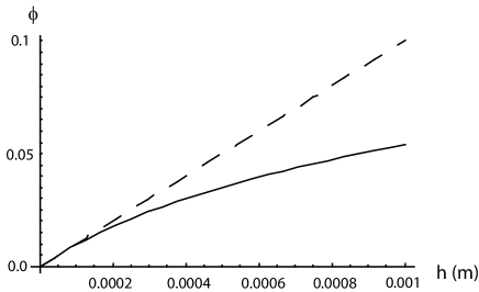
Figure 10: Solution of the retardation condition (solid line) at $\Delta s=0$ as a function of $h$ and comparison with $\phi=\gamma h$ (dashed line)

III.2 Tail-Head interaction

We will now analyze the tail-head part of the interaction when $\Delta s>0$. In the case where the bunch enters the bend we have contributions from retarded sources both in the bend and in the straight line before the bend. The contribution from the retarded sources in the magnet can be obtained by simple integration of Eq. (22), and reads

$${F_{\mathrm{\bot m}}^{\mathrm{B}}}\simeq{e^{2}\lambda_{0}\over{4\pi\varepsilon_{\mathrm{0}}R}}\left[\ln\left({\hat{\phi}_{\mathrm{max}}\over{\hat{\phi}_{\mathrm{min}}}}\right)+{4(2\hat{h}^{2}+\hat{\phi}^{2}_{\mathrm{max}})\over{4\hat{h}^{2}+4\hat{\phi}^{2}_{\mathrm{max}}+\hat{\phi}^{4}_{\mathrm{max}}}}-{4(2\hat{h}^{2}+\hat{\phi}^{2}_{\mathrm{min}})\over{4\hat{h}^{2}+4\hat{\phi}^{2}_{\mathrm{min}}+\hat{\phi}^{4}_{\mathrm{min}}}}\right]~{},$$ (52)

where ”m” is a reminder that the contributions treated by Eq. (52) are all from the ”magnet”. All that is left to do now, is to investigate the values which $\hat{\phi}_{\mathrm{min}}$ and $\hat{\phi}_{\mathrm{max}}$ assume.

Let us first define with $\hat{\eta}$ the normalized angular position of the test particle inside the bending magnet. Now define with $\hat{\phi}^{*}$ the solution of the retardation equation $\Delta\hat{s}_{\mathrm{min}}=\hat{\phi}^{*}/2+\hat{\phi}^{*3}/24-\hat{h}^{2}/(2\hat{\phi}^{*})$. If $\hat{\phi}^{*}<\hat{\eta}$, the retarded position of the first source particle is in the bending magnet, and $\hat{\phi}_{\mathrm{min}}=\hat{\phi}^{*}$. On the other hand, when $\hat{\phi}^{*}>\hat{\phi}$ there are no contributions to the radial force from the bend.

Next, we define with $\hat{\phi}^{**}$ the solution of $\Delta\hat{s}_{\mathrm{max}}=\hat{\phi}^{**}/2+\hat{\phi}^{**3}/24-\hat{h}^{2}/(2\hat{\phi}^{**})$ (in our case $\Delta\hat{s}_{\mathrm{max}}$ will be equal to one half of the normalized bunch length). Supposing $\hat{\phi}^{*}<\hat{\eta}$, if $\hat{\phi}^{**}<\hat{\eta}$ too, then all the particles contribute from the bend, and $\hat{\phi}_{\mathrm{max}}=\hat{\phi}^{**}$. On the other hand, when $\hat{\phi}^{**}>\hat{\eta}$, we have a mixed situation, in which part of the particles contribute from the bend and others from the straight line before the magnet. In this case $\hat{\phi}_{\mathrm{max}}=\hat{\phi}$.

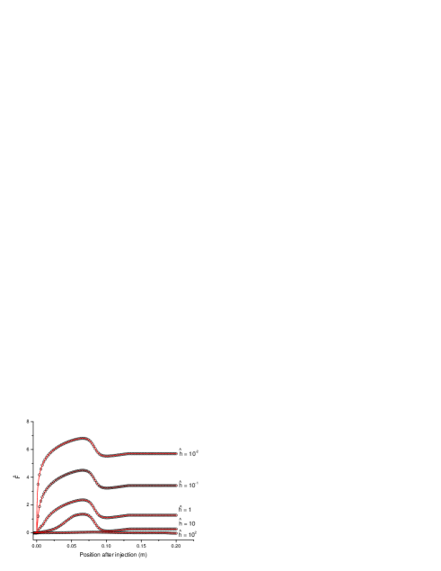
Figure 11: Normalized radial force acting on a test particle from a bunch with rectangular density distribution entering a hard-edge bending magnet as a function of the position of the test particle inside the magnet. The solid lines show analytical results; the circles describe the outcome from $\mathrm{TRAFIC}^{4}$. We chose $\Delta s_{\mathrm{max}}=100\mu$m, $\gamma=100$, $R=1$ m; graphs are plotted for several values of the parameter $\hat{h}$.

Figure 12: Normalized radial force (analytical result) acting on a test particle from a bunch with rectangular density distribution entering a hard-edge bending magnet as a function of the position of the test particle inside the magnet. We chose $\Delta s_{\mathrm{max}}=100\mu$m, $\gamma=100$, $R=1$ m; several curves for different values of $\hat{h}$ are shown. A clear discontinuity in the first derivative is visible.

The contribution from the retarded sources in the straight path before the bend is given by

$${F_{\mathrm{\bot s}}^{\mathrm{B}}}=\int_{\mathrm{\Delta\hat{s}_{\mathrm{min}}}}^{\Delta\hat{s}_{\mathrm{max}}}{R\over{\gamma^{3}}}F_{\mathrm{\bot}}(\hat{y}(\Delta\hat{s},\hat{h}),\hat{\phi})d\Delta\hat{s}~{},$$ (53)

where ”s” stands for ”straight path”, and where the expression for $F_{\mathrm{\bot}}$ in the integrand is given by Eq. (27). It is convenient, as done before, to switch the integration variable from $\Delta\hat{s}$ to $\hat{y}$. The Jacobian of the transformation is given by (see SALLONG )

$${d\Delta\hat{s}\over{d\hat{y}}}\simeq{(\hat{\phi}+\hat{y})^{2}+\hat{\phi}^{4}/4+\hat{h}^{2}\over{2(\hat{\phi}+\hat{y})^{2}}}$$ (54)

After substitution of Eq. (54) and Eq. (27) in Eq. (53), one can easily carry out the integration, thus getting

$${F_{\mathrm{\bot\mathrm{s}}}^{\mathrm{B}}}\simeq{2e^{2}\lambda_{0}\over{4\pi\varepsilon_{\mathrm{0}}R}}\Bigg{[}{\hat{\phi}\left(4\hat{y}_{\mathrm{min}}+2\hat{\phi}+\hat{\phi}^{3}\right)\over{4(\hat{y}_{\mathrm{min}}^{2}+\hat{h}^{2})+8\hat{y}_{\mathrm{min}}\hat{\phi}+4\hat{\phi}^{2}+\hat{\phi}^{4}}}$$

$$-{\hat{\phi}\left(4\hat{y}_{\mathrm{max}}+2\hat{\phi}+\hat{\phi}^{3}\right)\over{(4\hat{y}_{\mathrm{max}}^{2}+\hat{h}^{2})+8\hat{y}_{\mathrm{max}}\hat{\phi}+4\hat{\phi}^{2}+\hat{\phi}^{4}}}\Bigg{]} ~{}.$$ (56)

As done before for $\hat{\phi}_{\mathrm{min}}$ and $\hat{\phi}_{\mathrm{max}}$, we can now investigate the values of $\hat{y}_{\mathrm{min}}$ and $\hat{y}_{\mathrm{max}}$.

Let us start with $\hat{y}_{\mathrm{min}}$. First, we define with $\hat{y}^{*}$ the solution of the retardation condition $\Delta\hat{s}_{\mathrm{min}}=(\hat{\phi}+\hat{y}^{*})/2+(\hat{\phi}^{3}/24)(4\hat{y}^{*}+\hat{\phi})/({\hat{y}^{*}+\hat{\phi}})-\hat{h}^{2}/(2\hat{y}^{*}+2\hat{\phi})$. If $\hat{y}^{*}>0$, the retarded position of the first source particle is in the straight line before the bending magnet, and $\hat{y}_{\mathrm{min}}=\hat{y}^{*}$. On the other hand, when $\hat{y}^{*}<0$, the retarded position of the first source particle is in the bend, and $\hat{y}_{\mathrm{min}}=0$.

Next, we define with $\hat{y}^{**}$ the solution of $\Delta\hat{s}_{\mathrm{max}}=(\hat{\phi}+\hat{y}^{**})/2+(\hat{\phi}^{3}/24)(4\hat{y}^{**}+\hat{\phi})/({\hat{y}^{**}+\hat{\phi}}-\hat{h}^{2}/(2\hat{y}^{**}+2\hat{\phi}))$ (again, in our case $\Delta\hat{s}_{max}$ is just half the bunch length normalized to $R/\gamma^{3}$). Consider the case $\hat{y}^{**}<0$: all the particles contribute from the bend, that is we entered the steady-state situation. In this case $\hat{y}_{\mathrm{max}}=\hat{y}_{\mathrm{min}}=0$. On the other hand, when $\hat{y}^{**}>0$, we have again a mixed situation, in which part of the particles contribute from the bend and others from the straight line before the magnet. In this case $\hat{y}_{\mathrm{max}}=\hat{y}^{**}$.

The following step is to actually plot the radial force exerted on an electron by a bunch with rectangular distribution entering a long bend. Our results, compared, once again, with simulations by $\mathrm{TRAFIC}^{4}$, are shown in Fig. 11 for a bunch length of $100~{}\mu$m, $\gamma=100$, $R=1$ m and for different values of $\Delta\hat{s}$. A perfect agreement is obtained with the results by $TraFiC^{4}$. A first characteristic length is obviously given by the solution of the retardation condition with $\Delta s=l_{b}/2$, and gives the position at which the test particle begins to feel a steady interaction from the tail sources. There is a second characteristic length more difficult to see, though: a careful inspection of Fig. 11 shows, in fact, a small irregularity (actually a discontinuity in the first derivative) in the curve for $\hat{h}=1$ at the position $z\simeq 1~{}cm$. Such irregularities are present in all the curves in Fig. 11, although one has to look carefully for them by magnifying parts of the plots, as shown in Figs. 12A-D. It is this fact which actually suggests the presence of a second formation length.

When the value of $h$ is small the discontinuity is located, approximately, at $z\simeq\gamma h$: for example when $h=1~{}\mu m$, in Fig. 12A, we have a discontinuity in the first derivative of the curve at $z\simeq 0.1~{}mm$. Nevertheless, this value changes as we increase h. In fact, when $h=1~{}mm$, in Fig. 12C, the discontinuity is at $z\simeq 5.4~{}cm$, while when $h=1~{}cm$, in Fig. 12D, we find a value of $z\simeq 18.6~{}cm$: these are the same numerical values found when discussing the entrance in the steady state of the Head-Tail interaction in the previous subsection. The reader will remember that these are, in fact, the solutions of Eq. (51). From a physical viewpoint, the solution of Eq. (51) is the position at which the test particle begins to feel the electromagnetic signal from the source at $\Delta s=0$.

Before that point, the test particle feels interaction from particles behind it but only due to velocity fields, since the retarded positions of all the electrons behind the test one are not yet in the bend. After that particular point, the force on our test electrons has a component due to the acceleration field too. This suggests that the physical meaning of the presence of this second formation length is simply the switching on of the contribution of the acceleration field. As a last remark it is interesting to note that Tail-Head and Head-Tail interactions have a characteristic length in common, but for completely different reasons.

IV SUMMARY AND CONCLUSIONS

In this paper we presented a fully electrodynamical study of transverse self-forces within an electron bunch moving in an arc of a circle in the case the test particle is endowed with a vertical displacement $h$. We strived for a generalization of the results obtained in OURS in order to obtain a better qualitative and quantitative explanation of the physics involved in the problem and, in particular, to explain the behavior of the self-interaction depicted in Fig. 1.

First we generalized the results in OURS in the case of a two-particle system. Then, by integration of these results, the case of a line bunch and a test particle with a vertical displacement was studied. This case includes all the relevant physics present in the situation of a bunch with vertical size.

Besides allowing one to generalize results obtained in OURS , our study aimed at a physical understanding of the results by $TraFiC^{4}$: we found that the bunch can be divided into four separate regions (over which one can integrate the two-particle interaction) corresponding to four different types of source-test interaction, namely head-tail with $|\Delta s|<h$, head-tail with $|\Delta s|>h$, tail-head with contributions from velocity fields alone, and tail-head with contributions from both acceleration and velocity field. We found that these regions correspond to four characteristic formation lengths, which can be determined quantitatively by simple analytical calculations.

For the first, the third, and the fourth region, we could use relatively simple analytical results in order to describe the situation and easily perform crosschecking with $TraFiC^{4}$. The perfect agreement we found gives us much information: this constitutes, in fact, a reliable cross-check which provides, at the same time, very strong indication that the code calculates the self-interaction in the proper way and that the approximations which we made in our analytical theory are correct. Moreover, we have physical explanations of the self-interactions in terms of formation-lengths and type of source-test interaction.

Because of mathematical difficulties linked with the structure of the retardation condition we left the quantitative discussion of the second region ($-h<\Delta s<0$) for future work. Nevertheless we were able to understand the physical meaning of this region and to determine its formation length.

V ACKNOWLEDGEMENTS

The authors wish to thank Reinhard Brinkmann, Yaroslav Derbenev, Klaus Floettmann, Vladimir Goloviznin, Georg Hoffstaetter, Rui Li, Torsten Limberg, Jom Luiten, Helmut Mais, Philippe Piot, Joerg Rossbach, Theo Schep and Frank Stulle for their interest in this work.

References

- (1) G. Geloni, J. Botman, J. Luiten, M. van der Wiel, M. Dohlus, E. Saldin, E. Schneidmiller and M. Yurkov, DESY 02-048, submitted to Phys. Rev. E
- (2) TESLA Technical Design Report, DESY 2001-011, edited by F. Richard et al. and http://tesla.desy.de/
- (3) W. Knulst, J. Luiten, M. van der Wiel and J. Verhoeven, Applied Physics Letters 79, 2999 (2001)
- (4) K. Rothemund, M. Dohlus and U. van Rienen, in Proceedings of the 21st International Free Electron Laser Conference and 6th FEL Applications Workshop, Hamburg, 1999, edited by J. Feldhaus and H. Weise
- (5) TESLA Technical Design Report, DESY 2001-011, edited by F. Richard et al., and http://tesla.desy.de
- (6) Ya. S. Derbenev, J. Rossbach, E. L. Saldin and V. D. Shiltsev, TESLA-FEL Report No. 95-05, DESY, Hamburg, 1995
- (7) E. L. Saldin, E. A. Schneidmiller and M. V. Yurkov, Nucl. Instr. Methods A 398, 373 (1997)
- (8) R. Li, C. L. Bohn and J. J. Bisognano, in Proceedings of the SPIE Conference, San Diego, 1997, vol. 3154, p. 223
- (9) G. Geloni and E. Saldin, DESY 02-201, submitted to Am. Journ. of Physics
- (10) E. L. Saldin, E. A. Schneidmiller and M. V. Yurkov, Nucl. Instr. Methods A 417, 158 (1998)
- (11) R. Li, in Proceedings of the 2nd ICFA Advanced Accelerator Workshop on The Physics of High Brightness Beams, Los Angeles, 1999.
- (12) G. Geloni, V. Goloviznin, J. Botman and M. van der Wiel, Phys. Rev. E 64, 046504
- (13) M. Borland, Phys. Rev. Special Topics 4, 070701 (2001)
- (14) R. Talman, Phys. Rev. Letters, (1986)
- (15) E. P. Lee, Partcle Accelerators , (1990)
- (16) Y. Derbenev and V. Shiltsev, in Fermilab-TM-1974 (1996)
- (17) G. Stupakov, in Proceedings of the ICFA conferfence Arcidosso, 1998
- (18) G. Geloni, E. Saldin, E. Schneidmiller and M. Yurkov, DESY 03-31