Internet websites statistics expressed in the framework of the Ursell-Mayer cluster formalism
D. Bara
aDepartment of Physics, Bar Ilan University, Ramat Gan, Israel
We show that it is possible to generalize the Ursell-Mayer cluster formalism so that it may cover also the statistics of Internet websites. Our starting point is the introduction of an extra variable that is assumed to take account, as will be explained, of the nature of the Internet statistics. We then show, following the arguments in Mayer, that one may obtain a phase transition-like phenomena.
Keywords: Internet, Ursell-Mayer formalism, Phase transition, Combinatorics
1 INTRODUCTION
The use of the Internet as a necessary tool for easing the application of an increasing number of diverse tasks, and not only for web surfing, is fastly growing. There has been lately an ongoing research that discusses the Internet topology [1, 2] where use is made of the fractal [3, 4] and the percolation theories [5, 6, 7]. In these works the Internet is regarded as random network [4, 5] and the websites as its building blocks.
We focus our attention here on the unique nature of the websites which enables the possible existence in them of any number of links that refer to other sites that may be downloaded by a single click of the computer mouse. As known, any fractal is built by repeated iteration (see Aharony in [5]) of some unique natural "microscopic" growth rule which is rather special in the Internet case. This is because not only the forms of the constituent websites, the identity and connectivity [4, 5, 6] of their links depend only on the programmers that write the relevant softwares but also the growth of the web itself depends exclusively upon them. Thus, for taking into account the nature of programming that enables one to display on the computer screen practically anything we introduce a special variable, denoted in the following by , that corresponds to the spatial variable which is used to discuss the statistics of the particle system. The character of this variable will be discussed in the following section.
We note that similar situations arise in the discussion of some mathematical [8] and physical [9] situations for which one have to add a special variable that takes account of some nonphysical properties of the discussed systems. For example, in the functional generalization [10] of Quantum Mechanics the generalized Hilbert space (the Lax-Phillips one [9]) is obtained by adding an extra variable to the conventional Hilbert space. A similar addition of an extra variable has been proposed by Parisi-Wu-Namiki [11, 12] in their stochastic Quantization theory which assumes that some stochatic process [13] occurs in the extra dimension.
As known, any web site contains one or more web pages and each of these may include one or more links to other places on the same page or to other sites or other web servers. The user that clicks, through the keyboard, on any link (the highlighted addresses (URL)) downloads its relevant site to the screen. The number of the links in a web site may be small (or even zero for the unlinked web sites) or it may be very large. We do not consider here the secondary links that may be found on the sites referred to by the first links.
We discuss the connectivity [1, 2, 4, 5] among the Internet websites where by this term we mean the amount and degree of the interconnection among the sites that compose the Internet network. Thus, a large connection among the sites of the Internet denotes a corresponding large connectivity and vice versa. Our aim in this work is to show that if we consider large clusters of mutually linked sites then adding even a very small amount of connecting links results in a disproportionally large growth of the total connectivity [4, 5] of these clusters. We use, for that purpose, a generalized version of Ursell [14] and Mayer [15, 16] cluster formalism. This generalization is obtained by the introduction of the remarked extra variable that takes account of the unique Internet statistics. We note that similar discussion in Ursell [14] and Mayer [15] with regard to the large clusters of particles results in demonstrating phase-transition phenomena [14, 15, 16].
In Section 2 we discuss the Internet using the partition function method [15, 16, 17] where the relevant "configuration integral" is discussed by generalizing the cluster formalism of Ursell [14] and Mayer [15]. This generalization is imposed by the unique nature of the Internet websites which allows, as will be shown, more than one kind of linkage between the sites. Thus, the typical numbering procedure and the combinatorics of the Ursell-Mayer method, which was originally formulated for discussing the -particle system, has to be appropriately expanded. In Section 3 we discuss and generalize the relevant statistical integrals and in Section 4 we show the mentioned phase transition of the connectivity among the Internet websites. Note that our discussion in this work is general in that we do not specify the nature and identity of the relevant sites.
2 THE ADAPTATION OF THE URSELL-MAYER CLUSTER FORMALISM FOR THE INTERNET WEBSITES
2.1 The definitions of the "position", the "distance" and the "potential" between websites
We show in this work that the connectivity [4, 5] in large -site clusters, which is determined by the links in all the sites, is so sensitive to these connecting links that adding even a small number of them to the cluster results in a giant increase of its overall connectivity. This large growth of the connectivity, compared to the small addition of links that causes it, constitutes a phase transition which should be discussed in the appropriate terms and terminology. For that purpose we adapt a generalized version of the virial expansion of the equation of state [16, 17] which is discussed by using the cluster formalism developed by Ursell [14] and Mayer [15]. We assume that the web sites system discussed here is composed of sites where is generally a large number. We note that when one discuss the potential energy of the particle system in the configuration space [16, 17] the relevant variable is the distance between any two particles and which depends only on their positions. Thus, the potential between them is assumed to be effective for small ranges of and vanishes when grows.
Here, also for the site system we denote by the "potential" between the two sites and which depends upon the "distance", denoted here by , between them. This “distance” signifies how much these sites differ from each other so that it is shorter the more “similar” they are and longer for unrelated sites. The distance between and may be assigned a Quantitative aspect by taking into account the number of common links to both so that the larger this number is the shorter this distance becomes. That is, each site is characterized by all its links so that its "position" in space may be written as , where, , , etc denote the links in to the sites 1, 2, 3, etc. Thus, as the real positions in configuration space are measured relative to the origin (zero values for coordinates) so the "positions" of the sites here are "measured" relative to the unlinked site which has zero link. That is, the more linked some site is the larger is its "distance" from the "origin" (the unlinked site). In this context we may use Figure 1 in order to make this point clearer. Thus, the unlinked sites denoted [7] and [8] at the right hand side of the planar diagram of Figure 1 are at the largest "distance" from each other and from the other sites of the figure. On the other hand, the doubly linked sites [15], [16], [23] and [24] in this figure have a very small "distance"
from each other. In such a manner one may write the "distance" between and , for example, as . Thus, we may define a "potential" , in analogy to the particle system, for example, as
| (1) |
The potential between the sites and does not have a physical meaning but only a statistical one. This is because it depends upon the distance between these sites which is, as remarked, determined not only by their mutual links (to each other) but also by all the other shared and common links which may be very large in number. Thus, this potential have a statistical meaning (see the discussion after Eq (6) and (7) and the Appendix) which is expressed using Combinatorical analysis.
The potential from the last equation, as for the corresponding , is effective for small “distances” and vanishes when grows. However, in contrast to the particle system in which the distance between any two members and is sharply and uniquely determined by their positions only here the "distance" between any two sites is also characterized, as has been remarked, by other links to other sites that are common to both, besides the links that refer to each other. Moreover, since, as remarked, the linking among the sites are effected through the highlighted places (upon which one press with the mouse pointer to download the linked site to the screen) a site may have such a link to another one whereas the second have no link to the first. Thus, in order to discuss appropriately the potential between any two sites and one must differentiate between four different situations; (1): has a link to and has no one to . (2): has a link to and has no one to . (3): both and have no links to each other. (4): both and have links to each other in which case the connectivity between them is larger than in cases 1 and 2.
2.2 The "Thermodynamical" discussion and representation of the Internet
The mentioned possible different kinds of linkings between the sites influences the standard expressions and formulas of the Ursell-Mayer expansion [15] in such a manner that the application of it to the Internet statistics becomes, as will be shown, delicate and complicated. First, we note that the use of physical thermodynamical methods for discussing the Internet structure enables one not only to use the variable in an analogous manner to the spatial variable but also to use other thermodynamical quantities. We note in this context that the use of Thermodynamics terminology and terms for discussing other (nonphysical) branches of science may be found in the general literature (see, for example, [18, 19]). Thus, we may discuss an appropriately defined partition function as well as the related "pressure" and the "free energy" in the linked cluster of websites. We show by applying these fundamental concepts to the Internet that the remarked phase transition of the cluster’s connectivity may be related to the internetic "pressure" of its sites. This will be demonstrated for large clusters of sites which are doubly connected to each other as in (4) above (see the discussion after Eq (1)) in which case adding even a small number of links results in a disproportional enormous strengthening of the overall connectivity. We first define the appropriate "partition function" that determines the states of the site ensemble and the correlation among them
| (2) |
As seen, we use the same expression for as used in [16, 17] except for the dependence upon the variable . The is generally an exponential function that does not depend upon the potential and is the “configuration integral” in space which is given here by the same form, except for the dependence, as that of the particle system [16, 15]
| (3) |
The variable denotes that we discuss Internet sites and each of the differentials signifies an infinitesimal "volume" element in -space. Thus, if we assume, analogously to the configuration space, that this space may be projected into three axes denoted by , and then the differential in Eq (3) may be written as . Now, since denotes, as remarked, the “distance” between the sites and (see discussion before Eq (1)) then we may regard the integrals in Eq (3) as ranged over all "distances" from a reference site which corresponds to the origin of the configuration space. This reference site is, as remarked before Eq (1), the unlinked site (with zero links). The in the exponent has dimension of "inverse energy" and corresponds to the of the particle ensemble [15, 16, 17]. Thus, from Eqs (2)-(3), and analogously to the particle system [15], one may define the appropriate "pressure" and "free energy" as
| (4) |
| (5) |
Note that the forms of and are the same, except for the dependence, as those of the particle system [15]. The boldfaced and in Eqs (4)-(5) denote respectively the volumes in space available for and one sites and the in Eq (5) is the work function in this space which corresponds in its expression to the analogous work function or the Helmholtz free energy of the particle system [15, 16, 17]. In order to be able to use and interpret the Quantity (and ), and especially to show that it is related to the mentioned phase transition, we have first to express from Eqs (2)-(5) in a form appropriate for discussing Internet websites. This form is found if we first ascertain the proper numbering procedure suitable for the linked sites and which is taken care of by the potential . Thus, we write this as a sum of terms each of which depends on the “distance” between any two sites and which denotes, as remarked, the connectivity between them. Now, since each two sites may be connected to each other in three different ways as in the situations labelled , , and in the discussion after Eq (1) we get the result that in a system of sites there are different pairs so that the potential is
| (6) |
The first double sum takes account of the pairs that are singly connected to each other and the second covers the that are doubly connected and is the potential of the pair of sites and as a function of the “distance” between them (see Eq (1)). Note that the number of doubly connected pairs is half that of the singly connected ones since a single connection between any two sites and may be realized in two different ways (see the situations , and in the former discussion) compared to the double connection between them which is realized in only one way. We define, as done when discussing the cluster function theory [14, 15, 16], the function
| (7) |
We see that for a large “distance” (unrelated web sites) where tends to zero (see Eq (1)). Note that when the sites and have no links to each other (unrelated sites) then they, naturally, also have no other common links so that and are both zero. Also, as one may realize the probability to find two sites that are entirely identical to each other is very small so that in this case becomes very large (see Eq (1)) such that . By we denote the one-way connection from site to site when there is a link in to , and the double connection between them is denoted by where, obviously, we have (see Eqs (1) and (7)) . The “configuration integral” from Eq (3) becomes using the last equations
| (8) |
Note that due to the special character of the websites, as discussed after Eq (1), the counting relation between the general sites and is as written in the subscripts of the summation signs of the last equation (compare with the analogous expression in the particle system (see Eq (13.3) in p. 277 in [15])).
2.3 The plane diagrammatic structure of the linkings among the websites
Now, in order to be able to cope with the terms under the parentheses signs in Eq (8) we use an extended version of the one to one correspondence [15, 16] made between the terms of of the -particle ensemble and certain planar diagrams. For example, the diagram shown in Figure 1 for corresponds to the term in Eq (8) that involves , , , , , , , , , , , , , and (we have inserted commas between the and components of ). As seen from the diagram the sites (denoted in this paragraph by curly brackets) are assembled in clusters, so that the sites {7}, {8}, {14}, and {22} each constitutes a single cluster of 1 member. The sites {1}{2}, {5}{6}, and {17}{18} are in clusters of two where the pairs {1}{2} and {17}{18} are doubly connected. The sites {3}{4}{9}{10} and {15}{16}{23}{24} are clusters of 4 where the members of the first are singly connected to each other whereas those of the second are doubly connected. The sites {11}{12}{13}{19}{20}{21} constitute a six-member cluster. As seen from Figure 1 the sites in a cluster are connected in a different manner to each other so that one may be doubly connected to all the other sites of the cluster in which case its connectivity is maximal whereas another may be singly connected to only one site so that its connectivity is minimal. For example, in the six member cluster of Figure 1 the site {20} is doubly connected to the sites {11}, {12}, and {19} and singly connected to {13} and {21}, whereas the sites {13} and {21} are each singly connected to only the site {20}. This difference between the connected sites and the less connected ones is realized when one remove from the cluster one site and all its connecting lines. Thus, if the removed site is the densely connected one the connectivity of the remained cluster is weakened considerably whereas if the removed site is slightly connected the effect on the connectivity of the remaining cluster is less influential. For example, if the site {20} and all its connecting lines in the six-member cluster of Figure 1 is removed the cluster is actually broken into three different smaller ones whereas if either the site {13} (or {21}) is removed together with its single connecting line the connectivity of the remaining 5-member cluster is only slightly affected.
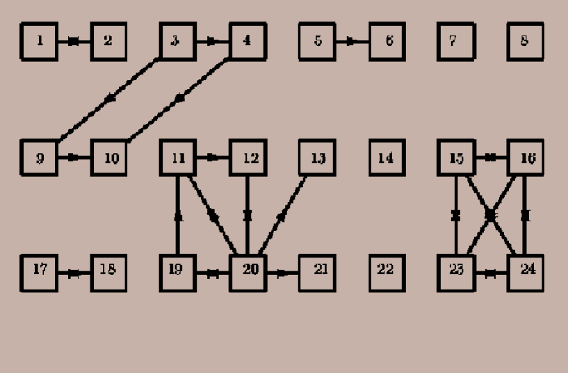
We note that Figure 1 is reminiscent of Fig 13.1 in page 278 in [15] which shows a similar diagram for 28 molecules. The principal difference between the two diagrams is that in Figure 13.1 in [15] the connection, if exists, between any two molecules is unique and not directed as in the plane diagram of Figure 1 here. That is, as remarked, the linking between any two sites may be of three kinds and the lines that connect them reflect this diversity of connection.
2.4 The ordering of the sums of the integrals of into clusters
We denote the number of times an -site cluster appears in a term by so that the total number of all the sites may be written, as for the analogous particle system [15], as . Note that the integrals over the sites in different clusters of one term in Eq (8) are independent of each other. Thus, the integral of a term in Eq (8) is the product of the integrals over the sites in the same cluster where the meaning of the integral over the variable is as discussed after Eq (3). As for the particle system [15] we sum the integrals of all the products that occur when a specified -sites are in one cluster and, because of the different counting of Internet websites, we divide this sum, denoted by , into two different parts as
| (9) |
where , denote the products over the mixed and doubly connected sites respectively. By the term mixed we mean that the sites in the relevant cluster may be either only singly connected or both singly connected (to some sites) and doubly (to others, see the example of in Eq (10)). Note the different counting relations between the general sites and for the mixed and doubly connected sites as expressed respectively in the subscripts of the two product signs of Eq (9). The counting relation of for the doubly connected sites, which is the same as in the analogous particle system (see p. 277 in [15]), is because this kind of connection is unique and does not depend on direction. The number of in each term of the ranges from a minimum of to a maximum of and the corresponding number in the part ranges from a minimum of to a maximum of where these numbers are always even for . The product is a normalization factor where is, as remarked, the total volume in -space of all the sites. For example, is
| (10) | |||
The is given by the first four terms and is given by the rest. Note that since each mixed connection between any two sites may be, as remarked, of three kinds there are 50 terms in whereas only 4 terms in because the double connection is unique. We thus see that becomes very large for increasing values of as may be realized from Appendix A in which we use combinatorical analysis for calculating the number of terms in for general .
3 THE "CONFIGURATION INTEGRAL" , THE CLUSTER INTEGRALS AND THE IRREDUCIBLE INTEGRALS
3.1 The expression of in terms of
From the discussion of the former section we realize that the total contribution to the “configuration integral” from each specific -cluster is [15]
| (11) |
which is the expression obtained also for the particle system (see p. 280 in [15]) except that here we use the volume in space. The product has been introduced to cancel the effect of the normalization constant (see Eq (9) and the discussion following it) and is, as noted, the number of times an -cluster appears in a term. Now, we add all the similar contributions from the other -site clusters which is obtained by mutiplying the expression from the last equation by which is the number of ways to distribute different sites into clusters so that clusters have one site each, clusters have two sites each … and clusters have sites each. The division by (and not by as for the particle system (see page 281 in [15])) is because of the unique nature of the websites which are not only different from each other but also render their clusters, even those with the same number of sites, different. That is, the division takes into account the permutations of the sites inside the clusters and also the permutations of the clusters that have identical number of sites. The overall contribution from all the site clusters is therefore
| (12) |
The last step is to sum over all values of so that we obtain for the total value of the “configuration integral” divided by
| (13) |
where we have used the relation which is the volume in space per site. As seen from the last equation the indices and over which the sum and the product are respectively run must satisfy the condition [15] (see the discussion before Eq (9)).
3.2 The ordering of the cluster integrals into irreducible integrals
As realized from the last equations, there are many terms in which represent clusters that are composed of two parts that are connected by only one link, so that removing it splits the relevant integral into a product of two. Thus, the cluster integrals ’s may be simplified as in the particle system [15, 16] by representing them as sums of integrals that can not be further reduced into a product of integrals. That is, these irreducible integrals, denoted as , correspond to clusters all the members of which are more than singly connected as follows
| (14) |
where, the product is over all the sites each of which is connected to at least two other sites. Note that since, as remarked, the connection between any two sites and may be of more than one kind (see the discussion after Eq (1)) the counting relation is as written in the subscript of the product sign (and not which is appropriate for the particle system (see p. 287 in [15])). As for the from Eq (9) we differentiate between and which denote mixedly and doubly connected sites respectively where by the term mixedly we mean that the sites in the relevant cluster may be, as for the , either only singly connected or both singly connected (to some sites) and doubly (to others). From Eqs (7), (9) and (14) we see that the terms of and may be positive or negative depending upon the evenness or oddness respectively of the numbers of in these terms. The terms of and , on the other hand, are always positive since the number of their is always even.
The first two , for example, are
| (15) | |||
The coefficients of 2, 6, and 12 signify the number of similar terms that differ only by the direction of the connecting lines between the sites. Thus, the term denotes the six possible different ways to construct a 3-cluster from three singly connected sites since each of these sites may be connected in two different ways to its neighbour. Likewise, the term denotes the 12 different possible ways to construct a 3-cluster from two doubly connected sites which are singly connected to the third. This is because there are 3 different ways to select the two doubly connected sites from three and for each of these there are four different ways to singly connect these two sites to the third one. Now, we can write, analogously to the particle system [15], any cluster integral as a sum of terms each of which depends upon the powers of the integrals where and are related by . The in the last relation is because one site is left over due to the definition of (see the discussion before Eq (14)). Thus, using the arguments in the Appendix in [15] (see p. 455-459 there) with respect to the particle system we write the following dependence of upon
| (16) |
where we take into account that the number of ways to distribute different objects into clusters of objects each (with ) is . The expression (16) results also from considering the three possible connections between any two sites that introduce different counting (see the discussion before Eq (12) and after (15) and note the similarity between Eqs (13) and (16)).
3.3 The general term of as a function of and that of as a function of
We follow in this subsection the same steps and the same expressions, used by Mayer [15] in his demonstration of phase transition for the particle system, except for the variable and the mentioned generalization necessary for discussing the Internet websites. That is, we demonstrate, using the following equations (17)-(23), that the overall connectivity of the doubly linked cluster may undergoes phase-transition.
We begin by using the Stirling approximation [20] for , , and so one may write the logarithms of the general terms of the sums of Eqs (13) and (16), denoted by and respectively as (compare with Eqs (13.13) and (14.2) in [15])
| (17) | |||
Now, if all the ’s are positive one may replace [15], for large values of , the logarithm of the sums in Eqs (13) and (16) by that of their largest terms. These are obtained from Eqs (17) by subtracting from the first of which the constant multiplied by the condition and from the second the constant multiplied by the condition . These kinds of operation and the denotation of the constants as and are done, as in [15], for a clear representation of the relevant calculations.
We, now, differentiate the first of the resulting expressions (related to ) with respect to and the second (related to ) with respect to and equate to zero so that the values of and that maximize and respectively are
| (18) |
Note that, due to the nature of and (see Eqs (9) and (14)), both and have dimension of inverse . Substituting for in the second of Eqs (17) and regarding the resulting expression, in the limit of very large , as representing the logarithm of the sum in (16) one obtains, neglecting the terms and compared to and using the condition for large (instead of )
| (19) |
where , which leads to
| (20) |
Compare with the analogous expressions (14.6)-(14.7) in [15] for the particle system. From the last two equations one obtains, in analogy to the particle system [15]
| (21) |
where is small compared to so that it satisfies . Now, the condition may be written, using the first of Eq (18), as
| (22) |
Substituting for from Eq (21) into the last equation, dividing by , and using for large the approximation one obtains
| (23) |
The last equation, as shown in the next section, is central in demonstrating that enlarging the remarked connectivity even slightly, by adding the same links to them, results in an enormous strengthening of the overall connectivity.
4 THE PHASE TRANSITIONAL STRENGTHENING OF THE CONNECTIVITY AMONG THE INTERNET WEBSITES
4.1 The results for a cluster of sites
We, now, assume that the number of sites of the -cluster is large and that they are doubly connected to each other, in which case both and are, as remarked, positive due to the even number of their . Thus, dividing both sides of Eq (23) by and taking the logarithm of the term that corresponds to we obtain for this term (denoted )
| (24) |
The expression may be written as so that if then , and when is negative is smaller than unity and the relevant term in Eq (24) is negative. In this case since it is the dominant term on the left hand side of Eq (24) is also negative, which implies that is smaller than unity and its contribution to the sum in Eq (23) is small. Thus, for exemplifying the remarked giant increase of the connectivity we assign to the value of and take into account the former result of , which requires to be much smaller than . So, if increases from zero by only the small amount of , due to adding a small Quantity of linked sites to the cluster, the value of grows, as a result of this, by and the contribution of to the sum increases by . That is, adding even a small number of connecting links to a large cluster of connected sites results in a disproportional strengthening of the connectivity of this specific cluster.
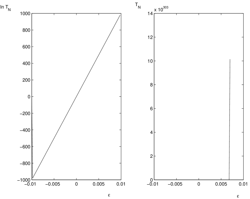
The previous results may be realized from the two Subfigures of Figure 2 which show and from Eq (24) as functions of in the range and for . The left hand side Subfigure shows the change of from Eq (24) in the neighbourhood of where we have written and ignore the term which vanishes for large . Thus, one may see that is proportional to where the coefficient of proportion is . But the behaviour of (compared to that of ) is not the same for positive and negative as may be seen from the right hand side Subfigure of Figure 2. That is, although negative may produce large negative values of as seen in the left hand side subfigure it yields a rather negligible change of . But when departs slightly from zero towards positive values the produced change in becomes so enormous that even the small change of , yields the giant change of . That is, the overall connectivity of the large cluster has undergones, as remarked, a phase transition change.
4.2 The inverse proportionality between the connectivity in a large cluster and the "volume" per site in space
Now, remembering that Eq (24) was obtained after dividing both sides of Eq (23) by we have to conclude, in order to retain Eq (23), that must decrease in this case to a correspondingly very small value where, as noted, is the "volume" in space per site. For a better understanding of the meaning of a small we return to Eq (4) for the "pressure" and evaluate it in the limit of large . In such case one may replace, as remarked, , where is given by Eq (13), by from the first of Eqs (17). Thus, using and (see the first of Eqs (18) and Eq (13)) we may evaluate the "pressure" from Eq (4) as follows
| (25) | |||
Substituting the last result in the expression for the "free energy" from Eq (5) we obtain . Note that although contains the total "volume" in its denominator (see Eq (9)) it certainly does not depend on it since the integrals of always lead to a factor that cancels that in the denominator. Thus, from the last equations we see that the "pressure" (and the "free energy" ) becomes very large for very small . The meaning of small may now be understood by recalling that the sites of the relevant linked cluster are related to each other by the variable that denotes the “distance” between them in the sense of how much they are similar to each other (see the discussion before Eq (1)). That is, small for the large cluster of doubly linked sites means that the "distances" that signify the differences between them become also very small and they all turn out to be similar to each other. The vanishing "distances" between the sites in this case results in high values for the "pressure" and the "free energy" (see the last equations) of these "jammed" sites. This occurs, as remarked, when adding a small amount of links to the larger terms of the sum in Eq (23) which results in the outcome that the overall connectivity among the component sites becomes maximal in the sense that they have the same links and so they are similar to each other.
Note that the former discussion depends on the assumption that all the are positive whereas we know that the signs of and alternate due to the evennes and oddness of the number of (see the discussion after Eq (14)). But if we confine our discussion to only the doubly connected sites then all the and are, as remarked, positive (in addition to their being mutually connected as required) so all the former discussion is obviously valid. That is, the doubly connected clusters may show this kind of phase transition-like of the connectivity by only adding a very small amount of connecting links. Note that the mathematical expressions of the doubly connected site system are the same as the particle system discussed in [15] except that in the websites system all the and are positive whereas they alternate in sign for the particle system. Also, this kind of avalanche (or condensation as termed in [15]) have been shown in [15] for the particle system provided one assumes that all the are positive (as here).
We note that the process just described of a large increase in the fraction of the connectivity in linked large-size clusters is frequently encountered in ensembles of shared computers connected to each other and to the Internet. In this case an additional web site in the form of a file that has been programmed intentionally for the purpose of adding and connecting it to the other files of the shared ensemble enhances the connectivity of these members to a very high degree. For example, suppose that all these members use some utility program and that not all of them have the same version of it but use several ones. Thus, adding an updation file of this program to them turns all the different versions into one that is common to all thereby increasing very much the total connectivity of them.
5 CONCLUDING REMARKS
We have discussed the Internet statistics using a generalized version of the Ursell-Mayer cluster formalism [14, 15, 16]. We discuss the relevant elements of the Internet, which are the websites, by introducing a new variable that takes account of the unique nature of them. The special character of the Internet, unlike any other common fractal web, is especially demonstrated through the links in its websites which may be of several kinds as discussed after Eq (1). Taking into account this unique character and introducing the relevant expressions into the Ursell-Mayer framework we have shown that one may obtain a phase-transition phenomena. This occurs when a large cluster of doubly linked sites are added an extra small amount of connecting links in which case the contribution of this cluster to the overall connectivity of the entire ensemble becomes enormous. These phase transition changes were also seen to characterize the "pressure" and the "free energy" .
6 ACKNOWLEDGEMENT
I wish to thank L. P. Horwitz for discussion on this subject and for reading the manuscript.
Appendix A APPENDIX: THE COMBINATORICS OF THE -SITE CLUSTER
We calculate in this Appendix the number of terms contributed to the “configuration integral” by any specific . This contribution is valid only when the sites in the same cluster are linked to each other and is obtained by exploiting the special character of the from Eq (9) in order to find all the possible ways by which it contributes to the configuration integral. We take into account that the number of in the terms of ranges, as noted, from to and that each denotes, as remarked, a link to site in site . Thus, the contribution of each may be obtained by calculating the number of possible ways by which each of the Quantities of links , may link sites among them so as to construct an -site cluster. We begin from the least linked -cluster which is constructed by using only different links. The number of ways to construct such cluster is (we denote this number )
in the middle expression is the number of combinations required to construct this least -site cluster where there are no two links in any of these combinations that refer to each other such as and . Now, since, as remarked, the number of in the terms of Eq (9) ranges from to we have, in order to find all the possible different contributions of each , to calculate also the . Each of these is found by first constructing the minimally connected -cluster from sites as in Eq (A.1) and since each site in the -cluster may be linked to all the other sites, except to itself, the next step is to link each of the sites to all the others. That is, the total number of ways to compose an cluster using a number of links that ranges from to is . in the former sum is given by Eq (A.1) and each one of the other ’s is obtained by noting that after composing the minimally linked -cluster using the links, from the possible , one remains with links. These links, in contrast to the former least linked cluster, may be formed so that it is allowed to count also mutually linked sites such as and . That is, for calculating the number of ways to link these additional links we may permute them instead of the former combinations used for the initial links. Thus, as remarked, for calculating we first construct the least linked cluster, using links as in Eq (A.1), and then we link the remaining links which range from 1 for to for . For example, the number of possible ways to construct an site cluster using links, where is given by the recursive relation
The factor in the middle expression is the number of ways to link the remaining links, from the initial possible , after linking links. When we obtain from Eq (A.2) . From the last equation one obtains the number of ways for using links, from a total of , to construct an cluster where the first links are used to initially compose the least linked cluster and the additional link may be anyone from the remaining . When one obtains from Eq (A.2) . Now, we can calculate the sum in order to find the number of ways by which one may build an -site cluster. That is, we write, using the former equations
The last result is the number of terms of and it is very large for large .
References
- [1] M. Faloutsos, P. Faloutsos and C. Faloutsos, "On power-law relationships of the Internet topology", Comput. Commun. Rev. 29, 251 (1999).
- [2] R. Albert and A. -L. Barabasi, "Statistical Mechanics of complex network", Rev. Mod. Phys, 74, 47 (2002); R. Albert, H. Jeong and A. -L. Barabasi, "Error and attack tolerance of complex networks", Nature, 406, 378-382 (2000).
- [3] Benoit. B. Mendelbrot, The Fractal Geometry of Nature (Freeman, New York, 1983).
- [4] A. Bunde and S. Havlin, eds. Fractals in Science (Springer, 1994).
- [5] A. Bunde and S. Havlin, eds. Fractals and Diordered Systems (Springer, New York, 1996).
- [6] D. Stauffer and A. Aharony, Introduction to Percolation Theory (Taylor Francis, London, 1991).
- [7] M. Newman, "The structure and function of complex networks", SIAM Review, 45, 167-257 (2003).
- [8] I. M. Gelfand and N. Ya. Vilenkin, Generalized Functions, Vol 4 (Academic, New York, 1964); Michael Reed and Barry Simon, Methods of Modern Mathematical Physics: Functional Analysis (Academic, London, 1980).
- [9] P. D. Lax and R. S. Phillips, Scattering Theory (Academic, New York, 1967).
- [10] L. P. Horwitz and C. Piron, "The unstable system and irreversible motion in Quantum Theory", Helv. Phys. Acta, 66, 693 (1993).
- [11] G. Parisi and Y. Wu, "Perturbation theory without gauge fixing", Sci. Sin, 24, 483 (1981).
- [12] M. Namiki, Stochastic Quantization (Springer, Berlin, 1992).
- [13] D. Kannan, An Introduction to Stochastic Processes (Elsevier, North-Holland, 1979); J. L. Doob, Stochastic Processes ( Wiley, New York, 1953).
- [14] H. D. Ursell, Proc. Cambridge Phil. Soc, 23, 685 (1927).
- [15] J. E. Mayer and M. G. Mayer, Statistiacl Mechanics (Wiley, New York, 1941).
- [16] L. E. Reichl, A Modern Course in Statistical Mechanics ( Wiley, New York, 1998).
- [17] K. Huang, Statistiacl Mechanics ( Wiley, New York, 1987).
- [18] C. H. Bennett, "The Thermodynamics of Computation-a review", Int. J. Theor. Phys, 21, 905-940 (1982).
- [19] R. P. Feynman, "Quantum Mechanical Computers", Found. Phys, 16, 507-531 (1986).
- [20] M. Abramowitz and I. A. Stegun, eds. Handbook of Mathematical Functions (Dover, New york, 1972).