Genetic Algorithms for the Imitation of Genomic Styles in Protein Backtranslation

Abstract

Several technological applications require the translation of a protein into a nucleic acid that codes for it (“backtranslation”). The degeneracy of the genetic code makes this translation ambiguous; moreover, not every translation is equally viable. The common answer to this problem is the imitation of the codon usage of the target species. Here we discuss several other features of coding sequences (“coding statistics”) that are relevant for the “genomic style” of different species. A genetic algorithm is then used to obtain backtranslations that mimic these styles, by minimizing the difference in the coding statistics. Possible improvements and applications are discussed.

1 Introduction

The main components of the cell are nucleic acids (DNA and RNA) and proteins. Both are polymers, long words written in alphabets of 4 and 20 letters: 4 nucleotides for DNA and RNA, and 20 amino acids, for proteins. The “fundamental dogma” of molecular biology describes the usual flow of information in the cell, from DNA to mRNA to protein. The first step, transcription, preserves the sequence read from DNA, which is reversed and complemented in the mRNA (in addition, the alphabet is slightly changed). It is straightforward to obtain the DNA from a given mRNA (it is called then complementary DNA, or cDNA); in fact, Nature does it: retrotranscription is performed by viruses and several small “selfish” units of information.

The second step, translation, is more complicated: the mRNA is read, three nucleotides at a time, and an amino acid encoded by them is added to the forming protein, according to the well known genetic code (see Table 1). This nearly universal code associates to each triplet (codon) an amino acid, or the “stop” meaning.

Table 1: The (standard) Genetic Code

aaa	K	aga	R	caa	Q	cga	R	gaa	E	gga	G	taa	stop	tga	stop
aac	N	agc	S	cac	H	cgc	R	gac	D	ggc	G	tac	Y	tgc	C
aag	K	agg	R	cag	Q	cgg	R	gag	E	ggg	G	tag	stop	tgg	W
aat	N	agt	S	cat	H	cgt	R	gat	D	ggt	G	tat	Y	tgt	C
aca	T	ata	I	cca	P	cta	L	gca	A	gta	V	tca	S	tta	L
acc	T	atc	I	ccc	P	ctc	L	gcc	A	gtc	V	tcc	S	ttc	F
acg	T	atg	M	ccg	P	ctg	L	gcg	A	gtg	V	tcg	S	ttg	L
act	T	att	I	cct	P	ctt	L	gct	A	gtt	V	tct	S	ttt	F

Unlike retrotranscription, the reversal of this second step (called backtranslation) is ambiguous, due to the degeneracy of the genetic code: as can be seen in Table 1, amino acids are encoded by 1, 2, 3, 4 or 6 different codons. Backtranslation does not occur in natural systems, but is required for several purposes in genomics and biotechnology. The problem is not trivial, since different species have different “genomic styles” that determine which of the many preimages is used to code for a protein. Thus it may happen that we know the DNA for a given protein produced by, for instance, a plant, but we want to synthesize the protein in a bacterium[31]. We will need to backtranslate the protein into the genomic style of this kind of bacteria. In other cases, the protein is known but no DNA is known for it at all; this may happen with artificial proteins, or with proteins from unsequenced organisms. Other applications, like degenerate primers (for “gene fishing”) and sequence analysis, will be discussed in the last section.

The best known statistical feature of coding sequences is the presence of a periodicity of period 3, which is caused by the structure of the genetic code and the asymmetry of the different codon positions[14, 21]. This property is very important for distinguishing coding from non-coding sequences; however, it is not important for backtranslation, since it is shared by all organisms. On the other hand, we know that codon usage (the degree of preference for the different codons inside each synonymous class) does distinguish one species from another; it is the best known feature of the different “genomic styles”.

The common approach to backtranslation relies on the imitation of the codon usage of the target species (the species whose style we want to imitate)[28]. This is the solution currently given by all commercial and non-commercial software, like GCG, EMBOSS, VectorNTI, EditSeq, AiO, and the online tools of Molecular Toolkit and Entelechon. The only different approach we know is [36], where a neural network was trained to perform backtranslation. However, it was done at the single amino acid level, and thus it cannot account for anything but codon usage.

This current solution can be improved; there are more features peculiar to the different coding styles[11, 18], which are in part or completely independent from codon usage[10]. In the present article, we consider different possible statistics that may be associated to genomic styles, and then we apply a genetic algorithm to perform backtranslation, taking these features into account. Our approach considers DNA only as a symbolic sequence, ignoring chemical properties or biological features. Furthermore, we will not use biological considerations to decide whether or not a statistical property needs to be imitated: we assume that any property distinguishing the style of a species must be considered in backtranslation (after all, in some cases the origin of known features remains obscure). All the statistics we consider were taken from the literature on sequence analysis, where their possible interpretations are discussed.

2 Notation, Materials

Let $A$={A, C, D, E, F, G, H, I, K, L, M, N, P, Q, R, S, T, V, W, Y} and $B$={$a$,$c$,$g$,$t$} be the alphabets for amino acids and nucleotides, respectively, and denote $B^{3*}=(B^{3})^{*}$. Let $\tau:B^{3*}\rightarrow(A\cup\{stop\})^{*}$ be the translation of a sequence according to the genetic code. In fact, $\tau$ may depend on small variations to the code which do occur in some species and organelles; however, here we will assume the code to be universal. Furthermore, we will consider the sequences without the start and stop signals, i.e., cutting the $atg$ codon that initiates a protein and the stop codon that marks its end.

We will say that a function (or stochastic procedure) $\beta:A^{*}\rightarrow B^{3*}$ is a guess iff $\tau\circ\beta=id_{A^{*}}$. If $C\subset A^{*}$, we will denote $\beta(C)=\{\beta(u):u\in C\}$. A particular guess that will be used for comparison purposes is the canonical backtranslation procedure, which backtranslates each amino acid using the empirical frequencies of its codons as probabilities; we will denote it as $\beta^{cu}_{sp}$, with the subindex indicating the species whose codon usage table was used.

Given a sequence $w\in B^{3*}$, $w=w_{0},w_{1},\ldots$ and $i=1,2,3$, we will talk about the letters in codon position i to refer to $w_{i-1}$, $w_{i+2}$, $w_{i+5}$, …. We will denote with $\pi_{ry}$, $\pi_{ws}$ and $\pi_{mk}$ the three most usual projections of $B$ into $\{0,1\}$, as follows. We will use the same symbols to refer to the extensions of these functions to $B^{3*}$ (projecting each letter).

	$a$	$c$	$g$	$t$	refers to:
$\pi_{ry}$	0	1	0	1	purine/pyrimidine
$\pi_{ws}$	0	1	1	0	weak/strong
$\pi_{mk}$	0	0	1	1	amino/keto

It is important to notice that many characters in $\beta(u)$ are almost or completely determined by $u$. Amino acid K, for instance, is coded by $aaa$ and $aag$; the first and the second position will be $a$ in any backtranslation, and the third one will be either $a$ or $g$ (and will have $\pi_{ry}=0$, so that for any $\beta$, $\pi_{ry}(\beta(K))=001$). The next table shows the number of amino acids for which characters are fixed in the different codon positions for the different binary alphabets. Most of the ambiguity of backtranslation is in the third position.

	$\pi_{ry}$	$\pi_{ws}$	$\pi_{mk}$
Cod. Pos. 1	18	18	18
Cod. Pos. 2	19	20	19
Cod. Pos. 3	11	2	2

Materials

We extracted coding sequences from Genbank[3] release 131 (August 2002), belonging to the following species: Methanosarcina acetivorans C2A ($A1$), Sulfolobus solfataricus ($A2$), Escherichia coli ($B1$), Bacillus subtilis ($B2$), Streptomyces coelicolor A3(2) ($B3$), Mesorhizobium loti ($B4$), Nostoc sp. PCC 7120 ($B5$), Saccharomyces cerevisiae ($E1$), Arabidopsis thaliana ($E2$), Drosophila melanogaster ($E3$), Caenorhabditis elegans ($E4$) and Homo sapiens ($E5$). The selection of species was done trying to have abundant sequences and a rather good representation of the tree of life. All coding sequences (“CDS” features in Genbank) were extracted, provided that they were complete, univoque, and longer than 1029 nucleotides. The average length of the sequences varies between 1500 for $A1$ and 2456 for $E3$. Please notice that introns -intervening sequences- were removed from the sequences; this may affect the coding statistics that depend on relations between distant nucleotides. We will use the abbreviation of a species to refer to the set of its coding sequences, or to the set of the corresponding proteins, depending on the context. Thus, an expression like $\beta^{cu}_{B1}(E5)$ denotes a set of backtranslations obtained for all proteins encoded by the coding sequences of $E5$, obtained by the standard backtranslation method, considering the codon usage of $B1$.

3 Coding Statistics

Here we discuss the results of computations performed on our set of species for several features that have been studied in coding sequences, “generally known as coding statistics, since their behavior is statistically distinct on coding and non-coding regions”[10]. Discussions about the most common coding statistics, their relations, and their use for gene finding, can be found in [11] and [18]. However, we are not interested in the difference between coding and non-coding regions; rather, we want those statistics that contribute to the “genomic style” of a species.

The notion of genomic style has been around since the “genome hypothesis” of Grantham [8, 9], who first recognized the idiosyncratic nature of codon usage. Later, Karlin used the bias in dinucleotide usage as the “genomic signature” of a species [19]. Forsdyke suggests that the species “broadcast” their genes in different $g+c$ frequencies [6], and that this could be crucial for speciation; in this way, genomic styles could be the first line of an immune system. There have been other proposals, usually for phylogenetic purposes. The reasons for the existence of different styles are debatable: for instance, changes in the molecular machinery, tRNA abundance, environmental temperature, different biases in the mutation rates, the requirements of messages other than the protein sequences[35], etc. The exact causal relations are subject to discussion.

In order to improve the profile of genomic styles, we want to choose those statistics which: (1) have typical and statistically sound values for each species, with small variability, (2) have different values in different species, and (3) do not depend (exclusively) on the amino acids encoded by a sequence (i.e., they do depend on backtranslation). Because of space limitations, we will not give the values of all computations; in the graphics, not all the species will be displayed, if it is not required. Moreover, we will dispense from data in the case of well known facts. All computations and data sets can be found at [1].

3.1 Nucleotide frequencies

The most natural computation is the frequency of the four nucleotides in the sequences, as well as their frequencies in the different codon positions. For each sequence $w\in B^{3*}$, $w=w_{0},\ldots,w_{3N-1}$, and each nucleotide $\alpha$, we compute

$$\rho_{\alpha}(w)\;=\;\frac{1}{3N}\sum_{i=0}^{3N-1}\delta_{\alpha}(w_{i})\quad,\quad\rho_{\alpha}^{j}(w)\;=\;\frac{1}{N}\sum_{i=0}^{N-1}\delta_{\alpha}(w_{3i+j-1}),j=1,2,3$$

where $\delta_{\alpha}(x)$ is $1$ if $x=\alpha$ and 0 otherwise. Our computations confirm a number of facts already known in the literature, like “Chargaff’s second law”, which states that $\rho_{a}\approx\rho_{t}$ and $\rho_{c}\approx\rho_{g}$ as can be observed in Graphic 1a. Since, in addition, $\sum_{\alpha\in B}\rho_{\alpha}=1$, Chargaff’s law implies positive correlation between complementary nucleotides ($a$ with $t$, and $c$ with $g$) and negative correlation between non-complementary ones. Thus we can reduce the study to a single value; the usual choice is $\rho_{g+c}=\rho_{c}+\rho_{g}$. It is well known that $\rho_{g+c}$ has different values in different species, and that all the genes in a species have similar values; this can be seen in Graphic 1b, with histograms showing the number of sequences of each species in different $\rho_{g+c}$ ranges. Some qualifications are due: First, it is also known that eukaryotic genomes are organized in large “islands” called isochores [24], with different $\rho_{g+c}$ values but each of them relatively homogeneous. Moreover, in a set of closely related species $\rho_{g+c}$ may depend more on the genes than on the species[23]. However, the general pattern holds, and it is used both for the detection of genes (since genes tend to be $\rho_{g+c}$-richer than non-coding regions) and in the detection of horizontally transferred genes (see section 5).

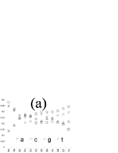
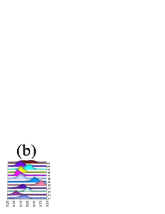
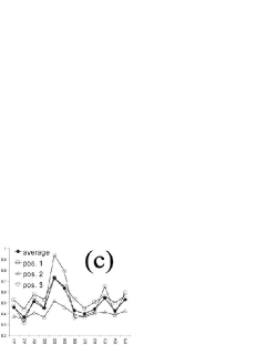
Figure 1: (a) Nucleotide frequencies. (b) Histograms for $\rho_{g+c}$. (c) $\rho_{g+c}$ in different codon positions.

Graphic 1c shows the values of $\rho_{g+c}^{j}=\rho_{c}^{j}+\rho_{g}^{j}$ for the different species, together with $\rho_{g+c}$. We notice the existence of wide variations in the $\rho_{g+c}$ composition depending on the codon position. In addition, extreme values of $\rho_{g+c}$ are usually supported by extreme values of $\rho_{g+c}^{3}$; this shows that the sequences were adapted to get a certain $\rho_{g+c}$ level, and that the third -usually synonymous- codon position was used for this purpose. As can be seen in Table 2, $\rho_{g+c}^{1}$ and $\rho_{g+c}^{2}$ are almost entirely determined by the encoded amino acids.

3.2 Codon usage

The frequency of a given codon $C=c_{0},c_{1},c_{2}\in B^{3}$ in a sequence $w=w_{0},\ldots,w_{3N-1}\in B^{3*}$ is defined as $\frac{1}{N}\sum_{i=0}^{N-1}\delta_{c_{0}}(w_{3i})\delta_{c_{1}}(w_{3i+1})\delta_{c_{2}}(w_{3i+2})$. For each codon $C\in B^{3}$, we define its synonymous class $\theta(C)=\{C^{\prime}\in B^{3}\;:\;\tau(C)=\tau(C^{\prime})\}$. Then the synonymous codon usage and the relative synonymous codon usage [29] of $C$ are defined as

$$SCU_{C}\;=\;\frac{\rho_{C}}{\displaystyle\sum_{C^{\prime}\in\theta(C)}\rho_{C}^{\prime}}\quad,\quad RSCU_{C}\;=\;\frac{|\theta(C)|\,\rho_{C}}{\displaystyle\sum_{C^{\prime}\in\theta(C)}\rho_{C}^{\prime}}\;=\;|\theta(C)|\,SCU_{C}$$

As we mentioned above, the codon choice pattern was noted very early to be a signature of the species, and our data confirm this. We will dispense with extensive SCU tables, since they are well known in the literature, and available in public databases[26]. As we said before, the common approach to backtranslation uses SCU as the probability of choosing a certain codon, given the amino acid. RSCU is used for comparisons between codons from different synonymous classes.

3.3 Dinucleotides

Most published results on dinucleotide frequencies consider long DNA sequences, including both coding and non-coding regions [4, 12, 30]. Our own computations, in spite of being limited to coding sequences, confirm most of the facts already noted by the different authors. This accounts for the fact that dinucleotide frequencies are not considered as “coding statistics”: their behavior is similar in coding and in non-coding sequences. However, they do exhibit characteristic patterns according to the different species and groups. Karlin [19] even used them to define the genome signature of a species as the collection $\{\varrho^{*}_{\alpha\beta}\}$, with $\alpha$ and $\beta$ ranging over $B$. Here $\varrho_{\alpha\beta}=\rho_{\alpha\beta}/\rho_{\alpha}\rho_{\beta}$ (with $\rho_{\alpha\beta}$ being the frequency of the dinucleotide $\alpha\beta$) and $\varrho^{*}$ is the computation of $\varrho$ over the sequence concatenated to its inverse complement (in order to get the information about both DNA strands).

IDH. There is an interesting set of indices which can be computed from dinucleotide frequencies. The so called index of DNA homogeneity (IDH) was proposed by Miramontes et al [25] and is defined for a binary sequence as $d=\frac{\rho_{00}\rho_{11}-\rho_{01}\rho_{10}}{\rho_{0}\rho_{1}}$. We define $d_{ry}(w)=d(\pi_{ry}(w))$, $d_{ws}(w)=d(\pi_{ws}(w))$, and $d_{mk}(w)=d(\pi_{mk}(w))$. This index expresses the degree of local homogeneity of the sequence: long stretches of 0 or 1 will cause $d$ to be near 1, while strong alternation will push it toward -1. The three indices $d_{ry}$, $d_{ws}$ and $d_{mk}$ are not independent, and since $\pi_{mk}$ is the least meaningful of the binary projections, the choice in [25] was to plot the species in the $(d_{ry},d_{ws})$ plane. The corresponding map with our own data is in Graphic 2a. Graphic 2b displays the distribution of the values in the sequences of some species. Both the specificity and the classificatory power of IDH can be clearly noted.

   

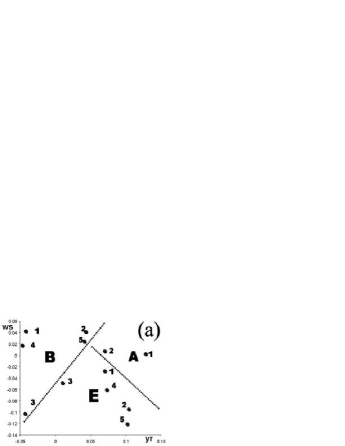
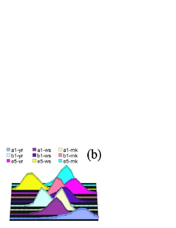
Figure 2: (a) Position of species in the $(d_{ry},d_{ws})$ plane. (b) Histograms for IDH in some species.

3.4 Fourier harmonics and Periodicities

Another common tool for DNA analysis is the discrete Fourier transform[22]. For a binary sequence $w=w_{0},\ldots,w_{N-1}$, we define the spectrum and its $m$-smoothed version:

$$S_{n}(w)\;=\;\frac{1}{N^{2}}\left|\sum_{k=0}^{N-1}w_{k}\,e^{\frac{2\,\pi\,i\,n\,k}{N}}\right|^{2}\quad\textrm{ , }\quad\tilde{S}^{m}_{n}(w)\;=\;\sum_{k=n-m}^{n+m}\frac{S_{k}(w)}{2m+1}$$

$S_{n}(w)$ measures the frequency content of ‘frequency’ $n$, which corresponds to a period $\frac{N}{n}$; the smoothed value helps to remove the dispersion that appears for small data sets.

The main and better known periodicity in DNA sequences is of period 3; it can be explained by the asymmetry in the codon positions [14, 21], though its presence in tRNA genes suggests some other origin. Another well documented periodicity is of period 10.5 $\pm$ 0.5; it has been attributed to requirements from the structure of both DNA and proteins, and the exact contribution of each is unclear. Some periodicities of higher periods have been shown, but they are not statistically significant for the typical lengths of genes.

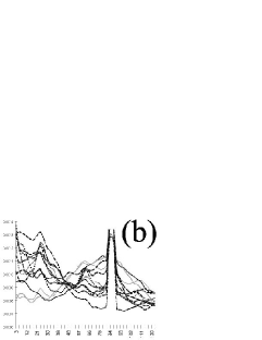
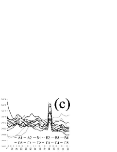
Figure 3: $\tilde{S}^{5}$ for (a) $\pi_{ws}$, (b) $\pi_{ry}$ and (c) $\pi_{mk}$.

We divided each sequence in non-overlapping windows of length 256, and used the fast Fourier transform (FFT) algorithm to compute $\tilde{S}^{5}\circ\pi_{ry}$, $\tilde{S}^{5}\circ\pi_{ws}$ and $\tilde{S}^{5}\circ\pi_{mk}$ for all the species. The results were averaged and are shown in Graphics 3a, 3b and 3c for some of the species; only part of the ordinate axis is used, in order to highlight their differences. The two periodicities mentioned before are present: there is a big peak at $n=85$ for the three projections in almost all the species (the top of the peaks is outside the graphics); this corresponds to a period of $\frac{256}{85}\approx 3$. There is also a minor peak around $n=24$, present for most species and for most projections, corresponding to the period $\frac{256}{24}\approx 10.5$; there are some differences between species, a fact that has been observed before and is related to the various origins of this periodicity.

To show the specificity of the spectrum, we chose a set of 20 collections of sequences, each set selected at random to be 1% of $E5$. We computed the average of spectra for each set; the results for $\pi_{ws}$ are shown in Graphic 4a.

Position dependent spectra. To take into account the asymmetry of the different codon positions, we computed the spectra for the three subsequences $w^{(i)}_{n}=w_{3n+i}$, $i=0,1,2$, using windows of length 64 (data not shown). In absence of period 3, the most notorious feature is a peak at $n=18$, corresponding to a period $\frac{64}{18}\approx 3.5$ in the subsequence, and hence 10.5 in the sequences; it is by far stronger for the middle codon position, a fact that hints for dependence on the amino acid sequence.

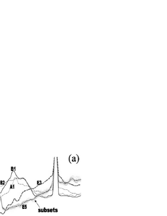
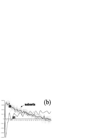
Figure 4: Dispersion of (a) $\tilde{S}^{5}$ and (b) $\tilde{\Gamma}$ for $\pi_{ws}$ in $E5$.

3.5 Autocorrelation functions

Correlation functions [13, 15] measure the excess or defect of nucleotides at different distances; if $\rho_{\alpha,\beta}(d)$ is the frequency with which we find a ‘$\beta$’ $d$ positions after a ‘$\alpha$’, then what we compute is $\rho_{\alpha,\beta}-\rho_{\alpha}\rho_{\beta}$. More precisely, what we compute for a sequence $w=w_{0},\ldots,w_{N-1}$ is

$$\Gamma_{\alpha,\beta}(d)[w]\;=\;\frac{1}{N-d}\sum_{i=0}^{N-d-1}\delta_{\alpha}(w_{i})\delta_{\beta}(w_{i+d})\;-\;\rho_{\alpha}(w)\rho_{\beta}(w)$$

We computed $\Gamma_{0,0}$ for $\pi_{ry}$, $\pi_{ws}$, $\pi_{mk}$. The most notorious result of this computation is the strong oscillation due to period 3; this can be removed by considering the smoothed version, $\tilde{\Gamma}_{\alpha\beta}(d)=\frac{1}{3}\sum_{i=d-1}^{d+1}\Gamma_{\alpha\beta}(i)$; when this was done, the periodicity of period 10.5 could also be seen. To give an idea of the shape of the curves, and to show their specificity, Graphic 4b shows the results for $\pi_{ws}$, for $B1$, $E5$, and the same subsets of $E$ used in Graphic 4a. In general, $\Gamma$ behaves very similar to the Fourier transform, in specificity and in the dependencies on alphabet and/or codon position. This is no surprising, since both express the same information (if $\Gamma$ is computed for a circular sequence, then it can be recovered form the spectra, and vice versa, by the Wiener-Khinchin theorem). Position dependent autocorrelation functions were also computed, with no unexpected results.

4 Backtranslation strategy

4.1 Genomic style beyond codon usage

We will consider all of the coding statistics reviewed in the previous section as features defining the genomic style of a species. It is important to notice that they are not (or not directly) dependent on the codon usage; if this were the case, then genomic style would reduce to RSCU, and the current approach to backtranslation would be already optimal.

It is clear that $\rho_{\alpha}$ and $\rho^{j}_{\alpha}$ are recovered by RSCU, if the amino acid composition is kept constant (this is the case in $\beta^{cu}_{B1}(B1)$ and $\beta^{cu}_{E5}(E5)$); in general, since amino acid composition is rather similar in all the different species (data not shown), we can expect nucleotide frequencies to be conserved.

For dinucleotides, this is not so clear, even if the amino acid frequencies are kept: in spite of recovering the number of dinucleotides starting at the first and second codon positions, RSCU will not recover those starting at the third. This is important, since most of the degeneracy is in this position, and “genomic style” depends strongly on it; moreover, mutation rates tend to be affected by the neighboring nucleotides [2, 16], in ways that are species-dependent. In particular, Miramontes et al [25] show that their indices (IDH) are not determined by codon usage, even when the amino acid frequency was conserved. Our data (not shown) confirm it.

As for the Fourier spectra, Guigó [10, 11] shows that it is rather independent from $\rho_{g+c}$. To discard dependence on RSCU, we computed the spectra on $\beta^{cu}_{B1}(B1)$, $\beta^{cu}_{B1}(E5)$, $\beta^{cu}_{E5}(E5)$ and $\beta^{cu}_{E5}(B1)$; results for $\tilde{S}^{5}_{n}\circ\pi_{ws}$ are displayed in Graphic 5a. We can see that all the sets of guesses lie between the real spectra, with codon usage being a bit more relevant than the amino acid sequences (the species); this was also the case for $\pi_{ry}$ and $\pi_{mk}$ (data not shown). Although the autocorrelation function contains the same information as the spectrum, the details of each one are the main lines of the other, and thus, each may be considered apart. Graphic 5b displays computations of $\tilde{\Gamma}_{0,0}\circ\pi_{ws}$ over the same sets; it can be noticed that in this case the species (amino acid sequences) are the major contribution, with only a small effect of RSCU.

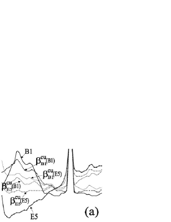
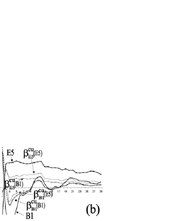
Figure 5: (a) $\tilde{S}^{5}$ and (b) $\tilde{\Gamma}$ for the $\pi_{ws}$ projection of $B1$, $E5$, $\beta^{cu}_{B1}(B1)$, $\beta^{cu}_{B1}(E5)$, $\beta^{cu}_{E5}(B1)$ and $\beta^{cu}_{E5}(E5)$.

4.2 Genetic Algorithms for Backtranslation

We want to obtain a backtranslation that imitates the genomic style of a target species as close as possible; thus, we will look for a backtranslation for which the coding statistics listed above are close to those of the target species, i.e., their distance is minimum. We choose, for $w\in B^{3*}$,

$$\begin{array}[]{c}f_{1}(w)\;=\;|\rho_{g+c}(w)-\rho^{*}_{g+c}|\qquad f_{2}(w)\;=\;\sum_{C\in B^{3}}|RSCU_{C}(w)-RSCU_{C}^{*}|\\ f_{3}(w)\;=\;|d_{ry}(w)-d_{ry}^{*}|+|d_{ws}(w)-d_{ws}^{*}|+|d_{mk}(w)-d_{mk}^{*}|\\ f_{4}(w)\;=\;\sum_{k=3}^{125}a_{k}|\tilde{S}^{5}_{k}(w)-\tilde{S}^{5,*}_{k}|\qquad f_{5}(w)\;=\;\sum_{d=2}^{99}b_{k}|\tilde{\Gamma}_{k}(w)-\tilde{\Gamma}^{*}_{k}|\end{array}$$

where the values with “*” are obtained averaging over the known coding sequences of the target species, and $a_{k}$ and $b_{k}$ are weights, incorporated in order to give more importance to some parts of the curves, e.g. to encourage a uniform convergence. The indices in the sums of $\tilde{S}$ and $\tilde{\Gamma}$ follow our particular choices of window lengths 256 and 30, respectively.

With these definitions, what we want, for a given $u\in A^{*}$ and a given target species, is to minimize $\vec{f}(w)$, with $w\in\tau^{-1}(u)$. There are two main difficulties involved. First, we have a non-convex problem, in a vast search space, with terms depending on several scales of the sequences. Moreover, it is a problem of multiobjective optimization. For these reasons, we propose the use of genetic algorithms[17] (GA), specially suited for problems with these characteristics. Our particular implementation of a genetic algorithm for backtranslation follows here.

• for $1\leq i\leq n$ initialize $w^{i}=\beta^{cu}(u)$

• while not stop condition

  • for $1\leq j\leq 5$, $\bar{f}_{j}=\max_{i}f_{j}(w^{i})$

  • for $1\leq i\leq n$, $1\leq j\leq 5$, $\displaystyle N_{j}^{i}=\frac{\bar{f}_{j}-f_{j}(w^{i})}{n\bar{f}_{j}-\sum_{k}f_{j}(w^{k})}$

  • for $1\leq i\leq n$, $N^{i}=\sum_{j}\lambda_{j}N_{j}^{i}$

  • Update $P$ using $\{N^{i}\}$ [stoch. univ. sampling]

  • Apply genetic operators: crossover and mutation

For a given $u\in A^{*}$, we iterate on a population of $n$ guesses of $\tau^{-1}(u)$, denoted by $\{w^{i}\}$. As seen in the scheme, our initial condition is the usual backtranslation (imitation of RSCU); the GA is iterated then to optimize coding statistics. $N_{j}^{i}$ are the expected number of copies of a guess in the next generation; ponderating them with $\{\lambda_{j}\}$ we combine the different objective functions, without needing to make their numeric values comparable. The genetic operators used are crossover and mutation, both adapted to maintain the encoded amino acid sequence $u$. In addition, the probability of crossover between two guesses $w^{i}$ and $w^{j}$ depends on the Hamming distance between them, making crossing between distant guesses less probable (this is introduced in order to encourage the exploration of a bigger region in search space).

A special feature of this approximation is the use of the candidate solutions (guesses) as their own encodings for the GA. Of course, this is made possible by the sequential and digital nature of genetic sequences, which were the very inspiration of GA and other forms of evolutionary computation. Obvious as it may seem, this is the only application we know about in which genetic algorithms are applied to genetic sequences.

4.3 Results of GA application

The genetic algorithm was run several times for randomly selected sequences of $B1$ and $E5$ (with the other species as target, in each case), in order to find the best values for its parameters (mutation and crossover rates, population size, etc.), for the ponderations, etc.; this was done first for each $f_{i}$, and then for the combined optimization (detailed data can be found at [1]). Even when a single function was optimized, we computed all the statistics on the resulting guesses, in order to see the effect of each statistics on the rest. Optimization of spectra and autocorrelation functions, for instance, do not have the same effect on the sequence, in spite of working with the same information. Optimization of $\tilde{S}$ causes strong oscillations in $\tilde{\Gamma}$, whereas optimization of $\tilde{\Gamma}$ alone tends to cause a flattening of $\tilde{S}$. In general, imitation of $\tilde{\Gamma}$ is the most difficult, followed by $\tilde{S}$, with $\rho_{g+c}$, $RSCU$ and specially IDH being the easier. The joint optimization of the $f_{i}$ arrived at values of each $f_{i}$ only slightly worse than those obtained in single function optimization, with the exception of $f_{4}$, which was actually better. Optimization of $\rho_{g+c}$ and $RSCU$ appeared to be almost unnecessary: when only $f_{3}$, $f_{4}$ and $f_{5}$ were considered (with $\beta^{cu}$ as initial condition), the final $\rho_{g+c}$ and $RSCU$ were still closer to the target species than the original sequence was to its own. In general, all $f_{i}$ are optimized by the genetic algorithm; it is even possible to make the periodicity of period 10.5 appear in sequences from which it was absent.

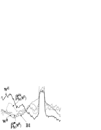
Figure 6: $\tilde{S}^{11}$ for the $\pi_{ry}$ projection of $B1$, $W^{B}$, $\beta^{cu}_{B1}(W^{E})$, $\beta^{*}_{B1}(W^{E})$ and $W^{E}$.

To remove the differences due to the amino acid sequences (which can strongly influence any coding statistic in a sample with just a few sequences), we constructed a test set with sequences encoding homologue proteins in $B1$ and $E5$. To do this, we extracted from the euGenes database [7] the list of homologies between these species, chose the cases with a higher identity percentage, and cut the segment of each sequence corresponding to the alignment. Thus we obtained a set $W^{B}=\{w^{B}_{1},\ldots,w^{B}_{20}\}$ of sequences from $B1$, and another set $W^{E}=\{w^{E}_{1},\ldots,w^{E}_{20}\}$ from $E5$, with each pair $w^{B}_{i},w^{E}_{i}$ encoding very similar amino acid sequences. We performed a canonical backtranslation on $\tau(W^{E})$, obtaining $\beta^{cu}_{B1}(W^{E})$; we perform also a backtranslation by means of our genetic algorithm, obtaining what we will call $\beta^{*}_{B1}(W^{E})$. The computation of the diverse coding statistics allows us to see how this procedure gets the backtranslation closer to the average style of $B1$; moreover, since we do have $W^{B}$, we can compare with the values of that particular set of $B1$. For instance, for IDH, we can compute a distance between two sets of sequences $S_{1}$ and $S_{2}$ as $d_{idh}(S_{1},S_{2})=|d_{ry}(S_{1})-d_{ry}(S_{2})|+|d_{ws}(S_{1})-d_{ws}(S_{2})|+|d_{mk}(S_{1})-d_{mk}(S_{2})|$. We obtain that $d_{idh}(W^{E},W^{B})=0.275$, while $d_{idh}(\beta^{cu}_{B1}(W^{E}),W^{B})=0.104$, and $d_{idh}(\beta^{*}_{B1}(W^{E}),W^{B})=0.049$. Something similar happens with the other statistics. Graphic 6 shows the graphs of $\tilde{S}^{11}\circ\pi_{ry}$ for the different sets; we can see again how $\beta^{*}$ builds a preimage for the image of $W^{E}$ (which is a typical $E5$ subset) which is far more similar to $B1$ and $W^{B}$ than the usual backtranslation procedure, $\beta^{cu}$. For $\tilde{\Gamma}$ the results are similar, but not so easy to observe in the graphics; instead of that, Table 3 displays the average difference between the curve $\tilde{\Gamma}(W^{B})$, and those for $W^{E}$, $\beta^{cu}_{B1}(W^{E})$ and $\beta^{*}_{B1}(W^{E})$. Again, $\beta^{*}$ improves with respect to $\beta^{cu}$.

Table 3: Average distance of curves $\tilde{\Gamma}$

Projection	$d(W^{E},W^{B})$	$d(\beta^{cu}_{B1}(W^{E}),W^{B})$	$d(\beta^{*}_{B1}(W^{E}),W^{B})$
$\pi_{ws}$	0.0018	0.0013	0.0008
$\pi_{ry}$	0.0016	0.0019	0.0011

5 Discussion

The purpose of this article is to propose an improvement of the current procedures of protein backtranslation, through the inclusion of coding statistics other than RSCU which contribute to characterize the different genomes; this can be accomplished by the use of genetic algorithms. We first presented several known coding statistics, showing their idiosyncratic nature. Then we proposed a particular implementation of genetic algorithms, for a small set of coding statistics; this is only an example, since other choices of the statistics, or other implementations of evolutionary computation, may give better results. Our implementation, which is available at [1], does already produce backtranslations which mimic the coding statistics of the target species, in ways that are not automatically reproduced by RSCU imitation.

The definitive test for our approach would be the use of our procedure for the in vitro generation of actual artificial genes: we expect it to have a higher success frequency than the canonical backtranslation. Meanwhile, the in silico experiment consisting in the backtranslation of a human protein into “bacterial” style, and the comparison of the statistics of the resulting gene to those of an homologue bacterial gene (see section 4.3), suggest that our approach is correct. In fact, the “optimized” preimages had more exact matches with the bacterial genes (at the aligned codon positions) than the simple RSCU-based backtranslation; this happened when human proteins were optimized for “bacterial style”, and also when bacterial proteins were translated into “human”. Though small, the systematic increase in exact matches is surprising: we did not expect the imitation of coding statistics to have this effect, since the number of preimages satisfying a given profile is still huge.

This increase in exact matches suggests that the algorithm could be also applied to the problem of “gene fishing” through PCR reactions primed by degenerate primers, or “guessmers”. This is a particular case of backtranslation, limited to short sequences selected for their minimal ambiguity. Thus, coding statistics are hard to evaluate (sequences are short) and hard to optimize (sequences are rigid). In spite of these difficulties, preliminary in silico experiments seem to support this application.

Another field of application for the ideas presented here is the analysis of sequences: discussions on the relations and origins of coding statistics can be illuminated by massive backtranslation of sequences under some criteria, like we did in 4.1 with RSCU to study its relation to spectra and autocorrelation functions. Of special interest are the comparisons between genes suspected, or known, to be related by horizontal transfer[34]. Values of RSCU and/or $\rho_{g+c}$ divergent from the style of a genome have been used to detect horizontally transferred genes; the degree of their divergence has been used as a clock to determine when a gene was acquired[33]. Some authors[20] have done this through a “reverse amelioration” which is a kind of backtranslation, and could be enriched by the results and procedures given here.

6 Acknowledgments

This research was supported by CONICYT through the FONDAP program in Applied Mathematics, and was started during a visit to the GREG (Group de Recherche et d’Etude sur les Genomes) at the Institut of Mathematics at Luminy, University of Marseille, France. Special thanks to Alejandro Maass for his lasting support.

References

-
[1]
http://www.dim.uchile.cl/
~genoma/tip
Data sets, computations, extended bibliography, and software. The source code (which is available) is very flexible, to allow interested researchers to include their own functions to be optimized. - [2] P.F. Arndt, C. Burge, T. Hwa, 2002. DNA Sequence Evolution with Neighbor-Dependent Mutation. In Proc. 6th Annual Intern. Conf. on Comp. Biol., 32–38.
- [3] D. Benson et al, 2002. Genbank. Nucl. Acids Res. 30:17–20.
- [4] C. Burge, A. Cambell, S. Karlin, 1992. Over- and under-representation of short oligonucleotides in DNA sequences. Proc. Natl. Acad. Sci. USA 89:1358–1362.
- [5] A.D. Cristillo et al, 2001. Double-stranded RNA as a not-self alarm signal: to evade, most viruses purine-load their RNAs, but some (HTLV-1, EBV) pyrimidine-load. J. Theor. Biol. 208:475–491.
- [6] D.R. Forsdyke, 1996. Different biological species “broadcast” their DNAs at different (G+C)% “wavelengths”. J. Theor. Biol. 178:405–417.
- [7] D. Gilbert, 2002. euGenes: a eukaryote genome information system. Nucl. Acids Res. 30:145–148.
- [8] R. Grantham, 1980. Workings of the genetic code. Trends Bioch. Sci. 5:327–331.
- [9] R. Grantham et al, 1986. Patterns of codon usage in different kinds of species. Oxford Surveys of Evolutionary Biology 3:48–81.
- [10] R. Guigó, J. Fickett, 1995. Distinctive Sequence Features in Protein Coding, Genic Noncoding, and Intergenic Human DNA. J. Mol. Biol. 253:51–60.
- [11] R. Guigó, 1999. DNA Composition, Codon Usage and Exon Prediction. In Genetic Databases, M.J. Bishop ed., Academic Press, 1999.
- [12] D. Häring, J. Kypr, 1999. Variations of the Mononucleotide and Short Oligonucleotide Distributions in the Genomes of Various Organisms. J. Theor. Biol. 201:141–156.
- [13] H. Herzel, I. Grosse, 1995. Measuring correlations in symbol sequences. Physica A 216:518–542.
- [14] H. Herzel, I. Grosse, 1997. Correlations in DNA sequences: The role of protein coding segments. Phys. Rev. E 55:800–810.
- [15] H. Herzel, E.N. Trifonov, O. Weiss, I. Grosse, 1998. Interpreting correlations in biosequences. Physica A 249:449–459.
- [16] S. Hess, J. Blake, R. Blake, 1994. Wide variations in neighbor-dependent substitution rates. J. Mol. Biol. 236:1022-1033.
- [17] J.H. Holland, Adaptation in Natural and Artificial Systems. The University of Michigan Press, Ann Arbor, 1975.
- [18] D. Holste et al, 2000. Optimization of Coding Potentials Using Positional Dependence of Nucleotide Frequencies. J. Theor. Biol. 206:525–537.
- [19] S. Karlin, J. Mrázek, 1997. Compositional differences within and between eukaryotic genomes. Proc. Natl. Acad. Sci. USA 94:10227–10232.
- [20] J. Lawrence, H. Ochman, 1997. Amelioration of bacterial genomes: Rates of change and exchange. J. Mol. Evol. 44:383–397.
- [21] W. Lee, L. Luo, 1997. Periodicity of base correlation in nucleotide sequences. Phys. Rev. E 56:848–851.
- [22] V.V. Lobzin, V.R. Chechetkin, 2000. Order and correlations in genomic DNA sequences. The spectral approach. Physics - Uspekhi 43:55–78; available at http://ufn.ioc.ac.ru/Index00.html.
- [23] J. Ma et al, 2002. Cluster analysis of the codon use frequency of MHC genes from different species. Biosystems 65:199–207.
- [24] G. Macaya, J.P. Thiery, G. Bernardi, 1976. An approach to the organization of eukaryotic genomes at a macromolecular level. J. Mol. Biol. 108:237–254.
- [25] P. Miramontes et al, 1995. Structural and Thermodynamic Properties of DNA Uncover Different Evolutionary Histories. J. Mol. Evol. 40:698–704.
- [26] Y. Nakamura et al, 1999. Codon usage tabulated from the international DNA sequence databases; its status 1999. Nucl. Acids Res. 27:292.
- [27] M. Nashimoto, 2001. The RNA/Protein Symmetry Hypothesis: Experimental Support for Reverse Translation of Primitive Proteins. J. Theor. Biol. 209:181–187.
- [28] G. Pesole et al, 1988. A backtranslation method based on codon usage strategy. Nucl. Acids Res. 16:1715–1728.
- [29] P.M. Sharp, W.H. Li, 1987. The codon adaptation index - a measure of directional synonymous codon usage bias, and its potential applications. Nucl. Acids Res. 15:1281–1295.
- [30] C. Shioiri, N. Takahata, 2001. Skew of mononucleotide frequencies, relative abundance of dinucleotides, and DNA strand asymmetry. J. Mol. Evol.53:364–376.
- [31] A. Smith et al, 1990. Expression of a Synthetic Gene for Horseradish Peroxidase C in Escherichia coli and Folding and Activation of the Recombinant Enzyme with and Heme. J. Biol. Chem. 265:13335–13343.
- [32] R. Staden, A. McLachlan, 1982. Codon preference and its use in identifying protein coding regions in long DNA sequences. Nucl. Acids Res. 10:141–156.
- [33] N. Sueoka, 1993. Directional mutation pressure, mutator mutations, and dynamics of molecular evolution. J. Mol. Evol. 37:137–158.
- [34] M. Syvanen, C.I. Kado, eds, Horizontal Gene Transfer. Chapman & Hall, London, 1998.
- [35] E.N. Trifonov, 1998. 3-, 10.5-, 200- and 400-base periodicities in genome sequences. Physica A 249:511–516.
- [36] G. White, W. Seffens, 1998. Using a neural network to backtranslate amino acid sequences. Electronic Journal of Biotechnology 1:3.