Present address: ]Physics Department, University of Colorado, Campus Box 390, Boulder ,CO, 80309

Tests for non-randomness in quantum jumps

Abstract

In a fundamental test of quantum mechanics, we have observed 228 000 quantum jumps of a single trapped and laser cooled ⁸⁸Sr⁺ ion. This represents a statistical increase of two orders of magnitude over previous similar analyses of quantum jumps. Compared to other searches for non-randomness in quantum mechanical processes, using quantum jumps simplifies the interpretation of data by eliminated multi-particle effects and providing near-unit detection efficiency of transitions. We measure the fractional reduction in the entropy of information to be $<6.5~{}10^{-4}$ when the value of any interval between quantum jumps is known. We also find that the number of runs of successively increasing or decreasing interval times agrees with the theoretically expected values. Furthermore, we analyze 238 000 quantum jumps from two simultaneously confined ions and find that the number of apparently coincidental transitions is as expected. Finally, we observe 8400 spontaneous decays of two simultaneously trapped ions and find that the number of apparently coincidental decays from the metastable state agrees with the expected value. We find no evidence for short- or long-term correlations in the intervals of the quantum jumps or in the decay of the quantum states, in agreement with quantum theory.

An axiom of quantum mechanics is that we cannot predict the result of any single measurement of an observable of a quantum mechanical system in a superposition of eigenstates. Testing this principle is important, not only for basic science, but also for applications such as quantum random number generators (QRNG’s) and potential quantum computers. It is therefore surprising that in spite of the many experiments sensitive to quantum mechanical effects, only a few experiments have explicitly searched for non-random behavior in long sequences of repeated quantum measurements. In Thomas:2000 ; Andre:2000 , the randomness of the path of a single photon after a beamsplitter was used to build QRNG’s. In  Silverman:1999 , the arrival times of decay products of unstable nuclei were used to test the statistics of quantum decay. Although both these systems rapidly give excellent statistics, detector inefficiencies limit the conclusions that can be drawn regarding the unpredictability of quantum mechanical measurements. Furthermore, both systems are insensitive to certain types of non-random behavior: averaging over many particles in a collection of nuclei could obscure non-random behavior of single systems, patterns in emission times or photon arrival times could be overlooked because of inefficient detectors, and because beamsplitters are always somewhat biased, QRNG’s based on them are designed to be insensitive to consecutive runs of transmissions or reflections. All these problems can be avoided by observing the times of quantum jumps in a single atom Cook:1990 because transitions between atomic levels can be detected with near-unit efficiency with no multi-particle effects Erber:1985 .

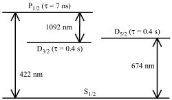
Figure 1: Partial energy level diagram, transitions and lifetimes in ⁸⁸Sr⁺. We drive the 422-nm transition to Doppler cool and detect the ions, and the 1092-nm transition to prevent optical pumping into the D_3/2 state. A laser of bandwidth $<10$ kHz drives the 674-nm transition to produce quantum jumps to and from D_5/2 states.

Here, we analyze the intervals between quantum jumps of a trapped ion and answer the question “after we have measured the length of one interval, how much have we decreased the uncertainty of the value of any interval we subsequently measure?” This question is directly relevant to quantum logic operations on any quantum mechanical system Galindo:2002 ; if the result of one logic operation affects that of subsequent (and supposedly independent) operations then the operation of the gate is compromised. It is also critical for demonstrating the suitability of a quantum mechanical system as a random number generator.

Earlier work Erber:1989 examined 640 quantum jumps in a single ¹⁹⁸Hg⁺ ion confined in a Paul trap Bergquist:1986 . Ref. Erber:1995 later reported a different but limited analysis of 10 000 quantum jumps. In a substantial increase in statistics over this previous work, we analyze 228 000 quantum jumps from a single ion comprising continuous data sets of $\sim$10 000 events each. We take advantage of our greater statistics to also test for unexpected correlations between transition times of multiple ions, analyzing 238 000 quantum jumps and 8400 spontaneous decays of pairs of trapped ions.

We confine ⁸⁸Sr⁺ ions in a linear Paul trap Berkeland:2002 and simultaneously drive the transitions shown in Fig. 1. Figure 2 shows a sample of the measured 422-nm scattering rate as a function of time. It displays the well-known characteristics of quantum jumps: the ion rapidly scatters resonant 422-nm light when it is in the S${}_{1/2}\leftrightarrow$ P${}_{1/2}\leftrightarrow$ D_3/2 manifold, but not at all when it is in one of the metastable D_5/2 magnetic sub-levels. The scattering rate changes abruptly whenever a 674-nm photon is absorbed or emitted. According to quantum theory, the exact times of these changes, and the intervals between them, should be unpredictable.

To test this assumption, we analyze the number of 422-nm photons that scatter from the ion and reach a photomultiplier tube in a measurement time $t_{meas}$ (typically a few ms, followed by a 200 $\mu$s dead time) when all three transition in Fig. 1 are simultaneously driven. Each data set of approximately 10 000 measurements is taken over approximately 30 minutes. From these data we obtain four series $U=\{u_{1},u_{2},u_{3},\ldots,u_{N}\}$ of sequential time intervals, defined as follows. We label as “bright” the series of intervals during which the ion continuously scatters 422-nm light, and “dark” the series of intervals during which the ion fluorescence is continuously absent. In addition we analyze the series of intervals between successive emissions (“emission”) and absorptions (“absorption”) of a 674-nm photon.

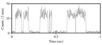
Figure 2: Number of 422-nm photons counted by the detector over time, when all of the transitions shown in Fig. 1 are driven simultaneously.

Before each data set, we adjust the intensities of the laser beams to control the rate of quantum jumps. The bright intervals are distributed exponentially, with average values ranging from 70 to 200 ms, while the average values for dark intervals range from 30 to 150 msec. When integrated over the long times of a data set, the distributions of dark intervals deviate slightly from a purely exponential form for interval durations greater than 100 msec. This is due to drifts in the frequencies and intensities of laser light at the site of the ion, which cause slight variations in the average bright and dark interval durations. In addition, in the presence of a degeneracy-breaking magnetic field $B$ (we vary $B$ from  $10^{-6}$ T to $2~{}10^{-4}$ T), transitions from each D_5/2 Zeeman sub-level contribute distinct exponential distribution to the distribution of dark intervals. In spite of their different responses to these two effects, the dark and bright intervals in our experiment give statistically identical results. We conclude from this that these effects neither introduce nor mask correlations between intervals on the time scales of our statistical tests.

Previous studies of randomness in quantum mechanics have used several algorithms for answering the question regarding predictability of intervals posed at this beginning of this paper: for example, analyzing the distribution of sums and differences of intervals Erber:1989 , verifying that the probability of particle decay is constant over short and long time-scales Silverman:1999 , and analyzing lengths of continuously increasing and decreasing runs of intervals Silverman:1999 ; Erber:1989 . We calculate the difference between the entropy and conditional entropy of sets of intervals, because this directly answers our question, and because it results in an upper limit on the association of adjacent and non-adjacent pairs of intervals.

To do this, we first divide our data sets into continuous strings of 1000 events and normalize each interval time by the average interval time of its string. This nearly eliminates effects due to slow drifts of the rate of quantum jumps. Using each interval $u_{i}$ only once, for $k\geq 1$ we tabulate the number of occurrences $N_{m,n}$ of pairs {$u_{i}$, $u_{i+k}$} for which $u_{i}\in[t_{m},t_{m+1})$ and $u_{i+k}\in[t_{n},t_{n+1})$. We choose $t_{m(n)}$ at intervals that result in roughly uniform values of $N_{m,n}\gg 1$ for all $\{m,n\}$, although we find that our results do not depend on the degree of uniformity. We set the number of bins in each row and column ($m_{max}=n_{max}$) to be 13.

Next, following Press Press:1989 we call $p_{m\cdot}$ the probability that the first interval in a pair ($u_{i}$) lies within the range $[t_{m},t_{m+1})$, and $p_{\cdot n}$ the probability that the second interval ($u_{i+k}$) lies in the range $[t_{n},t_{n+1})$. We also call $p_{m,n}=N_{m,n}/N$ (where $N$ is the total number of pairs) the probability that the pair falls in bin $\{m,n\}$. The entropies are then defined as

$$H(x)=-\sum\limits_{n}p_{\cdot n}~{}ln~{}p_{\cdot n}$$ (1)

$$H(y)=-\sum\limits_{m}p_{m\cdot}~{}ln~{}p_{m\cdot}~{},$$ (2)

and the conditional entropies are then defined as

$$H(x|y)=-\sum\limits_{m,n}p_{m,n}~{}ln~{}(p_{m,n}/p_{m\cdot})$$ (3)

$$H(y|x)=-\sum\limits_{m,n}p_{m,n}~{}ln~{}(p_{m,n}/p_{\cdot n})~{}.$$ (4)

These define two joint measures of the association between the first and second intervals of any pair:

$$U(x|y)=\frac{H(x)-H(x|y)}{H(x)}$$ (5)

$$U(y|x)=\frac{H(y)-H(y|x)}{H(y)}~{}.$$ (6)

$U(x|y)$ represents the amount of information that the distribution of first intervals gives about the distribution of second intervals Press:1989 , and vice versa for $U(y|x)$. For an infinitely large data set, if the intervals in a pair are statistically independent of each other then $U(x|y)=U(y|x)=0$, and if they are completely associated with each other, $U(x|y)=U(y|x)=1$. However, statistical fluctuations in the $N_{i,j}$’s limit how closely $U(x|y)$ and $U(y|x)$ approach 0.

Figure 3 shows $U(x|y)$ and $U(y|x)$ as functions of the number of intervals $k$ that separate each pair $\{u_{i},u_{i+k}\}$ for the four different interval types. The values do not depend on $k$. Figure 4 shows the average values of $U(x|y)$ and $U(y|x)$. They are consistent with each other and with the value 0.00062 that is calculated if all of the $N_{m,n}$ were randomly distributed about the average value $q=N~{}m^{-2}_{max}$ with a distribution width $\sqrt{q}$. These facts show that intervals are uncorrelated when they are separated by 1 to 20 intervals, which corresponds to approximately 2 ms to several seconds.

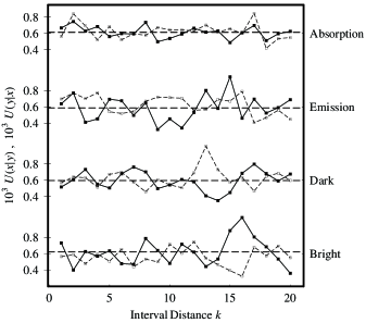
Figure 3: The joint functions $U(x|y)$ (solid lines) and $U(y|x)$ (dashed lines) from Eqs. 5 and 6 as a function of the number of intervals between pairs for bright and dark intervals and intervals between emissions and absorptions of 674-nm photons. Heavy dashed lines indicate the average values for each interval type.

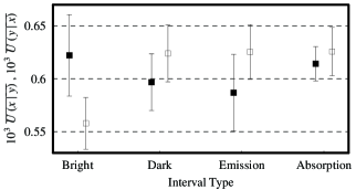
Figure 4: The average values of $U(x|y)$ (solid boxes) and $U(y|x)$ (hollow boxes) from Fig. 3.

As a complimentary test for short- and long-term order, we search for deviations from the expected distribution of consecutively increasing or decreasing runs of elements of length $m$. As an example, the subsequence $\{\ldots,3,15,11,5,7,2\ldots\}$ contains a run down of three elements (15, 11 and 5) and a run up of two elements (5 and 7). If the data set $U$ has a total of $N$ elements, the expected number of runs up or down of length $\ell$ is Erber:1989

$$N_{runs}\left({\ell}\right)={\frac{{N\left({\ell^{2}+\ell-1}\right)+\ell\left({4-\ell^{2}}\right)+1}}{{\left({\ell+2}\right)!}}}~{}.$$ (7)

This equation assumes that no element in $U$ is repeated. However, we measure the intervals $u_{i}$ in integer multiples of $t_{meas}$. Often a run is terminated by a repeated interval value, although it is equally likely that the run should continue. We account for such cases by tallying two run lengths, each with half the weight of a single run. We make similar adjustments when an interval occurs three times in a row. We combine all of the data to obtain $N_{runs}(\ell)$ and their deviation from the expected values, shown in Fig. 5. Because the $N_{runs}(\ell)$ are not independent of each other, a $\chi^{2}$ test does not apply. However, each point in the figure is within reasonable agreement with the expected values.

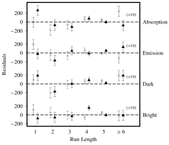
Figure 5: Differences between the expected and measured values of the number of runs up (squares) and down (triangles) for the four interval types. The values of the number of runs of length $\ell\geq 6$ have been magnified, and the runs up and down have been slightly offset along the x-axis for clarity. In total, each data set has $\sim$ 57 000 runs of various lengths both up and down.

A critical assumption in quantum algorithms involving multiple quantum systems is that in the absence of intentionally applied coupling, the individual systems do not communicate with each other. We do not expect to observe cooperative effects in the transitions times of pairs of atoms. However, other workers have seen many more apparently simultaneous quantum jumps Sauter:1986 and spontaneous decays Block:1999 than expected. We take advantage of our statistics and search for signs that transitions in ions stored simultaneously in the trap are correlated.

We analyze 248 000 quantum jumps in two ions separated by $\geq 20~{}\mu m$, and count the number of times in which both ions appear to change state during the same measurement time $t_{meas}$. In such events, the number of detected 422-nm photons $n_{422}$ in one measurement time is less than a threshold consistent with no ions fluorescing, and is immediately followed or preceded by a value of $n_{422}$ that is greater than a threshold consistent with two ions fluorescing. The probability of such events is determined by the probability per unit time for a single ion to change states, the average 422-nm photon scattering rate per ion, the two threshold values and the measurement time $t_{meas}$. We also account for the possibility of misinterpreting the scattering rate from a single ion for that of two ions due to insufficient resolution between the count rate distributions of one and two ions. The total number of coincidental transitions into the D_5/2 states is expected to be 308, and we measure 320. Also, a total of 316 coincidental transitions out of the D_5/2 states is expected from our data, and we measure 313. In addition, we find that the observed numbers agree with those produced in Monte Carlo simulations of the data.

We also analyze the spontaneous decay of simultaneously trapped ions, which may be more sensitive to effects such as interactions with background gas. A brief ($\leq$ 0.2 s) saturating pulse of 674-nm light excites the atoms to the D_5/2 states while the 422-nm light is absent. After the 674-nm light pulse, the 422-nm light is returned and we monitor the 422-nm photon scattering rate every $t_{meas}$ = 5 msec. We observe 8400 decay processes that start with two ions in the D_5/2 state and finish with no ions in the D_5/2 state. In total, 26 of these transitions appear to occur during the same measurement time $t_{meas}$. From a measured decay rate of 410 msec in our system, we expect to see 24 (4) of these processes. This, too, is consistent with the behavior of the ions being random, and agrees with the results of Steane:2000

In conclusion, while it is impossible to prove randomness, we have seen no signs of non-random behavior over short and long time scales after analyzing 228 000 quantum jumps in single ions, 238 000 quantum jumps in two simultaneously trapped ions, and 8400 spontaneous decays of two ions. Practical QRNG’s and quantum computers would use fewer quantum interactions than those analyzed here. The present sensitivity is sufficient to show that these applications are not affected by correlations due to non-randomness of quantum mechanics. However, at times short compared to the transit time of light across the ion Enaki:1996 , and times long compared to the decay rate of the atomic state  Milonni:1994 , the Weisskopf-Wigner approximation breaks down so that the distribution of decay times is no longer exponential. In this case, we would expect to see non-random behavior in the interval times of quantum jumps. Observations in these regimes are out of the reach of modern experiments, but are an intriguing possibility for future work.

This work was funded by DOE through the LDRD program. We would like to thank Malcolm Boshier for carefully reading this manuscript and for valuable discussions, and Richard Hughes for initially bringing this topic to our attention.

References

- (1) T. Jennewein, U. Achleitner, G. Weihs, H. Weinfurter and A. Zeilinger, Rev. Sci. Inst. 71, 1675-1680 (2000).
- (2) A. Stefanov, N. Gisin, O. Guinnard, L. Guinnard and H. Zbinden, J. Mod. Opt. 47, 595-598 (2000).
- (3) (a) M. P. Silverman, W. Strange, C. Silverman, and T. C. Lipscombe, Phys. Rev. A. 61, 042106 (2000); (b) M.P. Silverman and W. Strange, Phys. Lett. A 272, 1-9 (2000).
- (4) R. Cook, in Progress in Optics XXVII, ed. E. Wolf (Elsevier Science Publishers, B.V., 1990), pp. 362-416.
- (5) T. Erber and S. Putterman, Nature 318, 41-43 (1985). Academic Press, Inc., Boston, 1994, p. 148.
- (6) T. Erber, P. Hammerling, G. Hockney, M. Porrati and S. Putterman, Ann. Phys. 190, 254-309 (1989).
- (7) J.C. Bergquist, R.G. Hulet, W.M. Itano and D.J. Wineland, Phys. Rev. Lett. 57, 1699-1702 (1986).
- (8) T. Erber, Ann. N.Y. Acc. Sci. 755, 748-756 (1995).
- (9) A. Galindo and M.A. Martín-Delgado, Rev. Mod. Phys. 74, 347-423 (2002).
- (10) D.J. Berkeland, Rev. Sci. Inst. 73, 2856-2860 (2002).
- (11) W.M. Itano, J.C. Bergquist, F. Dietrick, and D.J. Wineland, in Coherence and Quantum Optics VI, ed. J.H. Eberly et al. (Plenum Press, New York, 1990), pp. 539-543.
- (12) W.H. Press, B.P. Flannery, S.A. Teukolsky and W.T. Vetterling, Numerical Recipies (FORTRAN version), Cambridge Univerisity Press, Cambridge, 1989), p. 482.
- (13) Th. Sauter, R. Blatt, W. Neuhauser and P.E. Toschek, Opt. Comm. 60, 287-292 (1986).
- (14) M. Block, O. Rehm, P. Seibert and G. Werth, E.P.J.D. 7, 461-465 (1999).
- (15) C.J.S. Donald, D.M. Lucas, P.A. Barton, M.J. McDonnell, J.P. Stacey, D.A. Stevens, D.N. Stacey and A.M. Steane, Europhys. Lett. 51, 388-394 (2000).
- (16) N.A. Enaki, JETP 82, 607-615 (1996).
- (17) P.W. Milonni, The Quantum Vacuum, (Acedemic Press, Inc., Boston, 1994), pp. 144-148.