Stochastic dynamics of the magneto-optical trap

Abstract

The cloud of cold atoms obtained from a magneto-optical trap is known to exhibit two types of instabilities in the regime of high atomic densities: stochastic instabilities and deterministic instabilities. In the present paper, the experimentally observed stochastic dynamics is described extensively. It is shown that it exists a variety of dynamical behaviors, which differ by the frequency components appearing in the dynamics. Indeed, some instabilities exhibit only low frequency components, while in other cases, a second time scale, corresponding to a higher frequency, appears in the motion of the center of mass of the cloud. A one-dimensional stochastic model taking into account the shadow effect is shown to be able to reproduce the experimental behavior, linking the existence of instabilities to folded stationary solutions where noise response is enhanced. The different types of regimes are explained by the existence of a relaxation frequency, which in some conditions is excited by noise.

1 Introduction

Magneto-optical traps (MOT) produce clouds of cooled atoms at temperature as low as the $\mu$K. The achievement of such clouds opened many perspectives, not only in the field of fundamental atomic physics, as e.g. in the domain of the atomic dynamics or the quantum chaosQC , but also leads to several potential applications, in particular the improvement by several orders of magnitude of the atomic clockclocks . The MOT is also the first stage to produce lower temperatures, in particular to obtain Bose-Einstein condensates nobel . Although the use of MOTs is relatively well mastered, some details of the experimental setup remain empirical, because of the existence in the cloud of instabilities that are not well understood. Some studies showed that when the trapping beams are misaligned, the cloud may be spatially altered and become unstable. In particular, ring-shaped clouds and chaos have been observed, and attributed to a vertex force shadow ; mis . However, the main instabilities encountered in the experiments concern well-aligned MOTs. In that case, the cloud, which is usually more or less ellipsoidal, has a complex irregular shape, with an inhomogeneous atomic density (fig 1). This shape may not be stable, and changes as a function of time: a typical example of these instabilities is shown in fig. 1.

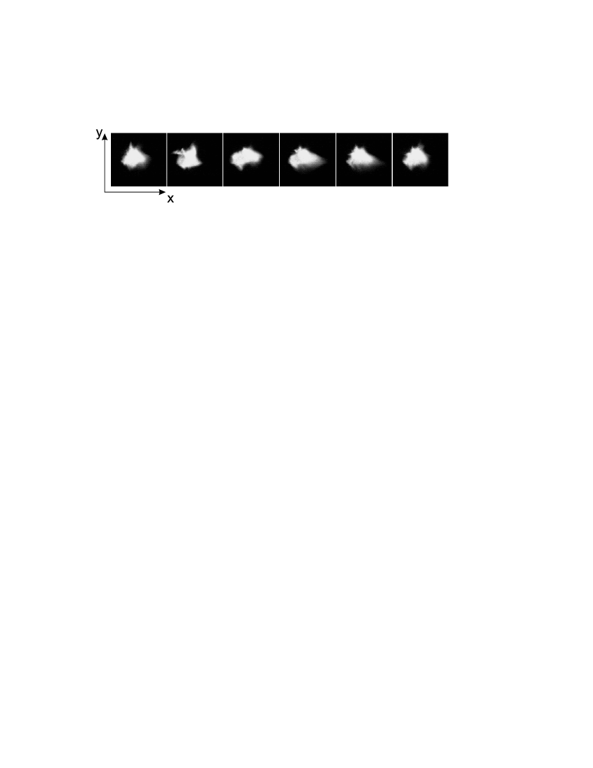
Figure 1: Sequence of snapshots showing the time evolution of the unstable atomic cloud. Snapshots are presented in the chronological order, each one being separated by 120 ms.

There is a deep interest to identify the nature of these instabilities, in the aim to control them, and possibly to take advantage of them. To illustrate these points, let us remember that instabilities may originate in many mechanisms, which can be classified in two families: stochastic or deterministic. In the latter, called also deterministic chaos, the dynamics is described by a set of deterministic equations. When the number of equations is small (low-dimensional deterministic chaos), it has been shown that the dynamics can be controlled to reach various states that are not accessible otherwise, as unstable statescontrolstab or periodic behaviorscontrolper . It is also well known that the description of such a dynamics gives access to numerous parameters, which are not measurable when the behavior is stationaryparamaccess . The cost for these informations is that there is no other way to reduce the instabilities. On the contrary, if the origin of the instabilities is stochastic, i.e. due to external noise, a reduction of instabilities is obtained by reducing the noise, but the instabilities have no physical meaning, in that sense that they are not intrinsic to the physics of the system.

In nousprl , a first type of instabilities, arising for low beam intensities, has been depicted. It was showed that these so-called “stochastic instabilities” are induced by the absorption of the trapping beams in the cloud. A model taking into account this so-called shadow effect showed that from a dynamical point of view, instabilities arise through a stochastic resonancelike phenomenon, namely the coherent resonance, linked to a Hopf bifurcation in the stationary solutions of the MOT. It is well known that such a bifurcation usually leads to periodic instabilities, and indeed, a recent study evidenced such instabilities, purely deterministic InstDet . However, a correct description of these self-oscillations required to modify the model in nousprl , in particular to take into account the spatial distribution of the cloud.

In the present paper, the results presented in nousprl are detailed, and extended to a larger range of parameters, where new regimes appear, in particular a behavior without resonance frequency, contrary to the instabilities described in nousprl . Then the modified model introduced in InstDet is accurately described, and the relative domains of appearance of stochastic and deterministic instabilities are discussed. The difference appears to be the result of the preeminent role of noise in some parameter range, in particular in the vicinity of the bifurcations. The stochastic instabilities predicted by the model are studied, and they are shown to be in agreement with those experimentally observed. In particular, an interpretation  of the two types of stochastic instabilities, with and without resonance frequency, is found.

The paper is organized as follows. After this introduction, the section 2 describes the experimental setup. Then, a detailed analysis of the experimental observations of the stochastic instabilities is presented (section 3), showing in particular the existence of two types of instabilities. Section 4 is devoted to the construction of a simple 1D model, already presented in InstDet in a less detailed way. In section 5, the stationary solutions of the model are discussed. Finally, in section 6, the noise induced dynamics instabilities is studied and compared to the experimental observations.

2 Experimental set-up

We work with a Cesium-atom MOT in the usual $\sigma_{+}-\sigma_{-}$ configuration, with three arms of two counter-propagating beams obtained from the same laser diode. The waist $w_{T}$ of the trap beams may be varied from typically $3$ to $10$ mm. Two configurations are possible: in the first one, all six beams are independent, by opposition to the second configuration, where counter-propagating beams result from the reflection of the three forward beams. In the last case, the intensity asymmetry resulting from the absorption of the forward beam by the cloud, generates a center-of-mass motion, while in the first case, instabilities are characterized by symmetrical bursts on the cloud shape, much more difficult to measure. However, as the nonlinearities involved in both cases are the same, we expect that the dynamics will be fundamentally of the same nature, and thus we choose the configuration with retro-reflected beams.

A full description of the unstable dynamics of the atomic cloud will be presented in the next section. However, to make easier the understanding of this paragraph, let us depict them briefly. As shown in the introduction (fig. 1), instabilities consist in a deformation of the spatial atomic distribution, leading to fluctuations of the shape of the cloud. Therefore, the relevant dynamical variables allowing us to describe instabilities, could be the shape of the cloud (i.e. for example the local velocities and atomic densities in the cloud). This type of description corresponds to a high dimensional model, associated with partial differential equations. Here, for the sake of simplicity, we choose to limit our description to the center of mass (CM) location ${\bf r}$, and the total number of atoms $n$ in the atomic cloud. This allows us to model the system with ordinary differential equations, and reduces the dimension to seven, and even three in a 1D model. As it is shown in the following, the use of this description appears to be sufficient to understand the main mechanisms of the instabilities.

To measure ${\bf r}$ and $n$, we used two 4-quadrant photodiodes (4QP) forming an orthogonal dihedral and measuring the fluorescence of the cloud. The differential signal of the 4QP allows us to monitor the motion of the CM. Using only two 4QPs does not allow us to reconstruct the actual 3D motion, but gives access to projections of this motion on two different axes. This prevents the measure from line-of-sight effects due to the optical thickness of the cloud. We checked that whatever the type of dynamical behavior, the motion components $r$ recorded by both 4QP have the same properties and are qualitatively identical. In the following, the “CM motion” refers to a component $r$ of this motion recorded by one of the 4QPs. The second dynamical variable, namely the number of atoms inside the cloud, is deduced from the total signal received from the 4QPs. In addition to the 4QPs, two video cameras monitor the shape of the cloud. Because of their poor resolution as compared with the 4QPs, the video cameras are not used to record the dynamical variables. They have been essentially used in the first stages of the experiment, to control that there is no discrepancy between the shape dynamics and the CM dynamics.

Instabilities depend on the MOT parameters. Among these parameters, some are easily controllable, and will be referred in the following as control parameters. They are the detuning $\Delta_{0}$ of the MOT, the magnetic field gradient $G$, the MOT beam intensities $I_{1}$ and the repumper laser intensity $I_{rep}$. Other parameters cannot be considered as control parameters, because they are not easily controllable or measurable in our experimental setup. Among these parameters, the alignment of the MOT beams appeared to be crucial in the experiment. We limit the present study to the case where beams are aligned. When misaligned, most of the dynamical characteristics of the cloud change qualitatively mis . The MOT beam waists play also a main role on the dynamics, but in practice, they cannot be changed easily independently from the other parameters, in particular $I_{1}$. However, two different values have been used in the experiments, and their effects on the dynamics are well understood. Finally, the vapor pressure in the cell has probably also a large influence on the dynamics. Unfortunately, this parameter is not easily measurable in our experimental setup. Moreover, as it is shown later, it does not appear explicitly in the model, but its impact on the dynamics may be estimated through the equilibrium population of the cloud. The parameter ranges explored in the present experiment are summarized in Tab. 1.

Table 1: Range of the parameters used in the present experiment. $G$ is the magnetic field gradient, $I_{1}$ is the intensity of the forward beam, $\Delta_{0}$ is the detuning and $w_{T}$ is the trap laser beam waist. $I_{s}$ is the saturation intensity ( $I_{s}=1.1$ mW) and $\Gamma$ is the natural width of the transition. The last column indicates the default parameter values used to obtain the results reported in the present paper.

	range	default set
$G$ (Gcm-1)	$G\leq 14$	14
$I_{+}=I/I_{s}$	$4\leq I_{+}\leq 20$	6
$w_{T}(mm)$	$3\leq w_{T}\leq 10$	3
$\Delta_{0}$	$\Delta_{0}\leq-0.5$	-

3 Experimental results

Instabilities have been described in nousprl for a given set of parameters. In the following, we extend this description for the whole range of parameters where stochastic instabilities appear. A first fundamental control parameter is the MOT beam intensity, whose value determines the type of observed instabilities. At low MOT beam intensities, typically less than $10I_{S}$ ($I_{S}=1.1$ mW/cm² is the saturation intensity), the cloud exhibits S instabilities (S stands for Stochastic). For MOT beam intensities larger than $10I_{S}$, C (for Cyclic) instabilities appear InstDet . As the aim of the present paper is to discuss about the stochastic instabilities, we keep a detailed presentation of the deterministic C instabilities for another paper. However, the two types of instabilities cannot be completely separated, and the domains of appearance of both types of instabilities will be discussed.

As discussed above, S instabilities appear at low MOT beam intensities, and are characterized by large fluctuations of the shape of the cloud appearing in a limited range of the parameters. From the experimental point of view, this last point is essential, because it is at the origin of the introduction of the concept of instabilities of the MOT. Indeed, if the noisy dynamics is the same whatever the parameter values, it is clear that the problem becomes as trivial as the reduction of technical noise in an experiment. On the contrary, the motion of the MOT grows suddenly in a narrow range of the parameters, as it is illustrated in fig. 2, where the amplitude $\Delta r$ of the $r$ fluctuations is represented as a function of the control parameter $\Delta_{0}$. Far from the unstable area, e.g. at large $\left|\Delta_{0}\right|$, the cloud is stable in shape and density. When the control parameter is tuned to the unstable area, instabilities appear progressively, and the amplitude grows until a maximum $\Delta r_{\max}$ at $\Delta_{0\max}\simeq-1.95$ ($\Delta_{0}$ is expressed in units of the natural width $\Gamma$ of the atomic transition). There is no abrupt boundary between the stable and unstable areas: the limits given below corresponds to $\Delta r=\Delta r_{\max}/10$. In this case, for the set of parameters of fig. 2, instabilities appear for $-2.5<\Delta_{0}<-1.7$ (for $\Delta_{0}>-1.7$, the population in the cloud vanishes). The unstable range depends on the other parameters, such as the beam intensities, the vapor pressure or the magnetic field gradient. For example, for a less populated cloud, due e.g. to a different vapor pressure in the cell, all other parameters being the same as previously, instabilities will appear at smaller detuning. However, whatever the parameters used in the experiments, in the range given in Tab. 1, we have $-3\lesssim\Delta_{0\max}\lesssim-1$, and instabilities never occur on a range larger than $1$.

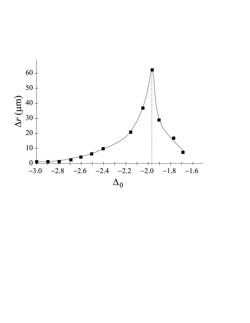
Figure 2: Evolution of the signal amplitude $\Delta r$ as a function of the detuning $\Delta_{0}$. Parameters are those of the default set of Tab. 1.

Fig. 3 shows a typical unstable behavior of $r$. It appears as an erratic signal, with a flat spectrum (fig. 4). Low frequency significant components appear typically for values smaller than $\nu_{n}\approx 2$ Hz (fig. 4b), and the dynamics is essentially along the first bisector of the three forward beams. The behavior of $r$ and $n$ are similar, with a cross correlation coefficient larger than 0.8. To determine if these instabilities have a deterministic origin, several tools are offered through the nonlinear dynamical analysis of the time series. As the MOT is dissipative, a deterministic dynamics should have an attractor, which can be reconstructed easily for a low dimensional dynamics. The result, not presented here, appears as a set of randomly distributed points: in particular, it does not present any fine structure. Poincaré section and 1D maps confirm this absence of order in the dynamics. This could be due to a lack of resolution of the measures, but the general shape of the trajectories rather suggests that the behavior is stochastic (or chaotic with a high dimensional dynamics). Because this behavior appears to be a stochastic dynamics with only low frequency components, it will be referred in the following as S_L instabilities.

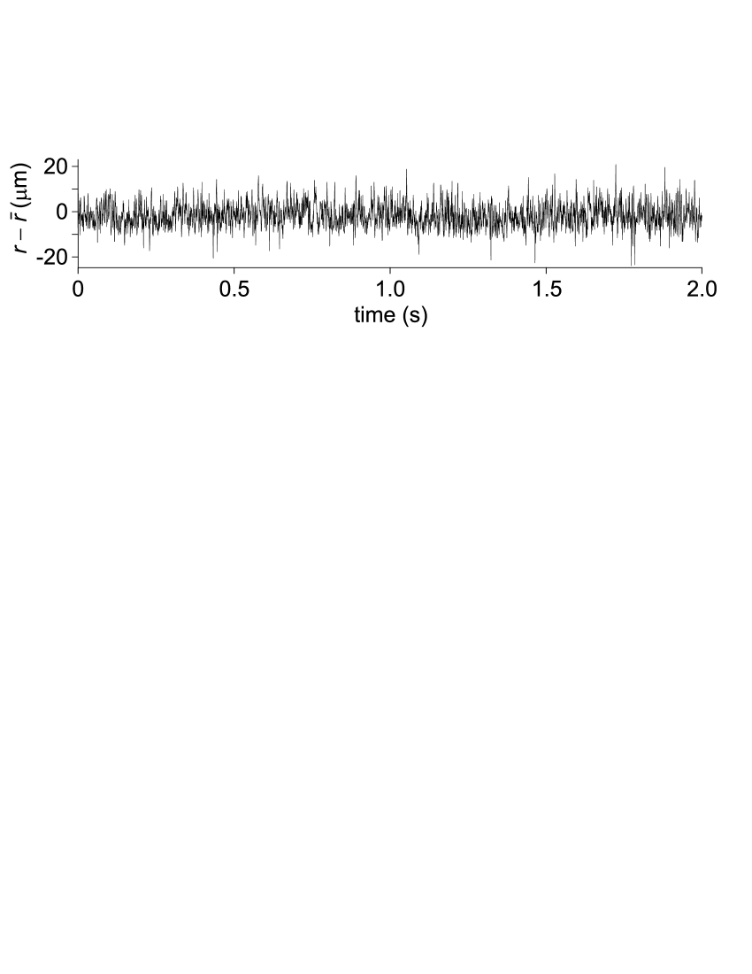
Figure 3: Experimental record of the time evolution of a component of the CM location of the atomic cloud. Experimental parameters are the default ones given in Table 1, with $\Delta_{0}=-2$. The mean cloud population is $1.5\times 10^{8}$ atoms and the cloud size is 1 mm.

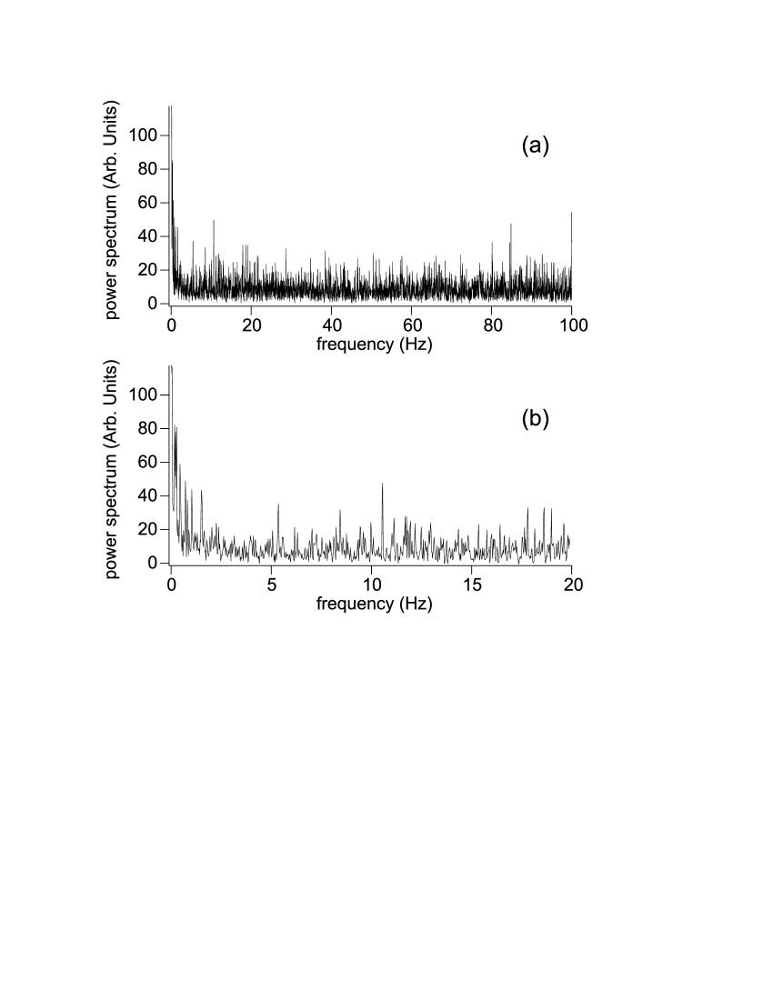
Figure 4: Power spectra corresponding to the behavior illustrated in fig. 3. In (a) CM location, and in (b) cloud population. The scales are linear.

In some situations corresponding to given ranges of parameters nousprl , the ${\bf r}$ dynamics is altered by the appearance of spontaneous large amplitude oscillation-like bursts. As illustrated in fig. 5, the signal inside the bursts is not periodic, although it is clearly dominated by a given frequency. These bursts are relatively scarce, and the global shape of the signal remains that of Fig. 3. The bursts appear in fact as the most spectacular consequence of a deeper change of the dynamics, which is the appearance of a second characteristic time. This appears clearly in the spectrum of $r$ (Fig. 6a) as a peak centered at a frequency $\nu_{r}$, which depends on the parameter values, but ranges typically between 10 and 100 Hz. The other characteristics of the dynamics are not modified by the existence of bursts. In particular, the spectrum still exhibits the low frequency component below $\nu_{n}$, and the bursts do not appear on the $n$ behavior (Fig. 5b and 6b). The low frequency component dynamics of $r$ and the dynamics of $n$ remain correlated. This behavior will be referred in the following as S_H instabilities.

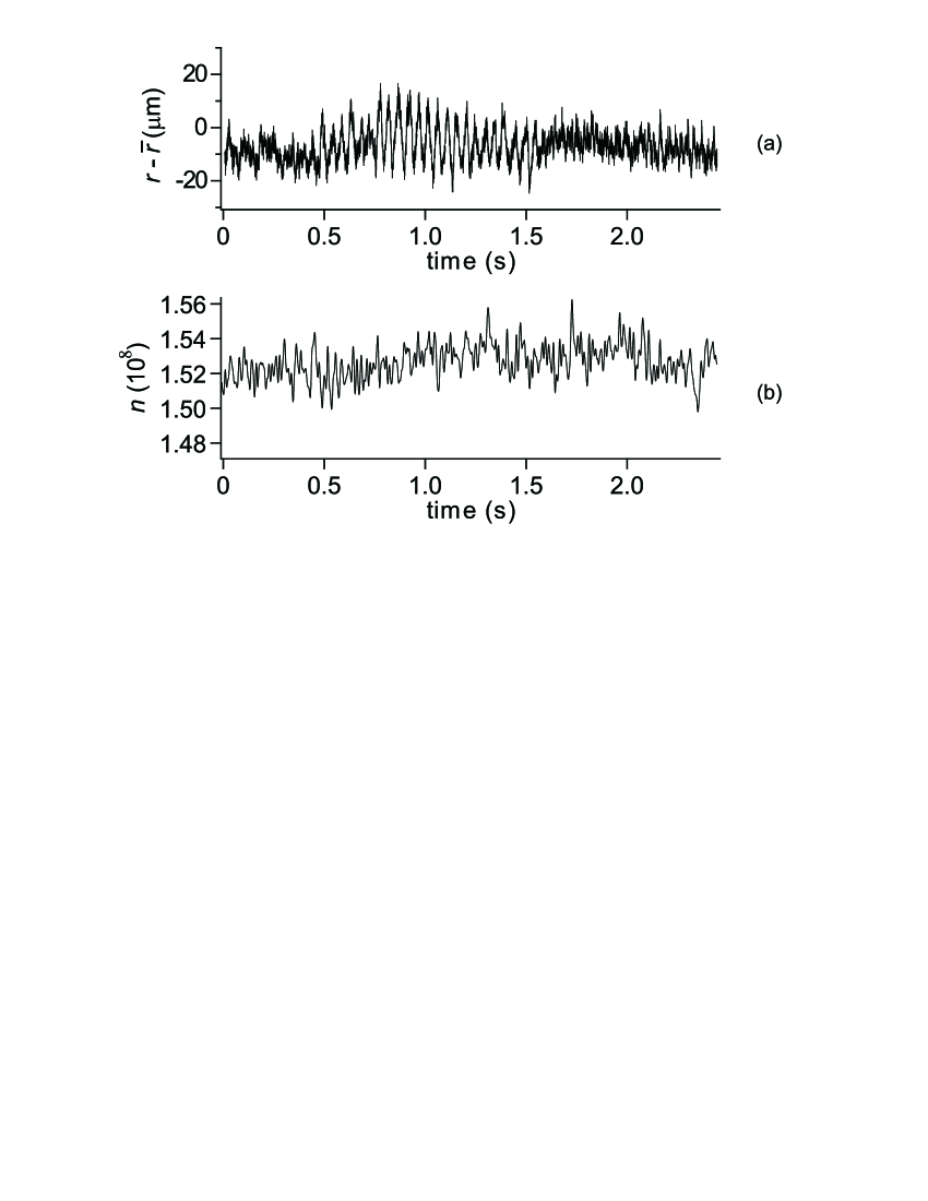
Figure 5: Experimental record of the time evolution of a component of the CM location of the atomic cloud in the case of the S behavior. Experimental parameters correspond to the default set given in Table 1, with $\Delta_{0}=-1.5$. The mean cloud population is $1.5\times 10^{8}$ atoms and the cloud size is 1 mm.

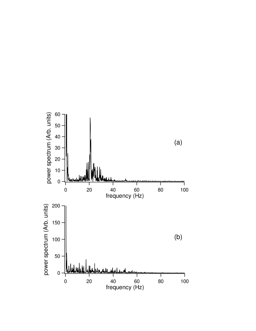
Figure 6: Power spectra corresponding to the behavior illustrated in fig. 5. In (a) CM location, and in (b) cloud population. The scales are linear.

When the trap beam intensity $I_{1}$ is increased, S instabilities still exist, but they are progressively superseded by C instabilities. These instabilities differ drastically from S onesInstDet : they can be either periodic or erratic, but in both cases, they are cyclic, and the motion amplitude is much larger. However, as for S instabilities, C instabilities exist in a limited range of $\Delta_{0}$, which value depends on the other parameters. But it is systematically between $\Delta_{0}=-3$ and resonance, and the maximum detuning range is of the order of $1$.

As $I_{1}$ is increased, the disappearance of S instabilities occurs progressively, in favor of C instabilities. For intermediate values of $I_{1}$, both types of instabilities exist. Their typical distribution versus $\Delta_{0}$ is illustrated in Fig. 7: far from resonance, the cloud is stable; as the resonance is approached, S instabilities appear for a detuning $\Delta_{0}=\Delta_{1}$. Then C instabilities appear in $\Delta_{2}>\Delta_{1}$. If the detuning is still increased, C instabilities disappear in $\Delta_{3}$ at the benefit of a stable behavior. Finally, the cloud vanishes in $\Delta_{4}$. As $I_{1}$ is increased, the width $\delta_{12}=\Delta_{2}-\Delta_{1}$ decreases in favor of the interval $\delta_{23}=\Delta_{3}-\Delta_{2}$, while the total unstable interval $\delta_{13}=\Delta_{3}-\Delta_{1}$ remains more or less constant. When C instabilities merge for $I_{1}=4I_{S}$, they appear on a narrow interval $\delta_{23}\gtrsim 0$. This interval increases rapidly until $I_{1}=7.5I_{S}$ and $\delta_{23}=0.8$. For $I_{1}>7.5I_{S}$, $\delta_{23}$ increases more slowly, to reach the value of $\delta_{23}=1$ in $I_{1}=20I_{S}$, where S instabilities have completely disappeared.

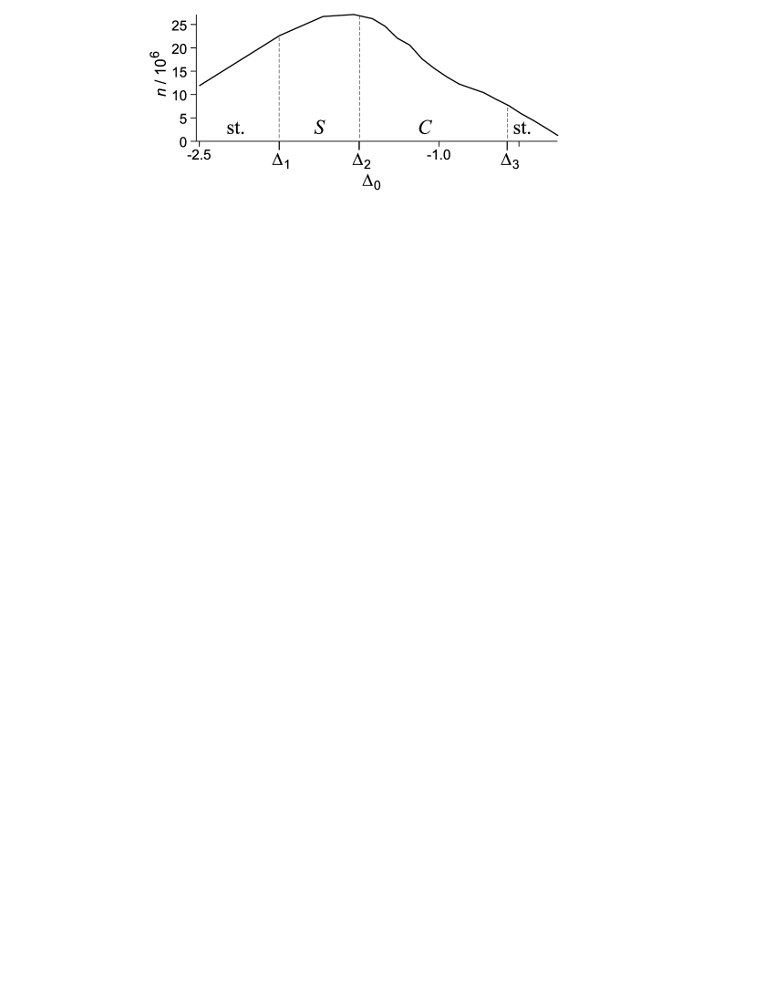
Figure 7: This figure illustrates the evolution of the behavior as a function of the detuning for $I_{1}=6.8$ and $I_{rep}=1.5$ mW/cm². The full line reports the population, while the dashed lines separate the domain of different behaviors: st. stands for stable, S for S instabilities and C for C instabilities.

To conclude this section, let us summarize the main properties of the instabilities: they appear to be stochastic at a time scale larger than 0.5 s. They may exhibit a second dynamical component with time scale smaller than $10^{-2}$ s and acting only on ${\bf r}$. The low frequency component corresponds to a CM motion along the first bisector of the three forward beams. Finally, they appear only in a limited range of the parameters, suggesting a nonlinear origin of the instabilities. This last point was also suggested by different tests showing that beam phase fluctuations are not at the origin of instabilities nousprl .

4 Model

To understand the dynamics observed in the experiments, we build a phenomenological model taking into account the shadow effect. The aim here is not to model as finely as possible the experimental system, but on the contrary to make a model as simple as possible, enlightening the fundamental mechanisms leading to the instabilities.

The model that we used here has already been described in InstDet . It is based on the shadow effect induced by the intensity gradients produced by the absorption of the trapping laser beams in the cloud shadow ; dalibard . The shadow effect generates a force compressing the cloud. In the case where the counter-propagating beams result from the reflection of the three forward beams, this compression is accompanied by a displacement of the CM along the first bisector of the three forward beams: indeed, the backward beams are less intense than the forward ones because of the absorption in the cloud, and so the latter literally push the cloud off its equilibrium location. The main role of the shadow effect in the instabilities is suggested in the experiments (i) by the observed correlation between the $n$ and slow CM dynamics and (ii) by the fact that the slow dynamical component of $r$ displaces the cloud along the first bisector of the three forward beams. The fundamental role of the shadow effect in coupling the population and the CM position of cold atom clouds was already reported in bistab . In that experiment, bistability in the population dynamics was observed by perturbing the atomic cloud with a highly-focalized laser beam, and shadow effect is shown to be the dominant nonlinearity.

We built a 1D model taking into account the shadow effect in a MOT where counter-propagating beams result from the reflection of the three forward beams. As we are interested here in the collective motion, we use as variables the location $z$ of the center of mass of the cloud along the unique axis $z$ of the system, and the number of atoms $n$ inside the cloud. The origin of $z$ coincides with the “trap center”, that is, the zero of the magnetic field. Thus, the motion of $z$ may be described by the equation:

$$\frac{d^{2}z}{dt^{2}}=\frac{1}{M}F_{T}$$ (1)

where $M$ is the mass of the cloud and $F_{T}$ the global force exerted on the atoms by the two counterpropagating beams. To evaluate $F_{T}$, we assume a multiple scattering regime, i.e. a constant atomic density $\rho$ in the cloud. The atoms are distributed between $z_{\min}$ and $z_{\max}$, and the quantity $\Delta z=z_{\max}-z_{\min}$ is the longitudinal size of the cloud. We introduce a constant cross section $S$, allowing us to connect $\Delta z$ to $n$:

$$n=\rho S\Delta z$$ (2)

The repulsive force induced by the multiple scattering is an internal force, and thus does not affect directly the center of mass motion. It is also the case for the attractive force induced by the shadow effect, which acts on $F_{T}$ only through the asymmetry between the forward and backward beams. The forward beam is polarized $\sigma_{+}$ and has an input intensity $I_{1}$. After the crossing of the cloud, its output intensity is $I_{2}$. This is also the input intensity of the backward beam, which is polarized $\sigma_{-}$. After the crossing of the atomic cloud, the output intensity of the backward beam is $I_{3}$. We have obviously $I_{1}>I_{2}>I_{3}$. $F_{T}$ is proportional to the number of photons absorbed per unit time, i.e. $S(I_{1}-I_{2})/\hbar\omega_{L}$ for the forward beam and $S(I_{2}-I_{3})/\hbar\omega_{L}$ for the backward beam ($\hbar\omega_{L}$ is the energy of one photon, $\omega_{L}$ being the laser angular frequency). $F_{T}$ is obtained by multiplying the difference between both quantities by $\hbar k_{L}$

$$F_{T}=\frac{S}{c}(I_{1}-2I_{2}+I_{3})$$ (3)

To evaluate $I_{2}$ and $I_{3}$, we need to solve the propagation equation of light inside the cloud. To simplify the calculations, we choose to model a $F_{g}=0\rightarrow F_{e}=1$ transition: this is the simplest one leading to a magneto-Doppler effect. This choice does not allow us to reproduce the sub-Doppler effects, neither the photon redistribution between the two waves, but as shown in InstDet , it allows us to explain most of the experimental behaviors.

The $z$ axis is chosen as quantification axis, and we introduce the ground state $|g\rangle$ and the three Zeeman sub-levels of the excited state $|e_{0}\rangle$ et $|e_{\pm}\rangle$. Because of the kinetic momentum conservation, $|e_{0}\rangle$ is not coupled to the light field, and thus, the model is reduced to a three level system, $\{|g\rangle,|e_{-}\rangle,|e_{+}\rangle\}$. The interaction with light is governed by the Rabi frequency $\Omega_{\pm}$ and the effective detunings $\Delta_{\pm}$, taking into account the Doppler et Zeeman variations:

$$\Delta_{\pm}=\frac{1}{\Gamma}(\Delta_{0}\mp kv\mp\omega_{B}^{\prime}z)=\frac{1}{\Gamma}(\Delta_{0}\pm 2\delta)$$ (4)

where $k$ is the wave vector of light and $\omega_{B}^{\prime}$ the Zeeman shift, measured in angular frequency by unit of length. The value of the atomic variables is given by the stationary solution of the optical Bloch equations for the density matrix $\sigma$:

$$\dot{\sigma}=\frac{1}{i\hbar}[H\;,\sigma\;]+\dot{\sigma}_{relax}$$ (5)

The hamiltonian $H$ of coupling with light may be written as a function of $\Delta_{\pm}$ and $\Omega_{\pm}$ in the $\{|g\rangle,|e_{-}\rangle,|e_{+}\rangle\}$ basis:

$$H=\hbar\left(\begin{array}[]{ccc}0&\Omega_{-}/2&\Omega_{+}/2\\ \Omega_{-}^{\ast}/2&-\Delta_{-}&0\\ \Omega_{+}^{\ast}/2&0&-\Delta_{+}\end{array}\right)$$ (6)

The relaxation rates $\dot{\sigma}_{relax}$ are different for the excited states, the optical coherences and the ground state:

$$(\dot{\sigma_{ee}})_{relax} = -\Gamma\sigma_{ee}$$ (7a)

$$(\dot{\sigma_{eg}})_{relax} = -\frac{\Gamma}{2}\sigma_{eg}$$ (7b)

$$(\dot{\sigma_{gg}})_{relax} = -\Gamma(\sigma_{++}+\sigma_{--})$$ (7c)

The time scale of the internal variables is $$\Gamma^{-1} z v \Pi_{\pm}=\sigma_{\pm\pm} \Pi_{\pm}$$, and so is much shorter than that of the external variables and . Thus the stationary solution of Eq. (5) can be used. The solution for the populations of the excited states can be obtained analytically. On the other hand, as the redistribution of photons between the beams is forbidden, is directly proportional to the absorption rate of the beams, and the intensity gradient can be written:

$$\frac{dI_{\pm}}{dz}=\mp\Gamma\hbar\omega_{L}\rho\Pi_{\pm}$$ (8)

By injecting the analytical solution of $\Pi_{\pm}$ in this equation, we obtain the following equations of propagation:

$$\frac{dI_{+}}{dz} = -\Gamma\hbar\omega\rho\frac{\theta\omega_{+}\omega_{-}+C_{-}\omega_{+}}{1-A_{+}\omega_{+}-A_{-}\omega_{-}+3\theta\omega_{+}\omega_{-}}$$ (9a)

$$\frac{dI_{-}}{dz} = \Gamma\hbar\omega\rho\frac{\theta\omega_{+}\omega_{-}+C_{+}\omega_{-}}{1-A_{+}\omega_{+}-A_{-}\omega_{-}+3\theta\omega_{+}\omega_{-}}$$ (9b)

where:

$$\omega_{\pm} = -\frac{I_{\pm}}{2\gamma}$$ (10a)

$$\gamma = \frac{1}{4}\left[\left(\alpha+\beta_{+}+\beta_{-}\right)^{2}+\left(\frac{\beta_{+}-\beta_{-}}{\Delta_{0}}\right)^{2}\right]$$ (10b)

$$\alpha = \frac{1+2\mu}{4}+\Delta_{+}\Delta_{-}+\frac{\delta^{2}}{2}\left(\mu-1\right)$$ (10c)

$$\beta_{\pm} = \frac{\alpha}{2}\pm\left(\Delta_{0}\pm\delta\right)\left(\frac{\delta}{2}+\Delta_{0}\left(\mu_{+}-\mu_{-}\right)\right)$$ (10d)

$$\mu_{\pm} = \frac{I_{\pm}}{4\left(1+\delta^{2}\right)}$$ (10e)

$$\mu = \mu_{+}+\mu_{-}$$ (10f)

$$\theta = \beta_{+}\beta_{-}+\alpha\left(\beta_{+}\mu_{+}+\beta_{-}\mu_{-}\right)$$ (10g)

$$A_{\pm} = 2\beta_{\mp}+\alpha\left(2\mu_{\pm}-\mu_{\mp}\right)$$ (10h)

$$C_{\pm} = -\beta_{\pm}\pm\alpha\left(\mu_{+}-\mu_{-}\right)$$ (10i)

These equations appear as the ratio of two polynomials of high order, and an intuitive interpretation of this result is difficult. However, a numerical resolution of these equations leads to a rigorous evaluation of $$F_{T}$$.

The cloud population dynamics is modeled by a “feed-loss” rate equation feedloss :

$$\frac{dn}{dt}=B\left(n_{e}-n\right)$$ (11)

where we have introduce the population relaxation $B$ and the atom number in the cloud at equilibrium $n_{e}$, which is linked to the loading rate $L$ by $L=Bn_{e}$. $n_{e}$ is assumed to depend on the CM location, to take into account the losses variation when the cloud moves from the trap center. We do not know the exact form of this dependence, because this variation may have several origins. However, we can suppose that the main contribution comes from the transverse distribution of the trap laser beam, which is gaussian. For sake of simplicity, we keep only the first terms from its Taylor’s series, i.e. the quadratic term. In fact, we checked that the exact dependence of $n_{e}$ does not change drastically the results given below. So we write:

$$n_{e}=n_{0}\left[1-\left(\frac{z}{z_{0}}\right)^{2}\right]$$ (12)

where $n_{0}$ is the equilibrium cloud population at the trap center and $z_{0}$ a characteristic length. Atoms in $\left|z\right|>\left|z_{0}\right|$ are considered as lost: this is taken into consideration when $n$ is deduced from Eq. 2.

Finally, we introduce the reduced variables $Z=z/z_{0}$, $V=v/v_{r}$ and $N=n/n_{0}$, where $v_{r}$ is the recoil velocity ($v_{r}=\hbar k/m$), and we obtain the following autonomous system of equations:

$$\frac{dZ}{dt} = V\frac{v_{r}}{z_{0}}$$ (13a)

$$\frac{dV}{dt} = \frac{1}{Mv_{r}}F_{T}$$ (13b)

$$\frac{dN}{dt} = B\left(1-Z^{2}-N\right)$$ (13c)

Most of the theoretical parameters are the exact counterpart of the experimental parameters, as e.g. the magnetic field gradient or the beam intensities. In this case, we used in the model the same values as those of Table 1. It is not the case for all parameters, either because of the simplicity of the model or because they cannot be measured easily in the experiment. For example, $n_{0}$ has not a simple experimental counterpart, but depends on several experimental parameters, as e.g. the repumping laser intensity or the vapor pressure in the cell. For this reason, a large interval of $n_{0}$ values has been used for the simulations (Table 2). The density $\rho$ and the cross sectional area $S$, which play the same role, have a meaning only in the context of a 1D model, while they correspond to variables in the experiments. They are fixed in the simulations at experimental averaged values, and they have been varied on a wide range to check that their value is not critical. Finally, the parameter $z_{0}$ has not exact experimental counterpart, as it is linked to both the trap beam waist and intensities. Indeed, the relevant size for the atoms is not the beam waist, corresponding to an intensity decreased by a ratio $e^{-2}$ as compared to the center of the beam, but rather the location where the local beam intensity decreases under $I_{S}$. This value is much larger than $w_{0}$ for intense beams.

Table 2: Parameters used in the numerical simulations. The range corresponds to the interval explored numerically, while the different sets refer to most of the results presented in this paper.

	range	set #1	set #2
$G$ (Gcm-1)	$14$	$14$	$14$
$B$ (s-1)	$3\leq B\leq 30$	$3$	$3$
$I_{1}$	$2\leq I_{1}\leq 30$	25	10
$\rho$ (cm-3)	$10^{10}\leq\rho\leq 3\times 10^{10}$	$2\times 10^{10}$	$2\times 10^{10}$
$S$ (m2)	$10^{-6}\leq S\leq 3\times 10^{-6}$	$10^{-6}$	$10^{-6}$
$z_{0}$ (m)	$10^{-2}\leq z_{0}\leq 3\times 10^{-1}$	$3\times 10^{-2}$	$3\times 10^{-2}$
$n_{0}$	$10^{7}\leq n_{0}\leq 10^{9}$	$10^{8}$	$2\times 10^{7}$
$\Delta_{0}$	$5\leq\Delta_{0}\leq 0$	$-1.5$	$-0.23$

In order to check if the model can be more simplified, we tried to reproduce the unstable dynamics of the cloud with the first terms of the Taylor’s series of Eqs. (9a) et (9b), but we needed to keep several orders and did not obtain simpler equations. Another possible approximation concerns the different terms appearing in $\Delta_{\pm}$, in Eq. 4. Using the values given in table II, one sees easily that the $\Delta_{0}$ term and the Zeeman shift are of the same order of magnitude, while the Doppler shift goes to zero at equilibrium, but can be the largest term out of equilibrium. In these conditions, no approximation is possible. Therefore, we use the equations (13) in the calculations.

To perform the comparison between the experiments and the present model, we need to study the behavior of the system when noise is added. Noise can be added in Eqs 13 on any parameter, and as we were not able in our experiments to identify clearly the main source of noise, we tried theoretically several parameters, as the beam intensity $I_{1}$ or the equilibrium population $n_{0}$. In this case, the stochastic model corresponds to Eqs 13 where the parameter $I_{1}$ (resp. $n_{0}$) is replaced by $\left(1+\zeta\right)I_{1}$ (resp. $\left(1+\zeta\right)n_{0}$), where $\zeta(t)$ is the noise component. We also simulated several types of noise: gaussian white noise, but also colored noise with different distributions of the frequencies. All configurations give identical results: on the one hand, the choice of the noisy parameter is not critical; on the other hand, the spectrum of noise does not alter the response spectrum, except obviously that it depends on the relative weight of the different frequencies in the noise. Thus, for sake of clarity, all the results reported in the following have been obtained by applying with gaussian white noise on $I_{1}$.

5 Stationary solutions

In the previous section, we built a relatively simple model where the cloud is described by a set of three equations that do not depend explicitly on the time. Such a system is known to be able to exhibit a complex dynamics, including chaos, which could explain the experimental instabilities. To know if such a complex dynamics occur in our conditions, the first step is to evaluate the stability of the stationary solutions. The stationary solutions ($V_{s}$, $Z_{s}$, $N_{s}$) of the model with the shadow effect are easily deduced from Eq.13 when the left side is put to zero. Eq. 13a gives immediately $V_{s}=0$. From Eq. 13c, one finds that the stationary solutions $Z_{s}$ of the CM location and $N_{s}$ of the population are linked by the simple expression:

$$N_{s}=1-Z_{s}^{2}$$ (14)

Therefore, the discussion is reduced to the analysis of $Z_{s}$. $Z_{s}$ is the solution of $F_{T}=0$ in Eqs 13b. This equation can be resolved numerically: its global shape is illustrated in Fig. 8, where it is plotted as a function of $\Delta_{0}$ and $n_{0}$.

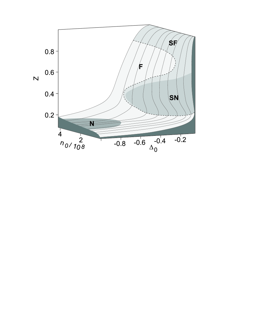
Figure 8: Stationary solutions of equations 13 versus $n_{0}$ and $\Delta_{0}$. The figure represents $Z_{s}$. Other parameters correspond to the set #1 given in table 2. The definition of the N, F, SN and SF zones (each corresponding to different level of greys) is given in the text.

A first characteristic of the $Z_{s}$ diagram is that $Z_{s}$ goes to $1$ (i.e. $N_{s}$ goes to zero) at resonance. This vanishing of the cloud, also observed in the experiments, is a well-known consequence of the inefficiency of the Doppler cooling close to resonance. It is here enhanced by the shadow effect and the displacement of the cloud. The disappearance occurs suddenly for small $n_{0}$, and becomes softer as $n_{0}$ increases. An interesting point is that for small $n_{0}$, the abrupt increase of $Z_{s}$ is linked to a very narrow bistable cycle. As $n_{0}$ is increased, the bistable cycle shifts towards smaller $Z_{s}$ and smaller $\Delta_{0}$, and the vanishing of $Z_{s}$ becomes progressive.

The main characteristic of the $Z_{s}$ diagram is the presence of several abrupt slope changes in the stationary solutions, leading to a fold in the parameter space. The shape of the fold depends on the parameters, in particular on $n_{0}$. Fig. 9 shows four examples corresponding to situations leading to basically different atomic dynamics. For $n_{0}=0.5\times 10^{8}$ (fig. 9a), $Z_{s}$ increases smoothly with $\Delta_{0}$ (i.e. $N_{s}$ decreases slowly). The vanishing of the cloud through a narrow bistable cycle is not visible on the graph, as it occurs closer from resonance. As $n_{0}$ increases, the bistable cycle appears for smaller $Z_{s}$ (and thus larger $N_{s}$), and becomes physically significant. Fig. 9b shows $Z_{s}$ for $n_{0}$ $=2.5\times 10^{8}$ and a bistable cycle for $-0.3\lesssim\Delta_{0}\lesssim-0.25$. If $n_{0}$ is further increased, the bistable cycle disappears, but it remains a fold corresponding to two abrupt slope changes of $Z_{s}$ versus $\Delta_{0}$ (fig. 9c, $n_{0}$ $=3.4\times 10^{8}$). If $n_{0}$ is still increased, the fold remains, but it becomes smoother (Fig. 9d for $n_{0}=$ $4\times 10^{8}$).

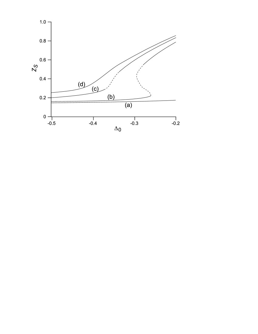
Figure 9: Evolution as a function of the detuning of the stationary solution $Z_{s}$ of equations 13. The full (resp. dashed) line corresponds to a stable (resp. unstable) solution. In (a), $n_{0}=0.5\times 10^{8}$; in (b) $n_{0}=2.5\times 10^{8}$; in (c), $n_{0}=3.4\times 10^{8}$; in (d), $n_{0}=4\times 10^{8}$ Other parameters correspond to the set #1 of Table 2

The dynamics of the cloud is determined by the stability of these stationary solutions. In particular, if no stationary solutions are stable, complex dynamics could be obtained. The stability of the above stationary solutions is evaluated through a linear stability analysis, which associates to each stationary solution its three eigenvalues, corresponding to the stability following its three eigendirections in the 3D phase space of our model. The real part of the eigenvalue, corresponding to a damping rate, determines the stability (stable if negative). The imaginary part, when different from zero, is associated to an angular eigenfrequency, also called relaxation frequency, which play a main role in the dynamics. A pleasant – and simple – way to describe the stationary solutions is to use their phase space representation, where each stationary solution corresponds to a fixed point with its properties depending on its eigenvalues. Let us remember that the standard terminology distinguishes the stable node (all eigenvalues real and negative), the stable focus (all real parts negative, two eigenvalues complex conjugate), the saddle node (all eigenvalues real, at least one positive) and the saddle focus (at least one real part positive, two eigenvalues complex conjugate). For sake of simplicity, this terminology will be used in the following.

The set of points of vertical tangency in $Z_{s}$ determines a line which delimits the unstable stationary solution of the medium branch of the bistability cycle. Linear stability analysis shows that the fixed point in that area is a saddle-node with real eigenvalues, two being positive and one negative. But the unstable stationary solutions extend beyond this area. In particular, the stationary solutions can also be unstable on a part of the upper branch of the bistable cycle, and even outside the bistable cycle, when the stationary solution is unique. This is illustrated on fig. 8 where the nature of the stationary solution is indicated by a level of gray and a code. In the SN zone, the fixed point associated with the stationary solution is a saddle node, i.e. the stationary solution is unstable, and its three eigenvalues are real, two being positive. In the SF zone, the fixed point is a saddle focus, i.e. the stationary solution is unstable, and two of its eigenvalues are complex with a positive real part, and the third one is real negative. In the F zone, the fixed point is a stable focus, i.e. the stationary solution is stable, and two of its eigenvalues are complex with a negative real part, the third one is real negative. Finally, in the N zone, the fixed point is a stable node, i.e. the stationary solution is stable and all eigenvalues are real negative. The dashed line indicates the location of the bifurcation, i.e. the transition from stable to unstable stationary solutions. In most cases, it occurs from stable focus to saddle focus, through a super-critical Hopf bifurcation.

As the detuning is varied, four typical situations may occur, already illustrated in Fig. 9. For small $n_{0}$ (Fig. 9a), $Z_{s}$ is always stable, and its dependence versus $\Delta_{0}$ is almost flat (except very close from resonance): we expect a stationary cloud slightly moving with the detuning. In the bistability area (Fig. 9b), the central branch of the bistability cycle is unstable, as usual in such a situation, but the upper branch is also partly unstable, reducing drastically the parameter range where the system is effectively bistable. However, a narrow bistable zone should be observed. As $n_{0}$ is still increased, only one stationary solution remains (Figs 9c), which is unstable on the fold.

Finally, for large $n_{0}$ (Fig. 9d), the solution is always stable (F zone), except very close from resonance. Thus we expect to observe a stationary cloud moving with $\Delta_{0}$. However, because of the fold, this moving is non linear, and on the fold, for $-0.45<$ $\Delta_{0}<-0.35$, $Z_{S}$ is more sensitive to the $\Delta_{0}$ value, because the slope here is larger. On the other hand, a closer look to the eigenvalues (Fig. 10) shows that at the level of the fold, the real part $\lambda$ of the complex eigenvalues $\lambda\pm i\omega$ is close to zero, while the eigenfrequency crosses a minimum. This is more evident on Fig. 11, where the same situation is illustrated for a different set of parameters. The vanishing damping rate $\left|\lambda\right|$ associated to an increased sensitivity to the parameter values means that a small perturbation will cause a large undamped reaction of the system, with relaxation oscillations at a frequency $\omega$ crossing a minimum while $\Delta_{0}$ is varied on the fold. In the fold inflection point, where the slope is maximum, the eigenfrequency and damping rate are minimum: the effects of perturbations is expected to be maximum at this point. Note that the evolution of $\lambda$ and $\omega$ around the inflection point is asymmetric: the damping rate and relaxation frequency increase rapidly for detunings smaller than the inflection point, while they remain of the same order of magnitude on the other side. This asymmetry is expected to have consequences on the dynamics.

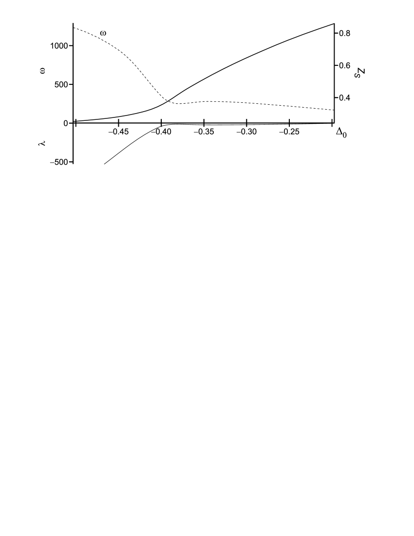
Figure 10: Evolution as a function of the detuning of the stationary solution $Z_{S}$ and its eigenvalues, for the parameters of Fig. 9d. The stationary solution is given through the full bold line in the upper side of the figure. The dashed line noted $\omega$ represents the imaginary part of the complex eigenvalues, while the full line corresponds to their real part $\lambda$. The third eigenvalue is always real negative, almost constant and everywhere larger than $\lambda$. It cannot be distinguished from the zero axis at the scale of the figure.

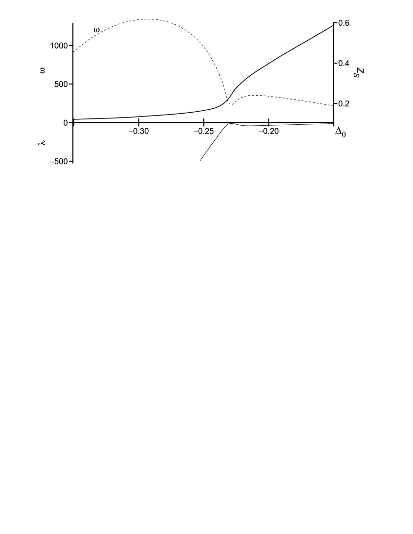
Figure 11: Same as Fig. 10 for parameter set #2 of Table 2. For sake of clarity, the evolution of $\lambda$ has been truncated for small detunings, where it becomes almost linear, reaching e.g. the value of $\lambda=-1500$ for $\Delta_{0}=-0.3$.

Deterministic instabilities are expected to occur for parameters where all stationary solutions are unstable, i.e. in the SF monostable zoneInstDet . In all other areas, the stationary solutions are stable, and therefore, deterministic instabilities cannot occur. However, the presence of the fold and the proximity of a Hopf bifurcation generate a type of stochastic behavior similar to instabilitiesnousprl .

Indeed, on the one hand, the proximity of a Hopf bifurcation is known to favor the appearance of coherence resonanceSRlike , as discussed in nousprl . Let us recall that coherence resonance is the counterpart of stochastic resonance in autonomous systemsSRRevue . Stochastic resonance appears in some forced systems: it may be seen as an amplification by noise of the system response to a forcing. In other terms, the signal to noise ratio of the output periodic signal resulting from the modulation exhibits a maximum when the noise amplitude increases. In stable autonomous systems, the behavior is not periodic, but a phenomenon similar to stochastic resonance can lead to an amplification of an internal resonance: it is the internal stochastic resonance, or coherent resonance CohRes ; CohResPrecursor . Coherent resonance is also known to generate noise induced coherent oscillations, which explain some of our experimental observations, as shown in nousprl .

On the other hand, as shown above, the particular configuration of the eigenvalues on the stable fold makes the system very sensitive to small perturbations, i.e. to noise, and thus we expect a large increasing of the response to noise on the fold. The resulting behavior looks like instabilities, whereas it is simply noise amplification. The behavior obtained on the stable fold when noise is taken into account is detailed in the next section.

6 The stable fold: stochastic instabilities

In InstDet , it has been shown that the model is able to reproduce the C instabilities, in the monostable SF zone. On the contrary, S instabilities do not appear in this situation. In fact, it has been shown in nousprl that S instabilities are not instabilities in the usual significance, but the result of the amplification of the system intrinsic noise, and thus it is necessary to add noise in the simulations to observe S instabilities. This dynamics could appear when the stationary solution of the MOT is not stable, but would be difficult to analyze, because in this case the resulting dynamics would be the superimposition of the deterministic instability with the stochastic motion, the latter being masked by the former. For this reason, the present section is devoted to the study of the influence of noise on the stable stationary solutions of the model, in particular in the vicinity of the fold. As the model here is slightly different from that used in nousprl , we could expect different results from those obtained in nousprl . It is shown in the following that the modifications introduced in the model do not alter the previous conclusions, i.e. that S instabilities are produced by noise amplification on the fold.

To evaluate the response of the system to noise in the vicinity of the fold, we have plotted the amplitude of the motion perturbed by noise, versus the detuning, across the fold (Fig. 12). The amplitude of the motion is measured through the standard deviation $\sigma$ of $Z$. Fig. 12 has been obtained for a gaussian white noise applied on $I_{1}$ with an amplitude of $10^{-3}$, in a situation where the stationary solutions are stable on the fold. Noise amplification appears clearly on the fold, and mimics instabilities, as in the experiments (Fig. 2). The maximum of the motion amplitude, obtained for $\Delta_{0}=-0.23$, corresponds to a standard deviation of $1.1\times 10^{-3}$, i.e. $33$ $\mu$m, in good agreement with the experimental value. By comparison, the motion amplitude is $0.036$ for $\Delta_{0}=-3$, i.e. the effect of noise is $30$ times larger on the fold than in $\Delta_{0}=-3$. Note that, as similar motion amplitudes are obtained in the experiment and in the model for a noise level $\zeta=10^{-3}$, this gives us in return an evaluation of the experimental noise level.

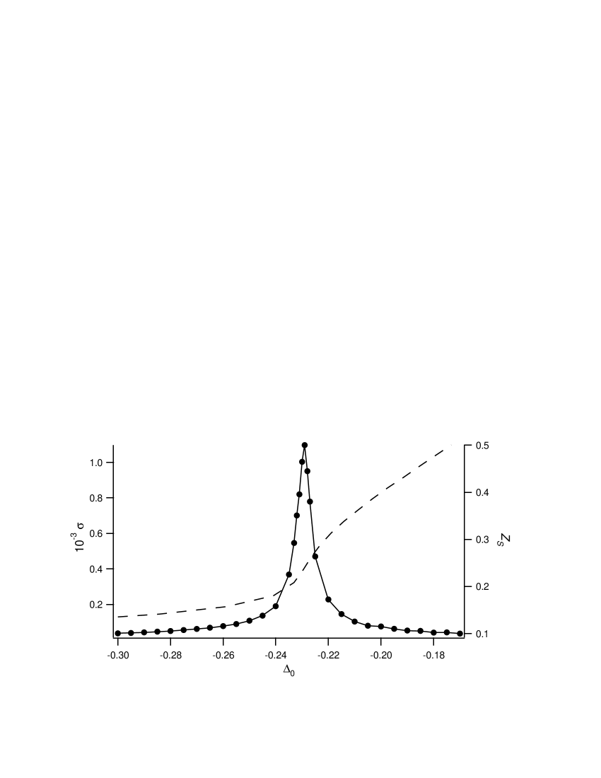
Figure 12: Evolution of the signal standard deviation $\sigma$ (full line) and of the cloud location stationary solution $Z_{S}$ (dashed line) as a function of the detuning $\Delta_{0}$. White noise is applied to $I_{1}$ with $\zeta=10^{-3}$. Other parameters correspond to the set #2 of Tab. 2.

Thus, as for the model developed in nousprl , the fold plays the role of a noise amplifier, leading to an unstable cloud over a limited range of the parameters. The maximum of the motion amplitude appears at the fold inflection point. The amplitude decreases progressively and quasi symmetrically on each side of this point, in spite of the asymmetry of the eigenvalues discussed in the previous section. The range where the instabilities can be observed, appears to be of the order of the “width” of the fold, that we could define as the interval between the two abrupt slope changes delimiting the fold (a more precise definition could be given, but is not useful for the following). In the case discussed here, the range in detuning is 0.02, i.e. much smaller than the experimental range, which was typically of the order of 1. However, the width of the slope is very dependent on the MOT parameters: for example, on Fig. 10, where $I_{1}$ and $n_{0}$ are different, the fold is more than twice larger than in the present case. Thus there is no doubt that it is possible to find a parameter set giving a correct fold width. However, because of the extreme simplicity of the model as compared to the experiments, such a search has no meaning: the aim here is just to show that very few ingredients, including the shadow effect and the noise, are able to reproduce the global experimental behavior. We have now demonstrated that the noise response can effectively have the appearance of instabilities for some parameters. We will now examine in detail the resulting dynamics, and compare it to the experimental observations.

Fig. 13 shows the time evolution of $Z$ and $N$ in $\Delta_{0}=-0.23$, where the amplification is maximum. The signal is of course stochastic, but several differences appear, on the one hand between the cloud response and the applied noise, and on the other hand between the $Z$ and $N$ evolutions. Indeed, while the applied noise is white, a frequency dominates in the response, in particular for $Z$. This is clearly visible on the signal, and of course on the spectrum (Fig. 14), where a peak appears at a frequency $\omega_{S}\simeq 38$ Hz. For $N$, while the frequency $\omega_{S}$ still appears, low frequency fluctuations dominates, as it is also shown by the spectrum (Fig. 14). This behavior with two different characteristic times is very similar to the experimental S_H behavior illustrated in the Fig. 6: in both cases, the higher frequency component dominates the motion of the atoms, while the number of atoms in the cloud is mainly driven by the low frequency component.

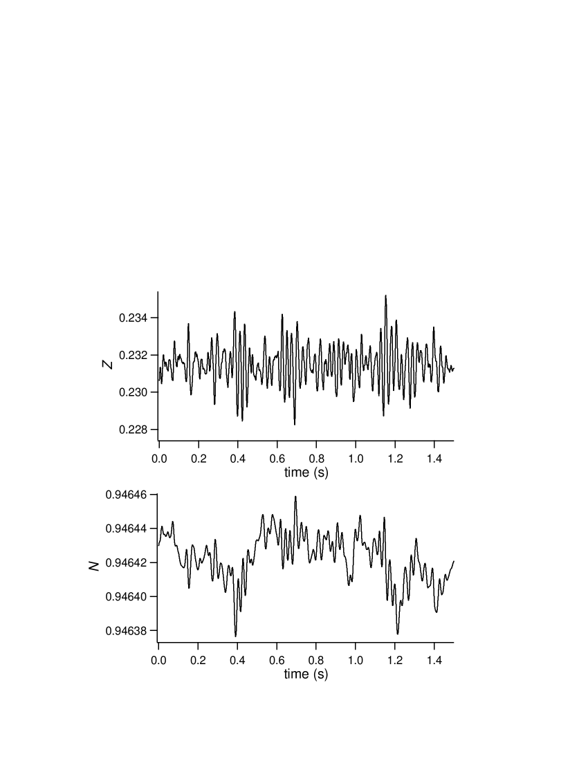
Figure 13: Dynamics obtained by resolving Eqs. (13), with the parameter set #2 and $\Delta_{0}=-0.926$. White noise is applied to $I_{1}$ with $\zeta=10^{-3}$.

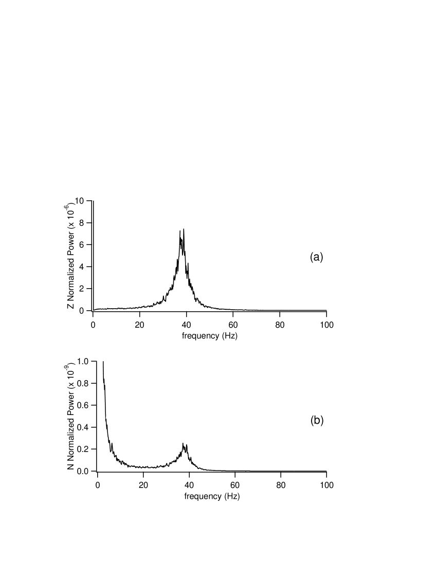
Figure 14: Power spectra obtained by resolving Eqs. 13 with the same parameters as in Fig. 13.

In the experiments, the origin of the higher frequency was not identified, as it does not correspond to a known experimental characteristic frequency. However, we know now that the stable stationary solution on the fold has complex eigenvalues, and thus is associated with a relaxation frequency. As noise is known to be able to excite such non linear resonance eigenfrequenciescelet , it is interesting to compare in the simulations the frequency appearing in the dynamics with the eigenfrequency of the stationary solution. This is illustrated on Fig. 15 for different values of the detuning. The full and dashed lines concern the stationary solutions: they shows the evolution of $\omega$ and $Z_{S}$ versus $\Delta_{0}$. They are a reproduction of Fig. 11, and are recalled just for comparison. The squares give the resonance frequencies of the noisy dynamics. They are obtained by fitting  the calculated spectra of $Z$, as illustrated on Fig. 14a, with a lorentzian function. Similar fits on the $N$ spectra give the same results. Fig. 15 shows that for detunings larger than the fold inflection point, the noisy resonance frequency and the eigenfrequency correspond exactly. This confirms that the frequency appearing in the dynamics is the relaxation frequency appearing in the eigenvalues associated with the stationary solution. Thus “instabilities” appear in fact as a noisy amplification of the relaxation frequency of the MOT, through a phenomenon already observed in many other systems, as e.g. in lasers celet : the small damping rate allows noise to excite the relaxation frequency, altering the frequency distribution of the system response to noise.

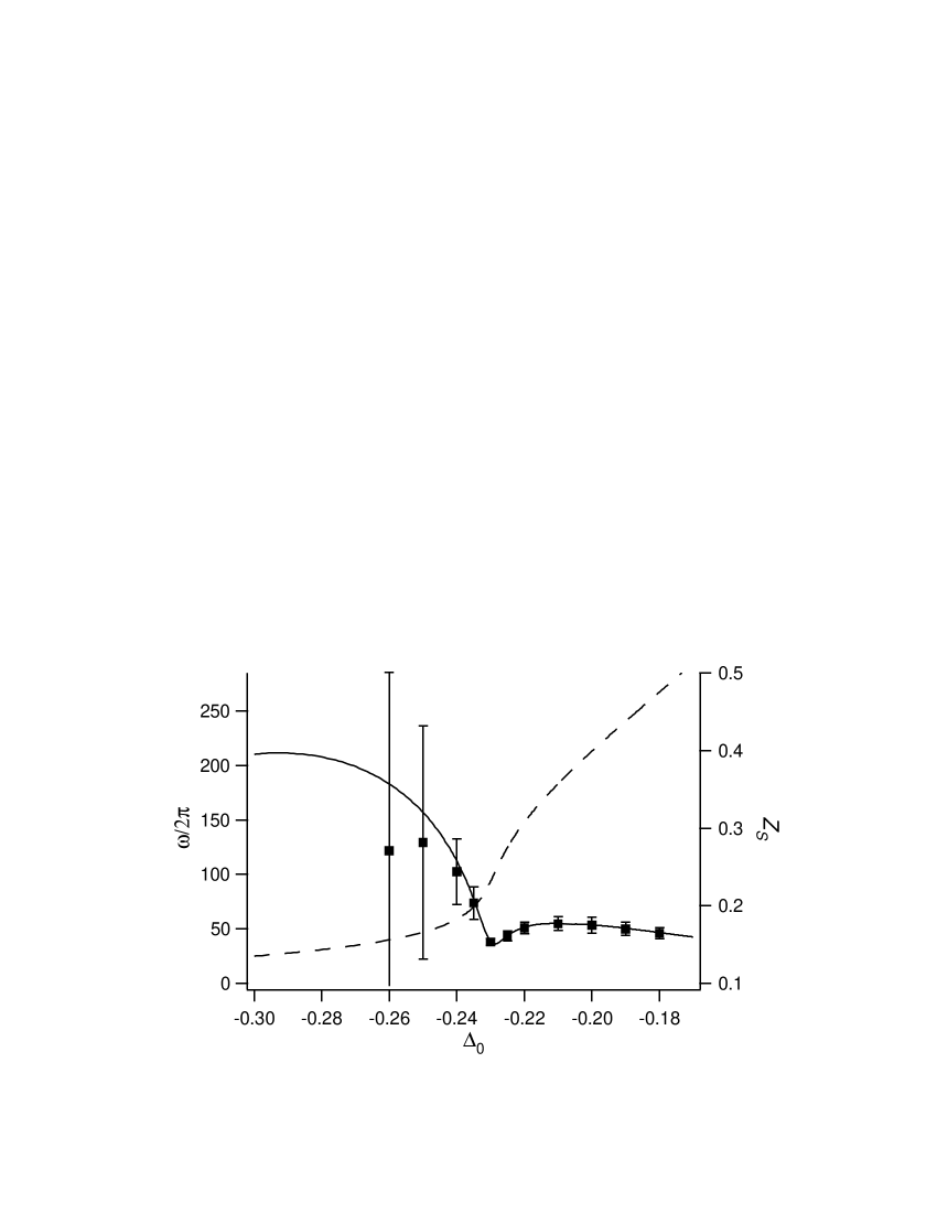
Figure 15: Evolution of the resonance frequencies as a function of the detuning. The full and dashed line recalls the evolution of $\omega$ and $Z_{S}$, already shown on Fig. 11. The squares represent the resonance frequencies appearing in the dynamics, obtained by fitting a lorentzian function on spectra similar to those of fig. 14. The bars give the width of the lorentzian.

For detunings smaller than the fold inflection point, Fig. 15 exhibits differences between the eigenfrequencies and the resonance frequencies. A close look at the dynamics of the cloud shows that the main point is not this difference, but a dramatic broadening of the noise resonance, leading to an indetermination of the resonant frequency. This is illustrated on Fig. 15, where the bars associated with each point have a height of $\Delta\nu$, the width of the lorentzian peak obtained by fitting the $Z$ spectrum. On the inflection point, the resonance is narrow, as it appears on Fig. 14. On the right of the inflection point, the resonance remains narrow, reaching a maximum of $\Delta\nu=14$ Hz in $\Delta_{0}=-0.2$. On the contrary, for detunings smaller than the inflection point, $\Delta\nu$ increases rapidly, reaching already the value $\Delta\nu=30$ Hz in $\Delta_{0}=-0.235$ (the inflection point is in $\Delta_{0}=-0.23$). It is clear on Fig. 15 that the discrepancy between the noise resonance and the relaxation frequencies is linked to the width of the resonance: as the resonance broadens, it also flattens, and the central frequency becomes irrelevant. This is the reason why the resonant frequencies for detunings smaller than $\Delta_{0}=-0.26$ are not reported on the figure.

This asymmetry in the dynamics around the fold inflection point is of course linked to the asymmetry in the eigenvalues associated with the stationary solution. For detunings larger than the inflection point, the damping rate remains small (less than 45 s^-1), and thus the noise excitation of the relaxation oscillations remains efficient. On the contrary, for detunings smaller than the inflection point, the damping rate increases rapidly, decreasing the efficiency of the excitation, and leading to a flat resonance. The consequence on the dynamics is illustrated on Fig. 16, where the power spectra of the $Z$ dynamics are represented for two different values of the detuning, located symmetrically with respect to the inflection point. In (a), for $\Delta_{0}=-0.22$, i.e. for a larger detuning than the inflection point, the resonance, centered on 50 Hz, remains narrow ($\Delta\nu=11$ Hz), and thus significant. In (b), for $\Delta_{0}=-0.24$, i.e. on the other side of the inflection point, the resonance, centered on 100 Hz, is already 60 Hz wide, and also five times lower (note the different vertical scales in (a) and (b)). Such a resonance is no more significant from an experimental point of view: indeed, the experimental dynamics is analyzed from time series with a necessary limited number of points, leading to spectra with a resolution much smaller than in the simulations. It is clear that a resonance as those observed on the left of the inflection point could not be detected in the experiments, and thus one expects that in this situation, experiments deliver non resolved spectra. It was effectively the case for S_L instabilities (Fig. 4), and thus we can conclude that the S_L dynamics observed in the experiments is also explained by the present model.

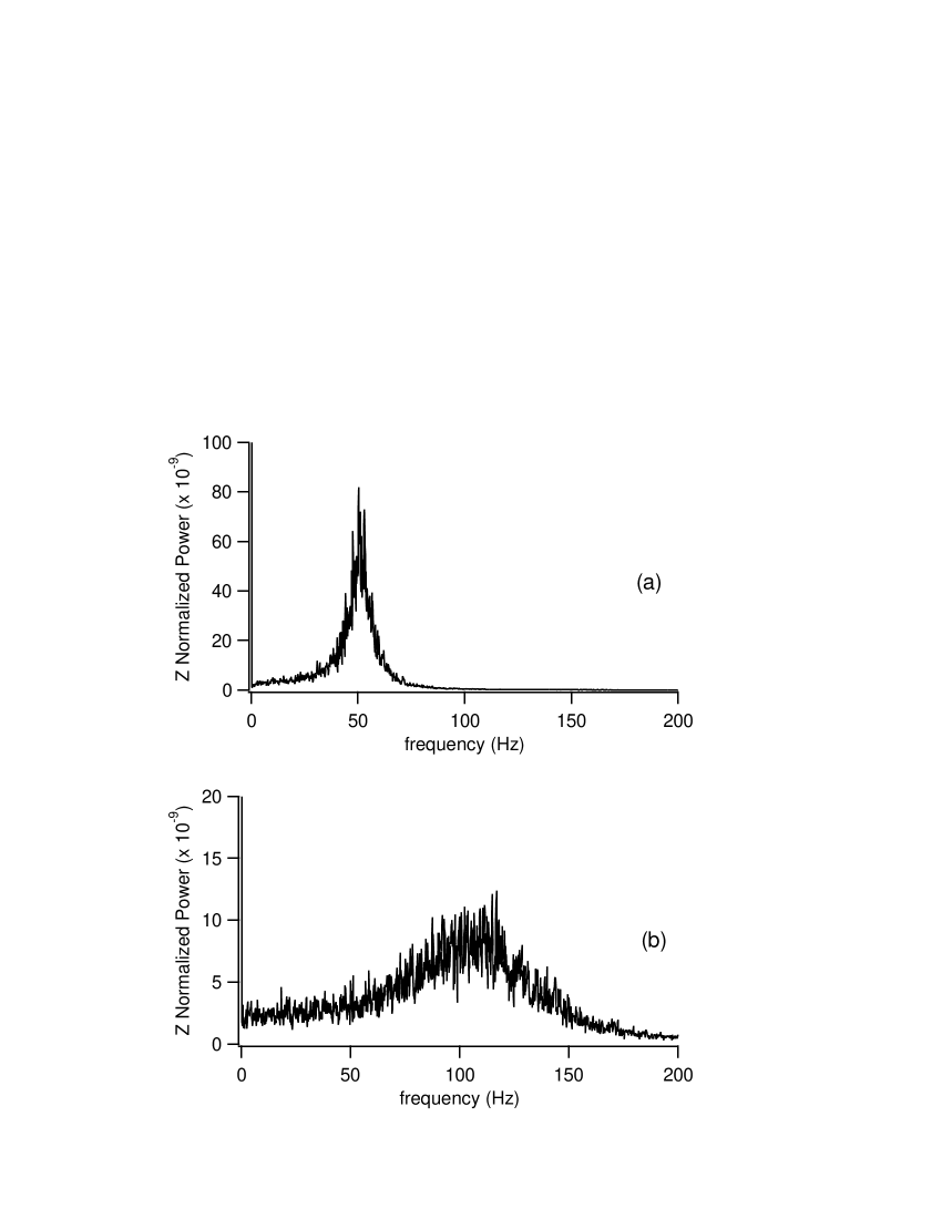
Figure 16: $Z$ spectra of the instabilities for two values of the detuning situated symmetricallty with respect to the fold maximum. In (a), $\Delta_{0}=-0.22$; in (b), $\Delta_{0}=-0.24$. Note that the vertical scale in (a) is five times larger than in (b).

The results obtained in this section can be summarized in the following way: when the parameters of the cloud are such that the unique stationary solution is stable, and therefore that no deterministic instabilities can occur, the action of noise mimics instabilities. This originates in a fold of the stationary solution, which plays the role of a noise amplifier. Moreover, the particular properties of the eigenvalues associated with the stationary solutions on the fold – small damping rate and relaxation frequency – lead to the existence of the stochastic regime: for detuning larger than the fold inflection point, a resonance is excited by the noise, leading to a dynamics with a dominating frequency; for detuning smaller than the inflection point, the damping rate increases, and the resonance vanishes. This allows us to interpret all the regimes observed experimentally.

The particular properties of the eigenvalues discussed above are in fact linked to the proximity of a Hopf bifurcation. Another known consequence of such a situation is to favor the existence of coherence resonance, and such a phenomenon exists effectively in our case nousprl . Now, an interesting question is to determine what are the exact connections between all these phenomena, and in particular if the existence of coherence resonance has a determining role in that of instabilities. The answer is obviously: no! Indeed, the essential ingredient for noise amplification is the fold; the properties of the eigenvalues only determine the time characteristics of the dynamics. In particular, we have checked that with the present model, no coherence resonance occurs when the MOT exhibits S_L instabilities.

7 Conclusion

It has been shown recently that the cloud of cold atoms obtained from a magneto-optical trap may exhibit a complex dynamics in the regime of high atomic densities. The observed behaviors can be essentially separated in two different types, depending of their nature: stochastic instabilities nousprl or deterministic instabilitiesInstDet . The aim of this paper was to describe extensively the experimentally observed stochastic dynamics, and to understand its mechanisms, through a model briefly presented in InstDet and detailed here.

A detailed analysis of the experimental results in the stochastic regime shows a variety of dynamical behaviors, which differ by the frequency components appearing in the dynamics. Indeed, some instabilities exhibit only low frequency components, while in other cases, a second time scale, corresponding to a higher frequency, appears in the motion of the center of mass of the cloud.

The simple stochastic 1D-model that we use here allows us to retrieve and interpret these experimental dynamics. The model shows that the existence of instabilities is linked to folded stationary solutions where noise response is enhanced. Moreover, the proximity of a Hopf bifurcation and the resulting conditions on the stability of the stationary solutions – small damping rate and existence of a relaxation frequency – explains the existence of several types of regimes: indeed, depending on the parameters, noise is sometimes able to excite the relaxation frequency, leading to the appearance of the second time scale in the dynamics. Globally, the agreement between this over-simplified 1D model and the 3D experiments is surprisingly good. Not only it allows us to make a qualitative interpretation of the experimentally observed dynamics, but also gives quantitative results compatible with the experimental measures, in particular concerning the amplitude of the instabilities. However, it is clear that a 3D model is necessary for an accurate quantitative description of all the experimental observations.

The model also emphasized the close relations between the stochastic and deterministic instabilities. Indeed, both types of dynamics appear to be link to the same factors: the effective dynamics depends mainly on the distance between the working point and the bistable cycles (or the Hopf bifurcation). In fact, the dynamics described in the present paper appears as the first sign of the deterministic instabilities described in InstDet , and thus may be considered as a noisy precursor to deterministic instabilitiesparamaccess ; precursor . A study of the phenomenon from this point of view should put in evidence new properties of these instabilities.

8 Acknowledgments

The author thanks M. Fauquembergue and A. di Stefano for their participation in the elaboration of the model, D. Wilkowski for its contribution to the first stages of the experiments, and Ph. Verkerk for useful discussions and his comments about this paper. The Laboratoire de Physique des Lasers, Atomes et Molécules is “Unité Mixte de Recherche de l’Université de Lille 1 et du CNRS” (UMR 8523). The Centre d’Etudes et de Recherches Lasers et Applications (CERLA) is supported by the Ministère chargé de la Recherche, the Région Nord-Pas de Calais and the Fonds Européen de Développement Economique des Régions.

References

- (1) B. G. Klappauf, W. H. Oskay, D. A. Steck, M. G. Raizen, Physica D 31, (1999) 78
- (2) Y. Sortais, S. Bize, C. Nicolas, A. Clairon, C. Salomon, C. Williams, Phys. Rev. Lett. 85, (2000) 3117
- (3) S. Chu, Rev. Mod. Phys. 70, (1998) 685; C. Cohen-Tannoudji, Rev. Mod. Phys. 70, (1998) 707; W. Phillips, Rev. Mod. Phys. 70, (1998) 721
- (4) T. Walker, D. Sesko and C. Wieman, Phys. Rev. Lett. 64, (1990) 408; D. W. Sesko, T. G. Walker and C. E. Wieman, J. Opt. Soc. Am. B 8, 946 (1991) 946
- (5) I. Guedes, M. T. de Araujo, D. M. B. P. Milori, G. I. Surdutovich, V. S. Bagnato and S. C. Zilio, J. Opt. Soc. Am. 11 (1994) 1935; V. S. Bagnato, L. G. Marcassa, M. Oria, R. Vitlina, and S. Zilio, Phys. Rev. A 48, (1993) 3771
- (6) S. Bielawski, M. Bouazaoui, D. Derozier, P. Glorieux, Phys. Rev. A 47, (1993 3276); N. Joly and S. Bielawski, Opt. Lett. 26, (2001) 692
- (7) S. Bielawski, D. Derozier, P. Glorieux, Phys. Rev. A 47, (1993 R2492); A. N. Pisarchik and B. K. Goswami, Phys. Rev. Lett. 84, (2000) 1423
- (8) see e.g. Edward Ott, Chaos in dynamical systems Cambridge University Press, Cambridge (1993)
- (9) D. Wilkowski, J. Ringot, D. Hennequin and J. C. Garreau, Phys. Rev. Lett. 85, (2000) 1839
- (10) A. di Stefano, M. Fauquembergue, Ph. Verkerk and D. Hennequin, Phys. Rev. A 67, (2003)
- (11) J. Dalibard, Opt. Commun. 68, (1988) 203
- (12) D. Wilkowski, J. C. Garreau and D. Hennequin, Eur. Phys. J. D 2, (1998) 157
- (13) C. G. Townsend, N. H. Edwards, C. J. Cooper, K. P. Zetie, C. J. Foot, A. Steane, P. Szriftgiser, H. Perrin and J. Dalibard, Phys. Rev. A 52, (1995) 1423
- (14) L. Marcassa, V. Bagnato, Y. Wang, C. Tsao, J. Weiner, O. Dulieu, Y. B. Band and P. S. Julienne, Phys. Rev. A 47, (1993) R4563
- (15) L. Gammaitoni, P. Hänggi, P. Jung and F. Marchesoni, Rev. Mod. Phys. 70, (1998) 223
- (16) Lin I and Jeng-Mei Liu, Phys. Rev. Lett. 74, (1995) 3161
- (17) A. S. Pikovsky and J. Kurths, Phys. Rev. Lett. 78, (1997) 775
- (18) A. Neiman, P. I. Saparin and L. Stone, Phys. Rev. E 56, (1997) 270
- (19) P. Khandokin, Ya. Khanin, J.-C. Celet, D. Dangoisse and P. Glorieux, Opt. Commun. 123, (1996) 372
- (20) T. W. Carr, L. Billings, I. B. Schwartz, I. Triandaf, Physica D 147, (2000) 59