Abstract

Environmental signals sensed by nervous systems are often represented in spike trains carried from sensory neurons to higher neural functions where decisions and functional actions occur. Information about the environmental stimulus is contained (encoded) in the train of spikes. We show how to “read” the encoding using state space methods of nonlinear dynamics. We create a mapping from spike signals which are output from the neural processing system back to an estimate of the analog input signal. This mapping is realized locally in a reconstructed state space embodying both the dynamics of the source of the sensory signal and the dynamics of the neural circuit doing the processing. We explore this idea using a Hodgkin-Huxley conductance based neuron model and input from a low dimensional dynamical system, the Lorenz system. We show that one may accurately learn the dynamical input/output connection and estimate with high precision the details of the input signals from spike timing output alone. This form of “reading the neural code” has a focus on the neural circuitry as a dynamical system and emphasizes how one interprets the dynamical degrees of freedom in the neural circuit as they transform analog environmental information into spike trains.

1 Introduction

A primary task of nervous systems is the collection at its periphery of information from the environment and the distribution of that stimulus input to central nervous system functions. This is often accomplished through the production and transmission of action potentials or spike trains [16].

The book [16] and subsequent papers by its authors and their collaborators [2] carefully lay out a program for interpreting the analog stimulus of a nervous system using ideas from probability theory and information theory, as well as a representation of the input/output or stimulus/response relation in terms of Volterra kernel functions. In [16] the authors note that when presenting a stimulus to a neuron, it is common “that the response spike train is not identical on each trial.” Also they observe that “Since there is no unique response, the most we can say is that there is some probability of observing each of the different possible responses.” This viewpoint then underlies the wide use of probabilistic ideas in describing how one can “read the neural code” through interpreting the response spike trains to infer the stimulus.

In this paper we take a different point of view and recognize that the neuron into which one sends a stimulus is itself a dynamical system with a time dependent state which will typically be different upon receipt of different realizations of identical stimulus inputs. Viewing the transformation of the stimulus waveform into the observed response sequence, as a result of deterministic dynamical action of the neuron one can attribute the variation in the response to identical stimuli to differing neuron states when the stimulus arrives. This allows us to view the entire transduction process of analog input (stimulus) to spike train output (response) as a deterministic process which can be addressed by methods developed in nonlinear dynamics for dealing with input/output systems [14].

Previous research on information encoding in spike trains has concentrated on nonlinear filters that convert analog input signals into spike trains. It has been shown that these models can be used to reconstruct the dynamical phase space of chaotic inputs to the filters using the spike timing information [17, 4, 9, 10]. Using simple dynamical neuron models, Castro and Sauer [5] have shown that aspects of a dynamical system can be reconstructed using interspike intervals (ISIs) properties. Experimental work has demonstrated the ability to discriminate between chaotic and stochastic inputs to a neuron [15], as well as showing that decoding sensory information from a spike train through linear filtering Volterra series techniques can allow for large amounts of information to be carried by the precise timing of the spikes [16].

We discuss here the formulation of input/output systems from a dynamical system point of view, primarily summarizing earlier work [14, 1], but with a focus on recognizing that we may treat the response signals as trains of identical spikes. Since the modulation of the spike train must be carrying the information in the analog input presented to the neuron, if the spike pulse shapes are identical, all information must be encoded in the ISIs. We shall show that this is, indeed, the case.

What is the role of information theory in a deterministic chain of actions from stimulus to spiking response? The ideas of information theory, though often couched in terms of random variables, applies directly to distributed variation in dynamical variables such as the output from nonlinear systems. The use of concepts such as entropy and mutual information, at the basis of information theoretic descriptions of systems, applies easily and directly to deterministic systems. The understanding of this connection dates from the 1970’s and 1980’s where the work of Fraser [6] makes this explicit, and the connection due to Pesin [11] between positive Lyapunov exponents of a deterministic system and the Kolmogorov-Sinai entropy quantifies the correspondence.

In the body of this paper, we first summarize the methods used to determine a connection between analog input signals and spiking output, then we apply these methods to a Hodgkin-Huxley conductance based model of the R15 neuron of Aplysia [3, 12]. Future papers will investigate the use of these methods on biological signals from the H1 visual neuron of a fly and a stretch receptor in the tail of a crayfish [20]

2 Input Estimation from State Space Reconstruction

The general problem we address is the response to stimuli of a neural circuit with N dynamical variables

$$\mathbf{x}(t)=[x_{1}(t),x_{2}(t),\ldots,x_{N}(t)].$$

When there is no time varying input, $\mathbf{x}(t)$ satisfies the ordinary differential equations

$$\frac{dx_{a}(t)}{dt}=F_{a}(\mathbf{x}(t)),\,\,\,;a=1,2,...,N$$ (1)

The $F_{a}(\mathbf{x})$ are a set of nonlinear functions which determine the dynamical time course of the neural circuit. The $F_{a}(\mathbf{x})$ could well represent a conductance based neural model of the Hodgkin-Huxley variety as in our example below.

When there is a time dependent external stimulus $s(t)$, these equations become

$$\frac{dx_{a}(t)}{dt}=F_{a}(\mathbf{x}(t),s(t)),$$ (2)

and the time course of $\mathbf{x}(t)$ in this driven or non-autonomous setting can become rather more complicated than the case where $s(t)=\mbox{constant}$.

If we knew the dynamical origin of the signal $s(t)$, then in the combined space of the stimuli and the neural state space $\mathbf{x}(t)$, we would again have an autonomous system, and many familiar [1] methods for analyzing signals from nonlinear systems would apply. As we proceed to our “input signal from spike outputs” connection we imagine that the stimulus system is determined by some other set of state variables $\mbox{$\bf{z}$}(t)$ and that

$$\frac{d\mbox{$\bf{z}$}(t)}{dt} = \mbox{$\bf{G}$}(\mbox{$\bf{z}$}(t))$$

$$s(t) = h(\mbox{$\bf{z}$}(t)),$$ (3)

where $\mbox{$\bf{G}$}(\mbox{$\bf{z}$})$ are the nonlinear functions determining the time course of the state $\mbox{$\bf{z}$}(t)$ and $h(\mbox{$\bf{z}$}(t))$ is the nonlinear function determining the input to the neuron $s(t)$.

With observations of just one component of the state vector $\mathbf{x}(t)$, the full dynamical structure of a system described by Equation 2 can be reconstructed in a proxy state space [8, 19]. Once the dynamics of the system is reconstructed, the mapping from state variable to input can be made in the reconstructed space. Assume the measured state variable, $r(t)=g(\mbox{{\bf x}}(t))$, is sampled at times $t_{j}$, where $j$ is an integer index. According to the embedding theorem [8, 19], the dynamics of the system can be reconstructed in an embedding space using time delayed vectors of the form

$$\mbox{$\bf{y}$}(j) = [r(t_{j}),r(t_{j}+T\tau_{s}),\ldots,r(t_{j}+(\mbox{$d_{E}$}-1)T\tau_{s})]$$ (4)

$$= [r(j),r(j+T),\dots,r(j+(\mbox{$d_{E}$}-1)T)]$$

where $d_{E}$ is the dimension of the embedding, $t_{j}=t_{0}+j\tau_{s}$, $\tau_{s}$ is the sampling time, $t_{0}$ is an initial time, and $T$ is an integer time delay. If the dimension $d_{E}$ is large enough these vectors can reconstruct the dynamical structure of the full system given in Equation 2. Each vector $\mbox{$\bf{y}$}(j)$ in the reconstructed phase space depends on the state of the input signal. Therefore a mapping should exist that associates locations in the reconstructed phase space $\mbox{$\bf{y}$}(j)$ to values of the input signal $s(t_{j})\equiv s(j):s(j)=H(\mbox{$\bf{y}$}(j))$. The map $H(\mbox{$\bf{y}$})$ is the output-to-input relation we seek.

Without simultaneous measurements of the observable $r(t)$ and the input signal $s(t)$, this mapping could not be found without knowing the differential equations that make up Equation 2. But in a situation where a controlled stimulus is presented to a neuron while measuring the output, both $r(t)$ and $s(t)$ are available simultaneously. Such a data set with simultaneous measurements of spike time and input is split into two parts: the first part, called the training set, will be used to find the mapping $H(\mbox{$\bf{y}$}(j))$ between $\mbox{$\bf{y}$}(j)$ and $s(j)$. The second part, called the test set, will be used to test the accuracy of that mapping. State variable data from the training set $r(j)$ is used to construct time delayed vectors as given by

$$\mbox{$\bf{y}$}(j)=[r(j),r(j+T),\ldots,r(j+(\mbox{$d_{E}$}-1)T)].$$ (5)

Each of these vectors is paired with the value of the stimulus at the midpoint time of the delay vector

$$s(j)=s\left(t_{j+T(\mbox{$d_{E}$}-1)/2}\right)$$ (6)

We use state space values that occur before and after the input to improve the quality of the representation. The state variables and input values in the remainder of the data are organized in a similar way and used to test the mapping.

The phase space dynamics near a test data vector are reconstructed using vectors in the training set that are close to the test vector, where we use Euclidian distance between vectors. These vectors lie close in the reconstructed phase space, so they will define the dynamics of the system in that region and will define a local map from that region to a input signal value. In other words, we seek a form for $H(\mbox{$\bf{y}$}(j))$ which is local in reconstructed phase space to $\mbox{$\bf{y}$}(j)$. The global map over all of phase space is a collection of local maps.

The local map is made using the $N_{B}$ nearest neighbors $\mbox{$\bf{y}$}^{m}(j)\;,\;m=0\ldots N_{B}$ of $\mbox{$\bf{y}$}^{0}(j)=\mbox{$\bf{y}$}(j)$. These nearest neighbor vectors and their corresponding input values $s^{m}(j)$ are used to find a local polynomial mapping between inputs $s^{m}(j)$ and vector versions of the outputs $r^{m}(j)$, namely $\mbox{$\bf{y}$}^{m}(j)$ of the form

$$s^{m}(j)=H(\mbox{$\bf{y}$}^{m}(j))=M_{0}(j)+\mbox{\bf M}_{1}(j)\cdot\mbox{$\bf{y}$}^{m}(j)+\mbox{\bf M}_{2}(j)\cdot\mbox{$\bf{y}$}^{m}(j)\cdot\mbox{$\bf{y}$}^{m}(j)+\cdots,$$ (7)

which assume that the function $H(\mbox{$\bf{y}$})$ is locally smooth in phase space.

The scalar $M_{0}(j)$, the $d_{E}$-dimensional vector $\mbox{\bf M}_{1}(j)$, and the tensor $\mbox{\bf M}_{2}(j)$ in $d_{E}$-dimensions, etc are determined by minimizing the mean squared error

$$\sum^{N_{B}}_{m=0}|s^{m}(j)-M_{0}(j)+\mbox{\bf M}_{1}(j)\cdot\mbox{$\bf{y}$}^{m}(j)+\mbox{\bf M}_{2}(j)\cdot\mbox{$\bf{y}$}^{m}(j)\cdot\mbox{$\bf{y}$}^{m}(j)+\cdots|^{2}.$$ (8)

We determine $M_{0}(j),\mbox{\bf M}_{1}(j),\mbox{\bf M}_{2}(j),\ldots$ for all $j=1,2,\ldots$, and this provides a local representation of $H(\mbox{$\bf{y}$})$ in all parts of phase space sampled by the training set $\mbox{$\bf{y}$}(j),\;j=1,2,\ldots,N_{train}$.

Once the least squares fit values of $M_{0}(j),\mbox{\bf M}_{1}(j),\mbox{\bf M}_{2}(j),\ldots$ are determined for our training set, we can use the resulting local map to determine estimates of the input associated with an observed output. This proceeds as follows: select a new output $r^{new}(l)$ and form the new output vector $\mbox{$\bf{y}$}^{new}(l)$ as above. Find the nearest neighbor in the training set to $\mbox{$\bf{y}$}^{new}(l)$. Suppose it is the vector $\mbox{$\bf{y}$}(q)$. Now evaluate an estimated input $s^{est}(l)$ as

$$s^{est}(l)=M_{0}(q)+\mbox{\bf M}_{1}(q)\cdot\mbox{$\bf{y}$}^{new}(l)+\mbox{\bf M}_{2}(q)\cdot\mbox{$\bf{y}$}^{new}(l)\cdot\mbox{$\bf{y}$}^{new}(l)+\cdots.$$ (9)

This procedure is applied for all new outputs to produce the corresponding estimated inputs.

3 R15 Neuron Model

To investigate our ability to reconstruct stimuli of analog form presented to a realistic neuron from the spike train output of that neuron, we examined a detailed model of the R15 neuron in Aplysia [3, 12], and presented this model neuron with nonperiodic input from a low dimensional dynamical system. This model has seven dynamical degrees of freedom. The differential equations for this model are

$$C\frac{dV_{m}(t)}{dt} = (g_{I}y_{2}(t)^{3}y_{3}(t)+g_{T})(V_{I}-V(t))+g_{L}(V_{L}-V(t))$$ (10)

$$+ (g_{K}y_{4}(t)^{4}+g_{A}y_{5}(t)y_{6}(t)+g_{P}y_{7}(t))(V_{K}-V(t))$$

$$+ I_{0}+I_{ext}+I_{input}(t),$$

where the $y_{n}(t);\;n=2,3,\ldots,7$ satisfy kinetic equations of the form

$$\frac{dy_{n}(t)}{dt}=\frac{Y_{n}(V_{m}(t))-y_{n}(t)}{\tau_{n}(V_{m}(t))},$$ (11)

which is the usual form of Hodgkin-Huxley models. The $g_{X},X=I,T,K,A,P,L$ are maximal conductances, the $V_{X},X=I,L,K$ are reversal potentials. $V_{m}(t)$ is the membrane potential, $C$ is the membrane capacitance, $I_{0}$ is a fixed DC current, and $I_{ext}$ is a DC current we vary to change the state of oscillation of the model. The functions $Y_{n}(V)$ and $\tau_{n}(V)$ and values for the various constants are given in [3, 12]. These are phenomenological forms of membrane voltage dependent gating variables, activation and inactivation of membrane ionic channels, and time constants for these gates. $I_{input}(t)$ is a time varying current input to the neural dynamics. Our goal will be to reconstruct $I_{input}(t)$ from observations of the spike timing in $V_{m}(t)$.

In Figure 1 we plot the bifurcation diagram of our R15 model. On the vertical axis we show the values of ISIs taken in the time series for $V_{m}(t)$ from the model; on the horizontal axis we plot $I_{ext}$. From this bifurcation plot we see that the output of the R15 model has regular windows for $I_{ext}<.07$ then chaotic regions interspersed with periodic orbits until $I_{ext}\approx 0.19$ after which nearly periodic behavior is seen. The last region represents significant depolarization of the neuron in which tonic periodic firing associated with a stable limit cycle in phase space is typical of neural activity. Periodic firing leads to a fixed value for ISIs, which is what we see. Careful inspection of the time series reveals very small fluctuations in the phase space orbit, but the resolution in Figure 1 does not expose this.

Other than the characteristic spikes, there are no significant features in the membrane voltage dynamics. In addition all the spikes are essentially the same, so we expect that all the information about the membrane voltage state is captured in the times between spikes, namely the interspike intervals: ISIs. The distribution of ISIs characterizes the output signal for information theoretic purposes.

We have chosen three values of $I_{ext}$ at which to examine the response of this neuron model when presented with an input signal. At $I_{ext}=0.1613$ we expect chaotic waveforms expressed as nonperiodic ISIs with a broad distribution. At $I_{ext}=0.2031$ we expect nearly periodic spike trains. And at $I_{ext}=-0.15$ the neuron does not spike, the mebrane voltage remains at an equilibrium value.

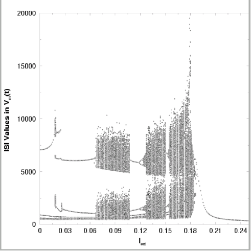
Figure 1: Bifurcation diagram for the R15 model with constant input current. This plot shows the values of ISIs which occur in the $V_{m}(t)$ time series for different values of $I_{ext}$.

For each $V_{m}(t)$ time series we evaluate the normalized distribution of ISIs which we call $P_{ISI}(\Delta)$ and from this we compute the entropy associated with the oscillations of the neuron. Entropy is defined as

$$H(\Delta)=\sum_{\mbox{observed}\,\Delta}-P_{ISI}(\Delta)\log\biggl{(}P_{ISI}(\Delta)\biggr{)};$$ (12)

$H(\Delta)\geq 0$. The entropy is a quantitative measure [18] of the information content of the output signal from the neural activity.

In Figure 2 we display a section of the $V_{m}(t)$ time series for $I_{ext}=0.1613$. The irregularity in the spiking times is clear from this figure and the distribution $P_{ISI}(\Delta)$ shown in Figure 3. The $P_{ISI}(\Delta)$ was evaluated from collecting 60,000 spikes from the $V_{m}(t)$ time series and creating a histogram with 15,000 bins. This distribution has an entropy $H(\Delta)=12$. In contrast to this we have a section of the $V_{m}(t)$ time series for $I_{ext}=0.2031$ in Figure 4. Far more regular firing is observed with a firing frequency much higher than for $I_{ext}=0.1613$. This increase in firing frequency as a neuron is depolarized is familiar. With $I_{ext}=0.2031$ the distribution $P_{ISI}(\Delta)$ is mainly concentrated in one bin with some small flucuations near that bin. Such a regular distribution leads to a very low entropy $H(\Delta)=0.034$. If not for the slight variations in ISI, the entropy would be zero. If $P_{ISI}(\Delta_{0})=1$ for some ISI value $\Delta_{0}$, then $H(\Delta)=0$.

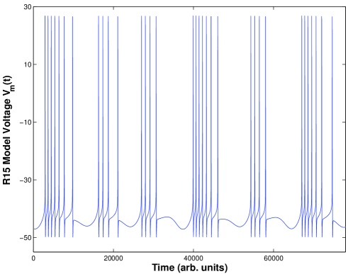
Figure 2: Membrane voltage of the R15 model with a constant input current $I_{ext}$ = 0.1613.

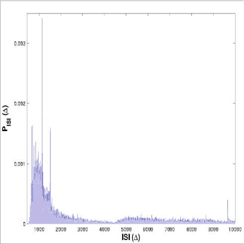
Figure 3: Normalized distribution $P_{ISI}(\Delta)$ from the membrane voltage time series with $I_{ext}$ = 0.1613. The entropy for this distribution $H(\Delta)=12$.

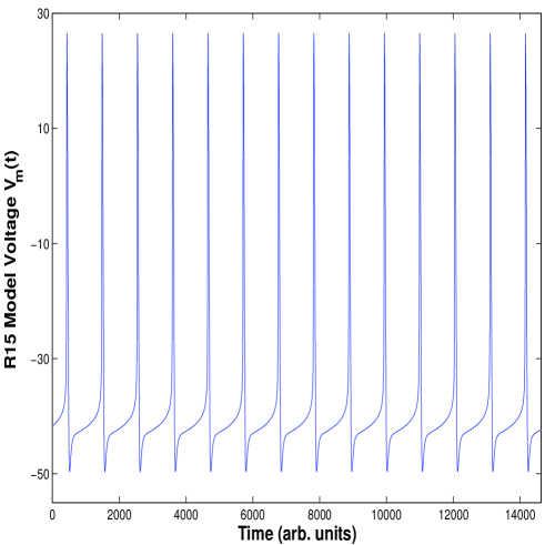
Figure 4: Membrane voltage of the R15 model with a constant input current $I_{ext}$ = 0.2031.

3.1 Input Signals to Model Neuron

In the last section the dynamics of the neuron model were examined using constant input signals. In studying how neurons encode information in their spike train, we must clarify what it means for a signal to carry information. In the context of information theory [18], information lies in the unpredictability of a signal. If we do not know what a signal is going to do next, then by observing it we gain new information. Stochastic signals are commonly used as information carrying signals since their unpredictability is easily characterized and readily incorporated into the theoretical structure of information theory. But they are problematic when approaching a problem from a dynamical systems point of view, since they are systems with a high dimension. This means that the reconstruction of a stochastic signal using time delay embedding vectors of the form of Equation 4 would require an extremely large embedding dimension [1]. If we are injecting stochastic signals into the R15 model, the dimension of the whole system would increase and cause practical problems in performing the input reconstruction. Indeed, the degrees of freedom in the stochastic input signal could well make the input/output relationship we seek to expose impossible to see.

An attractive input for testing the reconstruction method will have some unpredictability but have few degrees of freedom. If there are many degrees of freedom, the dimensionality of the vector of outputs $\mbox{$\bf{y}$}(j)$ above may be prohibitively large. This leads directly to the consideration of low dimensional chaotic systems. Chaos originates from local instabilities which cause two points initially close together in phase space to diverge rapidly as the system evolves in time, thus producing completely different trajectories. This exponential divergence is quantified by the positive Lyapunov exponents and is the source of the unpredictability in chaotic systems [1]. The state of any observed system is known only to some degree of accuracy, limited by measurement and systematic errors. If the state of a chaotic system were known exactly then the future state of that system should be exactly predictable. But if the state of a chaotic system is only known to some finite accuracy, then predictions into the future based on the estimated state will diverge from the actual evolution of the system. Imperfect observations of a chaotic signal will limit the predictability of the signal. Since chaos can occur in low dimensional systems these signals do not raise the same concerns as stochastic signals.

We use a familiar example of a chaotic system, the Lorenz attractor [7], as the input signal to drive the R15 model. This is a well studied system that exhibits chaotic dynamics and will be used here as input to the R15 neuron model. The Lorenz attractor is defined by the differential equations

$$\kappa\frac{dx(t)}{dt} = \sigma(y(t)-x(t))$$

$$\kappa\frac{dy(t)}{dt} = -x(t)z(t)+rx(t)-y(t)$$ (13)

$$\kappa\frac{dz(t)}{dt} = x(t)y(t)-bz(t)$$

For the simulations presented in this paper the parameters were chosen as $\sigma=16$, $r=45.92$ and $b=4$. The parameter $\kappa$ is used to change the time scale. An example times series of the $x(t)$ component of the Lorenz attractor is shown in Figure 5.

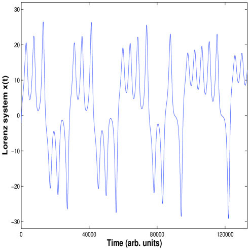
Figure 5: Small segment of the $x(t)$ component of the Lorenz attractor described in equations 3.1 with $\kappa=10^{4}$.

3.2 Numerical Results

An input signal $s(t)=I_{input}(t)$ is now formed from the $x(t)$ component of the Lorenz system. Our goal is to use observations of the stimulus $I_{input}(t)$ and of the ISIs of the output signal $V_{m}(t)$ to learn the dynamics of the R15 neuron model in the form of a local map in phase space reconstructed from the observed ISIs. From this map we will estimate the input $I_{input}(t)$ from new observations of the output ISIs.

Our analog signal input is the $x(t)$ output of the Lorenz system, scaled and offset to a proper range, and then input to the neuron as an external current

$$I_{input}(t)=\mbox{Amp}(x(t)+x_{0}),$$ (14)

where Amp is the scaling constant and $x_{0}$ is the offset. The R15 equations are integrated [13] with this input signal and the spike times $t_{j}$ from the membrane voltage are recorded simultaneously with the value of the input current at that time $I_{input}(t_{j})$. Reconstruction of the neuron plus input phase space is done by creating time delay vectors from the ISIs

$$\mbox{$\bf{y}$}(j)=[isi_{j},isi_{j+1},\ldots,isi_{j+(\mbox{$d_{E}$}-1)\tau}]$$ (15)

where

$$isi_{j}=t_{j}-t_{j-1}$$ (16)

For each of these vectors there is a corresponding value of the input current which we chose to be at the midpoint time of the vector

$$s(j)=I_{input}\left(t_{j+(\mbox{$d_{E}$}-1)\tau/2}\right)$$ (17)

In our work a total of 40000 spikes were collected. The first 30000 were used to create the training set vectors and the next 10000 were used to examine our input estimation methods. For each new output vector constructed from new observed ISIs, $N_{B}$ nearest neighbors from the training set were used to generate a local polynomial map $\mbox{$\bf{y}$}(j)\to I^{estimated}_{input}(j)$. $N_{B}$ was chosen to be twice the number of free parameters in the undetermined local coefficients $M_{0},\mbox{\bf M}_{1},\mbox{\bf M}_{2},\ldots$.

We used the same three values of $I_{ext}$ -0.15, 0.1613, and 0.2031 employed above in our simulations. We took $\mbox{Amp}=0.001$, $\kappa=10^{4}$, and $x_{0}=43.5$ for all simulations unless stated otherwise. This very small amplitude of the input current is much more of a challenge for the input reconstruction than large amplitudes. When Amp is large, the neural activity is entrained by the input signal and ‘recovering’ the input merely requires looking at the output and scaling it by a constant. Further, the intrinsic spiking of the neuron which is its important biological feature goes away when Amp is large. The large value of $\kappa$ assures that the spikes sample the analog signal $I_{input}(t)$ very well.

For $I_{ext}=0.1613$ we show a selection of both the input current $I_{input}$ and the output membrane voltage $V_{m}(t)$ time series in Figure 6. The injected current substantially changes the pattern of firing seen for the autonomous neuron. Note that the size of the input current is numerically about $10^{-3}$ of $V_{m}(t)$, yet the modulation of the ISIs due to this small input is clearly visible in Figure 6.

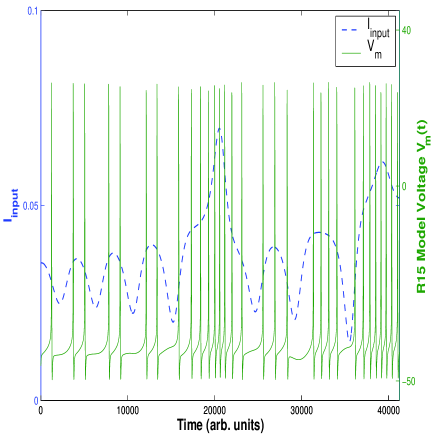
Figure 6: A segment of the R15 neuron model output $V_{m}(t)$ shown along with the scaled Lorenz system input current $I_{input}$. Here $I_{ext}=0.1613$, $\mbox{Amp}=0.001$, and $\kappa=10^{4}$. Note the different scales for $I_{input}$ (shown on the left axis) and $V_{m}(t)$. (shown on the right axis)

Using the ISIs of this time series we evaluated $P_{ISI}(\Delta)$ as discussed above and from that the entropy $H(\Delta)$ associated with the driven neuron. The ISI distribution, $P_{ISI}(\Delta)$, shown in Figure 7, has an entropy $H(\Delta)=8.16$. The effect of the input current has been to substantially narrow the range of ISIs seen in $V_{m}(t)$. This can be seen by comparison with Figure 3.

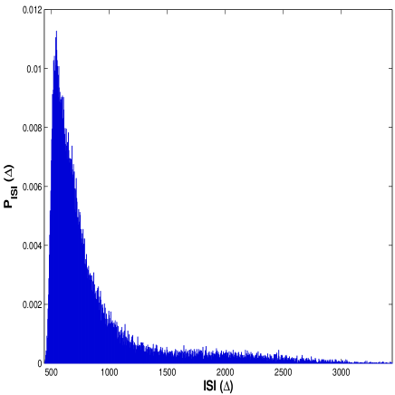
Figure 7: $P_{ISI}(\Delta)$ for R15 model neuron output when a scaled $x(t)$ signal from the Lorenz system is presented with $I_{ext}=0.1613$. The entropy of this distribution $H(\Delta)=8.16$.

Figure 8 shows an example of input signal reconstruction which estimates $I_{input}$ using ISI vectors of the described in Equation 15. We used a time delay $T=1$, an embedding dimension $\mbox{$d_{E}$}=7$, and a local linear map for $H(\mbox{$\bf{y}$}(j))$. The RMS error over the 10,000 reconstructed values of the input was $\sigma=4.6\cdot 10^{-4}$. The input signal is only reconstructed at times at which the neuron spikes. So each point is the reconstruction curve in Figure 8 corresponds to a spike in $V_{m}(t)$. Some features of the input are missed because no spikes occur during that time, but otherwise the reconstruction is very accurate. At places where the spike rate is high, interpolation seems to fill the gaps between spikes.

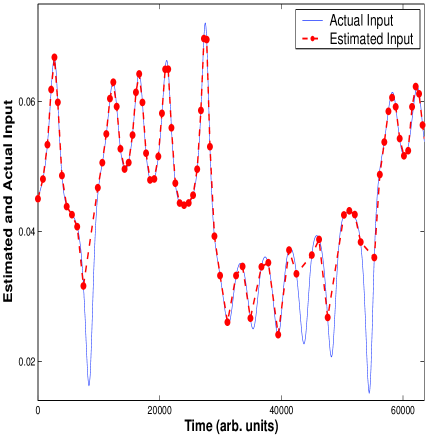
Figure 8: ISI Reconstruction of the input Lorenz signal to an R15 neuron. The solid line is the actual input to the neuron. The dots joined by dashed lines are the ISI reconstructions. The embedding dimension of the reconstruction $d_{E}$ is 4, the time delay $T$ is 1, $I_{ext}=0.1613$, $\kappa$ is $10^{4}$, and a linear map was used. The RMS error of the estimates over 10,000 estimations is $\sigma=4.6\cdot 10^{-4}$ and the maximum error is about $0.01$.

Different values of embedding dimension, time delay, and map order will lead to different reconstruction errors. For example, low embedding dimension may not unfold the dynamics and linear maps may not be able to fit some neighborhoods to the input. For the results shown here, there is little difference in the RMS reconstruction error if the embedding dimension is increased or quadratic maps are used instead of linear maps. This may not be true if lower embedding dimension is used.

The previous example probed the response of a chaotic neural oscillation to a chaotic signal. With $I_{ext}=0.2031$ the neuron is in a periodic spiking regime and the input modulates the instantaneous firing rate of the neuron. A sample of the input current and membrane voltage is shown in Figure 9. The distribution of ISIs, $P_{ISI}(\Delta)$, shown in Figure 10 and has an entropy $H(\Delta)=9.5$. The effect of the input current is to substantially broaden the range of ISIs and increase its entropy as compared to the nearly periodic firing of the autonomous neuron with $I_{ext}=0.2031$. The high spiking rate and close relationship between input current amplitude and ISI lead to very accurate reconstructions using low dimensional embeddings. A sample of the reconstruction using $\mbox{$d_{E}$}=2$ and $T=1$ is shown in Figure 11. The RMS reconstruction error of $\sigma=6.1\cdot 10^{-4}$ with a maximum error of $0.007$.

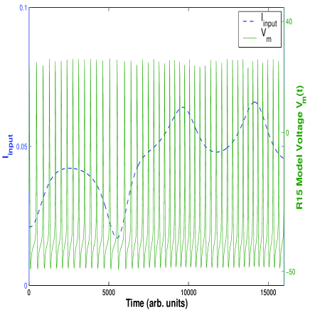
Figure 9: A segment of the R15 neuron model output $V_{m}(t)$ shown along with the scaled Lorenz system input current $I_{input}$. Here $I_{ext}=0.2031$,$\mbox{Amp}=0.001$, and $\kappa=10^{4}$. Note the different scales for $I_{input}$ and $V_{m}(t)$.

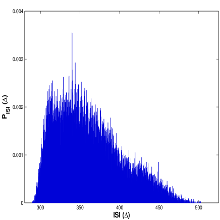
Figure 10: $P_{ISI}(\Delta)$ for R15 model neuron output when a scaled $x(t)$ signal from the Lorenz system is presented with $I_{ext}=0.2031$. The entropy of this distribution $H(\Delta)=9.5$.

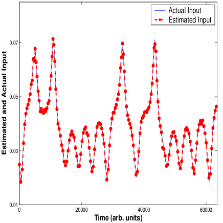
Figure 11: ISI Reconstruction of the input Lorenz signal to an R15 neuron. The solid line is the actual input to the neuron. The dots joined by dashed lines are the ISI reconstructions. The embedding dimension of the reconstruction $d_{E}$ is 2, the time delay $T$ is 1, $I_{ext}=0.2031$, $\kappa$ is $10^{4}$, and a linear map was used. The RMS error of the estimates over 10,000 estimations is $\sigma=6.1\cdot 10^{-4}$ and the maximum error is about $0.007$.

In a final example we show the reconstruction when the neuron is being driven with an input current below the threshold for spikes. With $I_{ext}=-0.15$, the autonomous R15 neuron will remain at an equilibrium level and not produce spikes. A Lorenz input injected into the neuron with $\mbox{Amp}=0.002$ and $x_{0}=43.5$ is large enough to cause the neuron to spike. Figure 12 shows a sample of the membrane voltage time series along with the corresponding input current. Since the spiking rate of the neuron is much lower than before, $\kappa$ is increased to $2\cdot 10^{5}$. This slows down the dynamics of the Lorenz input relative to the neuron dynamics. Spikes occur during increasing portions of the input current and are absent for low values of input current. Figure 13 shows the distribution of ISIs which has an entropy $H(\Delta)=5.3$. The low spiking rate shows up in the distribution in the form large numbers of long ISI. For the reconstruction of the input larger embedding dimensions were needed. An sample of the reconstruction is shown in Figure 14 using $\mbox{$d_{E}$}=7$ and $T=1$. For this fit the RMS reconstruction error $\sigma=0.0094$ with a maximum error of $0.03$. These errors are noticeably higher than the previous two examples.

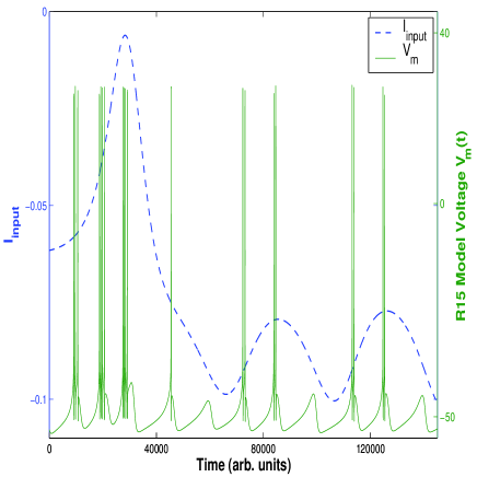
Figure 12: A segment of the R15 neuron model output $V_{m}(t)$ shown along with the scaled Lorenz system input current $I_{input}$. Here $I_{ext}=-0.15$,$\mbox{Amp}=0.002$, and $\kappa=2\cdot 10^{5}$. Note the different scales for $I_{input}$ and $V_{m}(t)$.

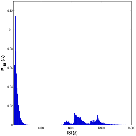
Figure 13: $P_{ISI}(\Delta)$ for R15 model neuron output when a scaled $x(t)$ signal from the Lorenz system is presented with $I_{ext}=-0.15$. The entropy of this distribution $H(\Delta)=5.3$.

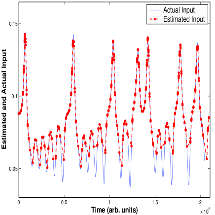
Figure 14: ISI Reconstruction of the input Lorenz signal to an R15 neuron. The solid line is the actual input to the neuron. The dots joined by dashed lines are the ISI reconstructions. The embedding dimension of the reconstruction $d_{E}$ is 7, the time delay $T$ is 1, $I_{ext}=-0.15$, $\kappa$ is $2\cdot 10^{5}$, and a linear map was used. The RMS error of the estimates over 10,000 estimations is $\sigma=0.0094$ and the maximum error is about $0.03$.

The accuracy of the reconstruction method depends on a high spiking rate in the neuron relative to the time scale of the input signal, since only one reconstructed input value is generated for each spike. If the spiking rate of the neuron is low relative to the time scales of the input signal, then the neuron will undersample the input signal and miss many of its features. This limitation can be demonstrated by decreasing the time scale parameter $\kappa$, thereby speeding up the dynamics of the input. During the longer ISIs the input current can change by large amounts. Though the reconstruction undersamples the input, but interpolation can fill in some of the gaps. As $\kappa$ is increased further the reconstruction will further degrade.

4 Discussion

In previous research on the encoding of chaotic attractors in spikes trains, the spike trains were produced by nonlinear transformations of chaotic input signals. Threshold crossing neuron models have been used, which generate the spike times at upward crossings of a threshold. This is equivalent to a Poincare section of the input signal. Also integrate and fire neurons have been studied, which integrate the input signal and fire a spike when it crosses a threshold, after which the integral is reset to zero. Both of these models have no intrinsic complex dynamics; they can not produce entropy autonomously. All of the complex behavior is in the input signal. Even though the attractor of a chaotic input can be reconstructed from the ISIs, these models do not account for the complex behavior of real neurons. The input reconstruction method we have presented here allows for complex intrinsic dynamics of the neuron. We have shown that the local polynomial representations of input/output relations realized in reconstructed phase space can extract the chaotic input from the complex interaction between the input signal and neuron dynamics.

Other experimental works have used linear kernels to map the spike train into the input. They have shown that the precise timing of individual spikes can encode a lot of information about the input [16]. And the precise relative timing between two spikes can carry even more information than their individual timings combined [2]. These results may be pointing toward a state space representation since the time delay embedding vectors used here take into account both the precise spike timing and the recent history of ISIs. From a dynamical systems perspective this is important because the state of the system at the time of the input will affect its response. This is a factor that linear kernels do not take into account.

The advantage of using local representations of input/output relations in reconstructed state space lies primarily in the insight it may provide about the underlying dynamics of the neural transformation process mapping analog environmental signals into spike trains. The goal of the work presented here is not primarily to show we can accurately recover analog input signals from the ISIs of spike output from neurons, though that is important to demonstrate. The main goal is to provide clues on how one can now model the neural circuitry which transforms these analog signals. The main piece of information in the work presented here lies in the size of the reconstructed space $d_{E}$ which tells us something about the required dimension of the neural circuit. Here we see that a low dimension can give excellent results indicating that the complexity of the neural circuit is not fully utilized in the transformation to spikes. Another suggestion of this is in the entropy of the input and output signals. In the case where $I_{ext}=0.1613$ the entropy of the analog input is $11.8$ while the entropy of the ISI distribution of the output is $8.16$. When $I_{ext}=0.2031$ the output entropy is $9.5$. This suggests, especially in the case of the larger current, that the signal into R15 neuron model acts primarily as a modulation on the ISI distribution. This modulation may be substantial, as in the case when $I_{ext}=0.1613$ but reading the modulated signal does not require complex methods.

Our final example took $I_{ext}=-0.15$ at which value the undriven neuron has $V_{m}(t)=\mbox{constant}$, so it is below threhold for production of action potentials. In this case the introduction of the stimulus drove the neuron above this threshold and produced a spike train which could be accurately reconstructed. This example is relevant to the behavior of biological neurons which act as sensors for various quantities: visiual stimuli, chemical stimuli (olfaction), etc. In the study of biological sensory systems [20] the neural circuitry is quiet in the absence of input signals, yet as we now see the methods are equally valid and accurate.

References

- [1] H. D. I. Abarbanel. The Analysis of Observed Chaotic Data. Springer, New York, 1996.
- [2] N. Brenner, S. P. Strong, R. Koberle, W. Bialek, and R. de Ruyter van Steveninck. Synergy in a neural code. Neural Computation, 12:1531–52, 2000.
- [3] C. C. Canavier, J. W. Clark, and J. H. Byrne. Routes to chaos in a model of a bursting neuron. Biophys. J., 57:1245–51, 1990.
- [4] R. Castro and T. Sauer. Correlation dimension of attractors through interspike intervals. Phys. Rev. E, 55(1):287–90, 1997.
- [5] R. Castro and T. Sauer. Reconstructing chaotic dynamics through spike filters. Phys. Rev. E, 59(3):2911–17, 1999.
- [6] A. M. Fraser. Information Theory and Strange Attractors. PhD thesis, University of Texas, Austin, May 1989.
- [7] E. N. Lorenz. Deterministic nonperiodic flow. J. Atmos. Sci., 20:130–41, 1963.
- [8] R. Mañé. On the dimension of the compact invariant sets of certain nonlinear maps. In D. Rand and L. S. Young, editors, Dynamical Systems and Turbulence, Warwick, 1980, volume 898, page 230, Berlin, 1981. Springer.
- [9] A. N. Pavlov, O. V. Sosnovtseva, E. Mosekilde, and V. S. Anishcenko. Extracting dynamics from threshold-crossing interspike intervals: Possibilities and limitations. Phys. Rev. E, 61:5033–44, 2000.
- [10] A. N. Pavlov, O. V. Sosnovtseva, E. Mosekilde, and V. S. Anishcenko. Chaotic dynamics from interspike intervals. Phys. Rev. E, 63:036205, 2001.
- [11] Ya. B. Pesin. Lyapunov characteristic exponents and smooth ergodic theory. Usp. Mat. Nauk., 32:55, 1977. English translation in Russian Math. Survey, Volume 72, 55, (1977).
- [12] R. E. Plant and M. Kim. Mathematical description of a bursting pacemaker neuron by a modification of the hodgkin-huxley equations. Biophys. J., 16:227–44, 1976.
- [13] W. H. Press, S. A. Teukolsky, W. T. Vetterling, and B. P. Flannery. Numerical Recipes in FORTRAN. Cambridge University Press, Cambridge, 1992.
- [14] C. Rhodes and M. Morari. Determining the model order of nonlinear input/output systems. AIChE J., 44:151–63, 1998.
- [15] K. A. Richardson, T. T. Imhoff, P. Grigg, and J. J. Collins. Encoding chaos in neural spike trains. Phys. Rev. Lett., 80:2485–88, 1998.
- [16] F. Rieke, D. Warland, R. de Ruyter van Steveninck, and W. Bialek. Spikes : Exploring the Neural Code. The MIT Press, Cambridge, MA, 1997.
- [17] T. Sauer. Reconstructing of dynamical systems from interspike intervals. Phys. Rev. Lett., 72(24):3811–14, 1994.
- [18] C. E. Shannon. A mathematical theory of communication. Bell Syst. Tech. J., 27:379–423 and 623–656, 1948.
- [19] F. Takens. Detecting strange attractors in turbulence. In D. Rand and L. S. Young, editors, Dynamical Systems and Turbulence, Warwick, 1980, volume 898, page 366, Berlin, 1981. Springer.
- [20] E. C. Tumer, J. H. Wolfe, K. Wood, H. D. I. Abarbanel, M. I. Rabinovich, and A. I. Selverston. Reading neural codes : The importance of spike patterns. To be submitted to Nature Neuroscience September 2002, 2002.