Analytical study of the effect of recombination on evolution via DNA shuffling

Abstract

We investigate a multi-locus evolutionary model which is based on the DNA shuffling protocol widely applied in in vitro directed evolution. This model incorporates selection, recombination and point mutations. The simplicity of the model allows us to obtain a full analytical treatment of both its dynamical and equilibrium properties, for the case of an infinite population. We also briefly discuss finite population size corrections.

Recombination of genetic information is a widespread phenomena in both prokaryotes and eukaryotes. In prokaryotes, recombination occurs in the forms of transformation, virus aided transduction, and conjugation. In eukaryotes, recombination between homologous sequences is a fundamental component underlying sexual reproduction (e.g., LODISH et.al. $1999$). An enormous body of research has been devoted to understanding the evolutionary benefit of recombination in various circumstances. This effort has led to some general understanding of the circumstances under which recombination helps facilitate evolution, although many important questions still remain open (OTTO and LENORMAND $2002$).

Inspired by recombination in natural evolution, and propelled by advances in biotechnology, recombination has been employed in in vitro molecular evolution experiments to develop novel proteins and DNA sequences (e.g., KURTZMAN et.al. $2001$; FARINAS et.al. $2001$). This family of evolutionary protocols, called DNA shuffling (or molecular breeding) (STEMMER $1994$a; $1994$b), has been shown experimentally to produce, in terms of the rate of evolutionary progression and final product quality, far superior results as compared to conventional directed evolution methods using only mutagenesis (e.g., KURTZMAN et.al. $2001$; FARINAS et.al. $2001$). In addition to its widespread practical applications, DNA shuffling (as an approach of in vitro evolution) has been used to mimic natural evolutionary processes and predict possible evolutionary pathways (ORENCIA et.al. $2001$; BARLOW and HALL $2002$).

In spite of its enormous significance, theoretical understanding of DNA shuffling has been lacking. In this paper, we investigate DNA shuffling from the perspective of evolutionary modelling. Specifically, we aim to find out, quantitatively and analytically, the benefit that the extra step of recombination provides in the evolutionary process, as well as such aspects as the role of mutation and finite population effects.

Compared to other evolutionary models, DNA shuffling has two unique aspects that render it attractive to study. First, the methods of biotechnology enable a unique recombination scheme that goes well beyond the classical one, i.e., two parents with at most a few crossovers. This multi-parent multi-crossover nature of DNA shuffling, as we shall see, makes it more effective, and also, incidentally, dramatically simplifies the analytical treatment. Second, in the setting of DNA shuffling the relationship between genotype, phenotype and fitness is relatively clear and well-defined. In addition, such parameters as selection strength, mutation rate and the amount of recombination are all experimentally controllable. These two characteristics should allow theoretical results to be tested directly against experiments.

Specifically, we propose a simple model that incorporates three basic ingredients: selection, recombination and point mutations. In order to facilitate comparison with various existing evolutionary models, we present our ideas in the language of population genetics. In this language, we study a haploid multi-locus model with multi-parent free recombination, and subject to dynamical truncation selection, wherein the fitness of a genotype depends on the population state. We obtain analytical results for both the dynamics and the equilibrium properties, and gain insights into not only why, but also how exactly recombination works. This is one of the rare cases in population genetics where exact results can be obtained for a multi-locus model (KESSLER et.al. $1997$).

THE MODEL

DNA shuffling involves a directed evolution process wherein a library of homologous DNA sequences are subject to rounds of competitive selection and in vitro recombination with multiple parents and multiple crossovers (STEMMER $1994$a; $1994$b). DNA shuffling is a discrete process with non-overlapping generations, each round of which involves selection, recombination and point mutation, and is finished by amplification via the polymerase chain reaction (PCR) of the population back to it original size. The typical selection scheme in DNA shuffling experiments is truncation selection, also known as breeding selection, where only a fixed portion of the population (e.g., the top ten percent) is chosen to be retained to participate in later rounds. In truncation selection, whether a particular member of the population is selected or not depends on whether the desired trait exceeds a certain threshold set by the population as a whole and by the selection strength (i.e, the fraction of selected population). As opposed to other evolutionary scenarios, there is no advantage to being better than the cutoff threshold – there is no pressure to excel. Mathematically, this has a dramatic effect on the dynamics, in that the effect of population size is much weaker, as the rare “superstars” found only in a large population do not skew the results.

The recombination step typically involves random fragmentation of homologous DNA sequences by DNase digestion and repeated cycles of re-assembly via a self-primed polymerase chain reaction (STEMMER $1994$a; $1994$b). Recombination produces chimeras with a controllable average fragment size (of order $10$ base pairs or above). Point mutation is incorporated via the recombination and amplification steps where PCR is utilized and is naturally error-prone. To date, the rate of point mutation has been kept very low and only single nucleotide substitution is assumed to be involved. Thus, sequence diversity has come mostly from the diversity present in the initial library instead of being generated by point mutation. This lessens the deleterious effects associated with high rates of mutagenesis. but ultimately limits the usefulness of the method. A proper balance of recombination and mutation would lead to more optimal results.

Despite its enormous practical success, theoretical analysis of the evolutionary dynamics of DNA shuffling has thus far been lacking. Sun ($1999$), Moore and Maranas ($2000$) proposed predictive models for various experimental steps of DNA shuffling experiments, addressing issues of recombination efficiency and distribution of fragment size during the reassembly involved in a single round of evolution. We concern ourselves instead with the evolutionary consequences of multiple rounds.

To make our discussion concrete, we envision the competitive evolution of a library of DNA sequences, selected via binding affinity to certain proteins; an example of such a system is the DNA-histone interaction (THASTROM et.al. $1999$). As discussed elsewhere (VON HIPPEL and BERG $1986$; PENG et.al. $2003$), selection achieved via thermodynamic binding can be mimicked to a high level of accuracy by the simple truncation selection approach.

Figure 1: (a) Phenotypic landscape: Binding energy is exactly the number of favorable active sites (denoted by $m$). Dash line indicates the corresponding selection threshold $m_{0}$ at a particular stage of evolution. (b) The fitness has a dynamic truncation landscape. Sequences with binding energy below the threshold $m_{0}$ are discarded, whereas those with binding energy above the threshold are retained to reproduce with equal rate.

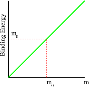
In order to facilitate a theoretical treatment, we construct simplified models of the recombination and selection steps. Let us describe the selection step first. For selection, we need a model that connects genotype and phenotype, which is in this case the binding energy of the DNA to the protein, as well as a model that specifies selection on the phenotype. We adopt the simplest relationship between genotype and phenotype. We assume that each nucleotide contributes to the binding energy independently and additively. Each nucleotide can be one of the ${\mathcal{A}}$($=4$) nucleotides (representing A, C, G and T), among which one is favorable and the rest are equally deleterious. For simplicity, we denote the contribution of a specific site to the binding energy $1$ ($0$) if therein sits a favorable (deleterious) nucleotide. We will refer to a favorable (deleterious) nucleotide as a match (mismatch) with respect to the optimal sequence. This formulation can be derived from a two-state model for protein-DNA binding (VON HIPPEL and BERG $1986$; GERLAND and HWA $2002$). The binding energy of the sequence is simply the number of sites with favorable nucleotides.

Fig. (1a) shows schematically the shape of our phenotypic landscape. Of course, our model reflects just this simplest possibility. In reality, the phenotypic landscape could be much more complicated and is rarely known; in fact, a significant advantage of directed evolution over rational design is that this kind of knowledge is not necessary (e.g. ARNOLD $2001$). Our strategy here is to study the simplest non-trivial model available, obtain a thorough understanding, with the hope of proceeding to more complicated situations to see which results obtained in the simple model are general and which are model specific. Having specified the phenotypic landscape, we next describe the selection protocol. Selection acts on the binding energy of the sequences. As noted above, in (molecular) breeding, truncation selection is used. We define the selection strength via the fraction $\phi$ of selected members of the total population. Suppose we have a distribution of population $P_{{m}}$ in terms of the binding energy ${m}({m}=0,1,\ldots,L)$, where $L$ is the total number of active sites. The threshold ${{m}_{0}}$ is self-consistently determined by

$$\phi=\alpha P_{{{m}_{0}}}+\sum_{{m}={{m}_{0}}+1}^{L}P_{{m}},$$ (1)

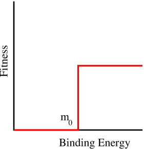
where $\alpha$ in the first term takes into account of the partial selection on the threshold state ${{m}_{0}}$. $\phi$ varies from $\phi\lesssim 1$ (relatively weak selection) to small $\phi$ (relatively strong selection). For those sequences whose number of matches are above (below) ${{m}_{0}}$, their fitness is $1$ ($0$), and they are selected (discarded) [see Fig. (1b)]. In the truncation selection scheme every member’s fitness is collectively and dynamically determined by both the phenotypic distribution of the population $P_{{m}}$ and selection strength $\phi$. In contrast, most fitness landscapes studied prescribe for each genotype a preset fitness value and its effective fitness value is simply its own fitness over the mean fitness (CROW and KIMURA $1970$). Truncation selection generates correlations (i.e., linkage) between loci, hence it is epistatic (OTTO and BARTON $2001$; SHNOL and KONDRASHOV $1993$).

We note in passing that the term truncation selection has also been used to mean a fixed step-like landscape. In population genetics literatures, a fixed step-like landscape is also called hard truncation selection, and the selection scheme we employed is sometimes termed soft truncation selection. Due to the dynamical nature of the selection scheme, using fitness as a yardstick for the evolution is not very useful; for example, the mean fitness of the population is always $\phi$ by definition. As a consequence, we will focus on the evolution of the phenotypic distribution, i.e., the distribution of binding energies, instead of the fitness distribution.

We now turn to the discussion of recombination. Our basic approach here will be to make a substantial simplification of the actual situation and assume perfect recombination between all nucleotides. Namely, in building each new sequence after selection, each nucleotide independently samples the nucleotides at the corresponding sites in the entire selected population. Formally, this amounts to assuming that the fragmentation and reassembly process is repeated often enough such that there is no linkage between any of the nucleotides. This is undoubtedly false in detail for the experiments done to date, but we shall see that this approximation is quite good for describing the result of a scenario involving the more feasible case of a finite number of crossovers. The advantage of this “maximal” recombination is that it allows for an analytic solution of the model, as will be presented in the remainder of this paper. Finally, we assume simple point mutation for each site. Namely, each nucleotide is independently subject to mutation rate ${\mu_{0}}$ per generation. This process includes both beneficial and deleterious mutations.

Figure 2: Maximal recombination under a general interpretation. Each line represents a DNA sequence. Crosses represents active sites with variable length fixed regions in between. Crosses with different background patterns represent different phenotypes for active sites. In building a new sequence, each active site independently samples the corresponding sites in the entire selected population.

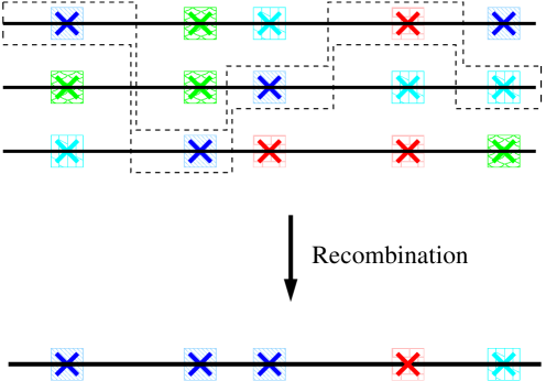
It is worth pointing out that our approach to recombination may have more general applicability than merely as an approximation for the DNA binding problem. In many cases of DNA shuffling, the initial library of genes coding for an interesting protein is chosen from closely related species so as to ensure proven functionality and sufficient homology to allow recombination. Let us imagine that the majority of the nucleotides along those DNA sequences are already optimal, and (non-synonymous) mutations of these nucleotides are lethal. Hence, we can consider these nucleotides to be fixed during the entire evolutionary process and ignore them except insofar as they provide enough homology so that overlapping single-stranded fragments from different DNA sequences can anneal with each other (and do not anneal with other fragments by accident) during the self-primed PCR re-assembly step (STEMMER $1994$a; $1994$b) . For the remaining active sites, we assume that they are (a)  far enough from each other so that recombination happens freely between any two; (b) they are subject to point mutations with rate ${\mu_{0}}$ per nucleotide per generation. Therefore, each active site, along with its fixed flanking homologous regions (whose size or exact delineation do not matter), constitutes a segment. To build a new sequence from recombination, a number of overlapping fragments (which when put together cover the entire sequence) are assembled, with each fragment obtained from randomly sampling the corresponding fragments (i.e., having the same active site) in the selected population. This idea is depicted in Fig. (2) and is an exact realization of our maximal recombination model. Of course, one has to be careful to intersperse an experimental selection step that will eliminate all lethal variants (due to mutation) before proceeding to an actual selection based on useful variation. To proceed, we would then have to explicitly take into account the transformation from gene sequence to amino acid, as the selection would be on the basis of some desired activity of the protein. We do not pursue this line of investigation any further in this work.

Finally, we can rephrase our model in terms of the standard language of population genetics. Each site can be referred to as a locus, which can have ${\mathcal{A}}$ alleles, one favorable (match) and the rest (mismatches) equally unfavorable. The set of all $L$ loci form a chromosome. The recombination scheme is such that the allele of each locus of every new chromosome is chosen by randomly sampling the alleles at the corresponding locus of all the selected chromosomes. The fitness value of each chromosome is either $1$ ($0$), when the number of matches it has is above (below) the threshold $m_{0}$. For clarity, we list the correspondence in Table 1.

DNA-protein binding	Population Genetics
DNA sequence	chromosome
nucleotide	locus
binding energy	phenotypic value:matches
selection via binding to protein	dynamical truncation selection

Table 1: The correspondence between two languages: directed molecular evolution and population genetics.

In genetic algorithms and evolutionary strategies, a research area in computer science where the principles of evolution are employed to find optimal solutions to complex problems (BEYER $2001$), a similar setting has been investigated by Mühlenbein and Schlierkamp-Voosen ($1993$), mostly via computer simulation. Various aspects of classical breeding have also been studied in population genetics (CROW and KIMURA $1970$). Kimura and Crow investigated the response of individual loci to selection in one round, under linkage-free condition (CROW and KIMURA $1970$; KIMURA and CROW $1978$). Kondrashov ($1995$) studied a model with a different type of dynamical fitness landscape, where the fitness value of a genotype depends only on the difference between its phenotypic value and the mean of the phenotypic distribution, in units of variance of the phenotypic distribution. Along with the assumption of deleterious mutations, conventional recombination, and a Gaussian distribution before selection (which, as we shall see, is in fact equivalent to using maximal recombination), he derived evolutionary recursion relations and obtained analytical expressions that characterize the equilibrium position. We shall make connections with these works in appropriate places.

RESULTS

Dynamics of maximal recombination
To summarize the above discussion, in the language of population genetics which we will adopt from here on, we have a haploid population of $N$ chromosomes each with $L$ loci, and we study the evolution with dynamical truncation selection, maximal recombination and point mutation as specified above. We fix the order of operation to be selection, recombination and mutation. At each step the population size $N$ is kept constant. 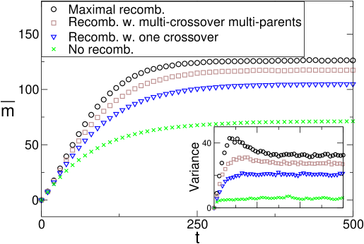This model is easily simulated on a computer. Fig. (3) shows simulation results for evolutionary trajectories of the average and variance of the match distribution under weak selection. For comparison, we show results from four different evolutionary protocols: no recombination; single random crossover; multiple crossovers and multiple parents (which is the situation closest to experiments); and maximal recombination. It is evident that recombination improves both the dynamics and equilibrium state as compared to the case with no recombination. For our phenotypic landscape and selection scheme, the more recombination the better. Furthermore, the maximal recombination scheme captures the essential effect of recombination and provides a reasonable approximation to the more readily achievable case of multiple crossovers from multiple parents. In the alternative case of strong selection (not shown), all evolutionary protocols propel the population to an equilibrium state very close to the optimal state; however the population reaches the equilibrium state much faster when recombination is applied.

Figure 3: Comparison of evolutionary trajectories for four different evolutionary protocols under weak selection. Shown are simulation results of the evolutionary trajectory of the average number of matches ${\overline{m}}$ for the population, with an initial clonal population with no matches at any chromosomes. x: no recombination; Triangle: recombination with one random crossover; Square: recombination with multiple crossover and multiple parents, using a per bond crossover probability of $0.025$. Circle: maximal recombination. Shown in the inset are the corresponding variances of the distributions versus time, ordered in the same way as the matches vs. generations curves. Here sequence length $L=170$, selection strength $\phi=.9$, mutation rate ${\mu_{0}}=.01$ and population size $N=10^{4}$.

In our analytical work we will assume, unless specifically noted otherwise, the population size $N$ to be very large so that random genetic drift is negligible; we will briefly discuss finite size effects at the end. We focus on the evolution of such macroscopic characteristics of the population as mean and variance, as opposed to “microscopic” properties such as the fate of individual mutations. As already noted, the fitness distribution itself does not describe the evolution. We instead study the evolution of the phenotypic (match) distribution, focusing on its first and second moments. For simplicity we assume linkage equilibrium at the beginning of evolution. This is in fact not a stringent assumption, since linkage equilibrium is achieved anyway right after one round of recombination.

Even before going into any details of the analysis, it is not difficult to understand why recombination is highly beneficial in this model. Selection, as it operates on the phenotype, which in this case is the total number of matches, introduces linkage. After the selection step, recombination immediately restores total linkage equilibrium. resulting into a broader distribution [see Fig. (3) inset]. A broader distribution means better response to subsequent selection and hence faster evolution. The following analysis describes how this works in a fully quantitative way, in the maximal recombination model.

Dynamics without mutation: We start from the simplest case where the mutation rate ${\mu_{0}}$ is set to be $0$. We assume that each locus has the same binary distribution characterized by the probability of being favorable (i.e., a match) ${p}(0)$ $(\neq 0)$. This is in fact the case most relevant to the DNA shuffling experiments to date, where ${\mu_{0}}$ is kept extremely small and the diversity is almost entirely provided by the diversity which existed in the initial library (KURTZMAN et.al. $2001$). Starting from the homogeneous initial condition, we expect that every locus follows the same evolution trajectory, as the evolution dynamics preserve permutation symmetry of different loci. With this in mind, we focus on the evolution of the probability ${p}(t)$ for one locus to be favorable at the end of generation $t$. The phenotypic probability distribution for the number of matches of a chromosome at the end of round $t$ is then a binomial distribution characterized by mean $L{p}(t)$. Assuming that $L$ is large (For a more accurate treatment without the assumption of large $L$, see Appendix B), the binomial distribution is well approximated by a Gaussian distribution $P(m,t)$ :

$$P(m,t) = \frac{1}{\sqrt{2\pi\sigma^{2}(t)}}\exp\left(-\frac{(m-{\overline{{m}}}(t))^{2}}{2\sigma^{2}(t)}\right)$$ (2)

$${\overline{{m}}}(t) = L{p}(t)$$ (3)

$$\sigma^{2}(t) = L{p}(t)\,(1-{p}(t))$$ (4)

Given such a distribution at the end of generation $t$, we now discuss step by step the effects on the distribution due to various operations in the evolutionary protocol. In generation $t+1$, selection cuts out the low $m$ tail of the Gaussian distribution. It is straightforward to calculate that the mean match number of the selected population ${\overline{{m}}}_{\textrm{s}}$ is

$${\overline{{m}}}\rightarrow{\overline{{m}}}_{\textrm{s}}={\overline{{m}}}+\sigma G(\phi).$$ (5)

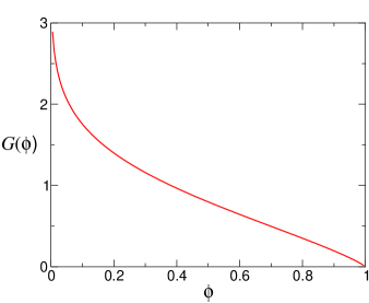
The new mean can thus be expressed as the old mean plus an improvement due to selection, which is simply the product of the old standard deviation and a factor $G(\phi)$ that solely encodes the strength of selection. Here $G(\phi)$ is the mean for the normalized distribution resulting from a standard Gaussian distribution truncated by a $1-\phi$ fraction taken off the tail, namely

$$G(\phi)=\frac{1}{\sqrt{2\pi}\phi}\exp\left(-\frac{1}{2}X(\phi)^{2}\right),$$ (6)

where $X(\phi)$ is the match threshold defined through

$$\phi=\int_{X(\phi)}^{\infty}\frac{dx}{\sqrt{2\pi}}\exp\left(-\frac{1}{2}x^{2}\right).$$ (7)

Fig. (4) shows the behavior of $G(\phi)$. For $0.3<\phi<1$, $G(\phi)$ is approximately a linear function of $\phi$ (with slope roughly $-1.5$), and $G(\phi)\rightarrow(1-\phi)\sqrt{2\ln\,(1-\phi)^{-1}}$ as $\phi\to 1$. In the strong selection limit, i.e., $\phi\rightarrow 0$, $G(\phi)\rightarrow\sqrt{2\ln\phi^{-1}}$, which diverges.

Figure 4: The selection factor $G(\phi)$. $G(\phi)$ diverges at strong selection $\phi\to 0$ and goes to zero at weak selection $\phi\to 1$.

After selection, the recombination step restores the independence of each locus. The population distribution of matches returns to a binomial (Gaussian) distribution characterized by mean ${\overline{{m}}}_{\textrm{s}}$.

$${\overline{{m}}}_{\textrm{r}} = {\overline{{m}}}_{\textrm{s}}$$ (8)

$$\sigma_{\textrm{r}}^{2} = {\overline{{m}}}_{\textrm{r}}(1-{\overline{{m}}}_{\textrm{r}}/L)$$ (9)

Because of the independence of each locus, we can reexpress Eq. (8) in terms of individual match probability ${p}_{\textrm{r}}$ and ${p}(t)$:

$${p}_{\textrm{r}}={p}(t)+\frac{\sqrt{{p}(t)(1-{p}(t))}}{\sqrt{L}}G(\phi),$$ (10)

and the variance of the distribution is simply $L{p}_{\textrm{r}}(1-{p}_{\textrm{r}})$. Eq. (10) has two features: First, the scaled combination of ${G(\phi)}/{\sqrt{L}}$ is the single control parameter. Second, the change of ${p}$ is proportional to the square root of the variance, instead of the variance itself as in the case of a fixed landscape (CROW and KIMURA $1970$). This results in a slower evolution for populations that are in the middle of the landscape, but results in a speed-up near the ${p}=0$ and ${p}=1$ absorbing states.

In the case of weak selection, Eq. (10) can be approximated by its continuous-time version:

$$\frac{d{p}}{dt}=\frac{G(\phi)}{{\sqrt{L}}}\sqrt{{p}(1-{p})}.$$ (11)

The evolutionary dynamics is governed by two fixed points: ${p}=0$ and ${p}=1$. ${p}=0$ is a trivial unstable fixed point. When ${p}(0)>0$, the population moves toward ${p}=1$ with following time dependence,

$${p}(t)=\frac{1}{2}\left[1-\sin(\beta-\frac{G(\phi)}{{\sqrt{L}}}t)\right],$$ (12)

where $\beta=\sin^{-1}(1-2{p}_{0})$. Eq. (11) and its solution have also been derived in Mühlenbein and Schlierkamp-Voosen ($1993$). From this we see that the system actually reaches the optimal state in a finite time $T$, rather that approaching exponentially. This is due to the square-root behavior of the velocity near ${p}=1$ noted above. $T$ is given by

$$T=(\frac{\pi}{2}+\beta)\frac{{\sqrt{L}}}{G(\phi)}.$$ (13)

A surprising feature of this result is that $T$ is finite even in the limit of ${p}(0)\rightarrow 0$, i.e., a random initial population that has an arbitrarily small chance of having matches in its chromosomes. Hence, the maximum amount of time $T_{\textit{m}ax}$ the population needs to converge to the optimum is

$$T_{\textit{m}ax}={\pi}\frac{{\sqrt{L}}}{G(\phi)}.$$ (14)

To appreciate this result and the benefit of recombination, it is helpful to compare it with that of pure enrichment (i.e., selection only), given the same initial condition. Starting from ${p}(0)$, the population distribution initially is a binomial distribution. Selection keeps chopping off the low tail of this distribution round by round, and stops when the distribution contains only the perfect state with $L$ matches. Note that since here we care about the extreme tail of the distribution, the Gaussian approximation is no longer adequate. Based on this scenario, the evolution time $T$ is determined by the overall fraction of the population remaining after $T$ rounds, $\phi^{T}$, which must be the fraction starting out in the perfect state, ${p}(0)^{L}$. Therefore,

$${T}={L}\frac{\ln\,{p}(0)}{\ln\phi},$$ (15)

which diverges when ${p}(0)\rightarrow 0$. This divergence can be understood as a result of the initial distribution becoming both closer to $0$ and narrower in width as ${p}(0)\rightarrow 0$. This behavior is dramatically different from that for the recombination case shown in Eq. (14). Comparing Eq. (15) with Eq. (13), we see another significant difference. The evolution time scales differently with $L$ in the two cases; as $\sqrt{L}$ in the case of recombination and as $L$ in the case of enrichment. This means that the longer the chromosome, the greater the benefit of recombination.

We have shown that recombination provides a significant improvement when ${p}(0)$ is very small. In general, it can be seen by comparing Eq. (15) with Eq. (13) that under the conditions when the evolution takes a longer time [i.e, the worse the initial condition, the weaker the selection strength (larger $\phi$) or the longer the chromosome], recombination is highly beneficial. Under the opposite conditions, recombination is usually still not worse. There are cases where recombination does not confer any benefit, for example if the selection strength is so strong that the selected population all belongs to the optimal state. However, when ${p}(0)$ is very close to one, recombination actually takes longer, since $T$ vanishes linearly in $1-{p}(0)$ without recombination, and as a square-root, $\sqrt{1-{p}(0)}$ with. We shall encounter a similar phenomenon when we discuss the equilibrium state. The reason for this is that recombination repopulates all the states, whereas pure enrichment does not. Since for $p(0)$ very close to 1, the best state is the most highly populated, recombination can only hurt. Again we must note in passing that in the case of very strong selection, the results from our continuum treatment deviate from those of the actual discrete process.

Dynamics with homogeneous initial condition: So far, we have studied the dynamics of maximal recombination in the absence of mutation. Now we insert the point mutation process into the evolutionary dynamics. As a first step, we again assume a homogeneous initial condition such that each locus has the same probability of being favorable (i.e., a match) ${p}(0)(\neq 0)$. Mutation is the final step of the round. Since we only consider single base mutations, linkage is not introduced in the process. The mutation process we consider here includes both forward and back mutations; by itself, it drives the chromosomes toward the maximum entropy point $L/{\mathcal{A}}$ (or $1/{\mathcal{A}}$ in terms of ${p}$), which is in general opposite to the direction of selection. A simple calculation yields

$${{p}}_{\textrm{{m}}}={{p}}_{\textrm{r}}+\frac{{\mu_{0}}}{{\mathcal{A}}-1}(1-{\mathcal{A}}{{p}}_{\textrm{r}})$$ (16)

Combining this equation with Eq. (10), we obtain a recursion relation for the evolution of ${p}$:

$${{p}}(t+1)={{p}}(t)+\frac{{\mu_{0}}}{{\mathcal{A}}-1}(1-{\mathcal{A}}{{p}}(t))+\frac{G(\phi)}{\sqrt{L}}\sqrt{{{p}}(t)\left(1-{{p}}(t)\right)},$$ (17)

where we have dropped a correction factor $(1+{\mu_{0}}{\mathcal{A}}/({\mathcal{A}}-1))$ in the last term, since ${\mu_{0}}\ll 1$. It is clear that the second term on the right hand side of the recursion relation is due to mutation, and the third term to selection and recombination. When the third term dominates the second term, the dynamics is essentially the same as that with no mutation as discussed above. When ${p}>1/{\mathcal{A}}$, the mutational contribution becomes harmful to the evolution.

The recursion relation Eq. (17) has an interesting feature. If we divide Eq. (17) by ${\mu_{0}}$ on both side, we have

$$\frac{{{p}}(t+1)-{{p}}(t)}{{\mu_{0}}}=\frac{1}{{\mathcal{A}}-1}(1-{\mathcal{A}}{{p}}(t))+\frac{G(\phi)}{{\mu_{0}}\sqrt{L}}\sqrt{{{p}}(t)\left(1-{{p}}(t)\right)}.$$ (18)

Eq. (18) says that the scaled combination ${G(\phi)}/({\mu_{0}}\sqrt{L})$ is the single control parameter (as opposed to ${G(\phi)}/{\sqrt{L}}$ in the case of no mutation). In other words, if different choices of parameters result in the same combination ${G(\phi)}/({{\mu_{0}}\sqrt{L}})$, the corresponding dynamics are exactly the same as long as the time scale in each case is rescaled by its respective mutation rate ${\mu_{0}}$. Note that in Eq. (17) or Eq. (18), ${p}(t)$ can go above $1$ when selection is strong; this unrealistic result comes from the Gaussian approximation to the population distribution that becomes inaccurate when the population reaches the neighborhood of the optimal state. We will further address the error due to the Gaussian approximation in our discussion of the equilibrium state.

Figure 5: Comparison of simulation results and theory. The evolutionary trajectories of three simulations with totally different parameters [but same scaling variable ${G(\phi)}/({{\mu_{0}}\sqrt{L}})$] collapse into a single curve when time is properly rescaled, and this curve agrees well with the theoretical result obtained from Eq. (17). Here the three simulations all start from a homogeneous initial condition of ${p}(0)=0.1$ and population size $N=10^{4}$.

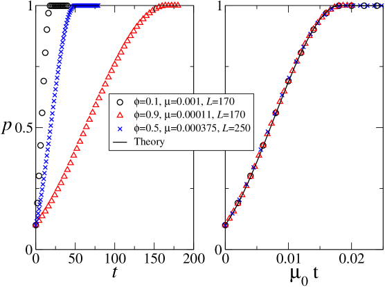
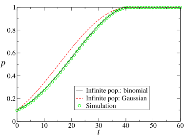
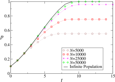
As a test of our theory, Fig. (5) shows that the theoretical predictions, including the scaling with $G(\phi)/({\mu_{0}}\sqrt{L})$, agree extremely well with simulation data. This indicates that the finite-population effect in this landscape is insignificant, and the Gaussian approximation to the binomial distribution is appropriate for sequences of long length $L$.

When selection is weak so that the change in ${p}$ in each round is small, the evolution equation (17) can again be accurately approximated by its continuous time version,

$$\frac{d{p}}{dt^{\prime}}=(1-{\mathcal{A}}{p})+C\sqrt{{p}(1-{p})},$$ (19)

where $t^{\prime}\equiv({\mu_{0}}/({\mathcal{A}}-1))\,t$ and $C\equiv({\mathcal{A}}-1)G(\phi)/({\mu_{0}}\sqrt{L})$. The explicit solution of this equation can be found in Appendix A.

An explicit analytical comparison of the evolutionary performance between the evolutionary protocol with and without recombination is not available. Both recombination and mutation can serve to generate diversity, but the greater benefit of recombination is due to that facts that (a) recombination breaks up the linkage introduced by selection much more effectively than mutation does; breaking of linkage helps broaden the distribution (as selection narrows the distribution) and in turn facilitates more efficient future selection, hence speeding up the evolution, and (b) recombination keeps the mean of the population unchanged, whereas mutation goes against selection (once the population goes beyond the maximum entropy point). Therefore, as has been recognized for a long time, recombination is able to generate variety without the excessive baggage of deleterious mutations.

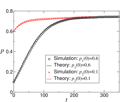
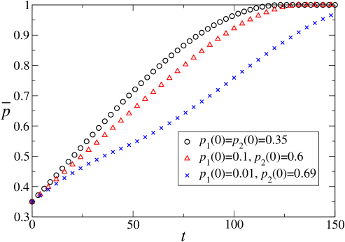
Dynamics with inhomogeneous initial condition: In the previous discussion, we assumed a simple homogeneous initial condition. An immediate question concerns what happens with a inhomogeneous initial condition, i.e. would different loci synchronize with each other after a short transient period or would they go their separate ways and only meet at the end of the process? To answer this question, we choose a linkage-free initial condition where half of the loci have probability ${p}_{1}(0)$ of being a match, and the other half have probability ${p}_{2}(0)$ of being a match. Assuming again that $L\gg 1$, a similar derivation to the one presented above produces

$${p}_{1}(t+1) = {p}_{1}(t)+\frac{{\mu_{0}}(1-{\mathcal{A}}{p}_{1}(t))}{{\mathcal{A}}-1}+\frac{G(\phi)}{\sqrt{L/2}}\frac{{{p}}_{1}(t)(1-{{p}}_{1}(t))}{\sqrt{{{p}}_{1}(t)(1-{{p}}_{1}(t))+{{p}}_{2}(t)(1-{{p}}_{2}(t))}}$$

$${p}_{2}(t+1) = {p}_{2}(t)+\frac{{\mu_{0}}(1-{\mathcal{A}}{p}_{2}(t))}{{\mathcal{A}}-1}+\frac{G(\phi)}{\sqrt{L/2}}\frac{{{p}}_{2}(t)(1-{{p}}_{2}(t))}{\sqrt{{{p}}_{1}(t)(1-{{p}}_{1}(t))+{{p}}_{2}(t)(1-{{p}}_{2}(t))}}$$ (20)

Fig. (6) compares these results with a evolutionary trajectory with inhomogeneous initial conditions. It is clear that different locus go their own ways.

Figure 6: Evolution of individual match probability ${p}$ with inhomogeneous initial condition. The initial condition is chosen so that half of the loci have initial match probability of ${p}_{1}(0)=.1$, while the remaining half has ${p}_{2}(0)=.6$. The two simulation curves track the two different groups of loci. The solid curves are theoretical results from Eq. (20). Simulations use the following parameters: $L=170$, $\phi=.9$, ${\mu_{0}}=.01$ and $N=10^{4}$.

If mutation is ignored, one find that the relative changes in the individual match probabilities are

$$\frac{{p}_{1}(t+1)-{p}_{1}(t)}{{p}_{2}(t+1)-{p}_{2}(t)}=\frac{{p}_{1}(t)(1-{p}_{1}(t))}{{p}_{2}(t)(1-{p}_{2}(t))},$$ (21)

i.e., proportional to the ratio of the variance on each locus. In other words, the selection works on variance; different locus with different ${p}$ experience different selection pressures depending on their contribution to variance. This means that in the case of inhomogeneous initial conditions, the evolution process will be dominated by whichever loci have very small initial ${p}(0)$; see Fig. (7) for an explicit demonstration of this conclusion.

Figure 7: Comparison of simulation results for the average individual match probability $\overline{p}$ for different initial conditions, in the absence of mutation. $\overline{p}$ is the individual match probability ${p}$ averaged over loci. Here $L=170$, $\phi=.9$ and $N=10^{4}$.

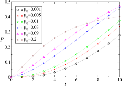
Dynamics with clonal initial condition: In the above theoretical analysis we have assumed an initial condition which already has all the favorable alleles available in the population, and mutation was relatively unimportant. In many situations, mutations are absolutely necessary for the system to find the optimal state. This scenario could happen for a system prepared with a clone-like initial condition with some loci lacking the beneficial alleles. In this section we focus on this case and study the effect of different mutation rates on the evolutionary dynamics. We start from the simplest case which is a clonal initial condition with no beneficial allele at any locus (i.e., ${p}(0)=0$). For this simple case, the obviously best strategy is to subject the system to maximal mutation rate ${\mu_{0}}=({\mathcal{A}}-1)/{\mathcal{A}}$ until the system reaches ${p}=1/{\mathcal{A}}$, and then to stop mutation altogether. However, this naive strategy does not apply to other clonal initial conditions which are inhomogeneous; here it is not a priori clear when one should turn off mutation, since we have access only to measurements of the full phenotype.

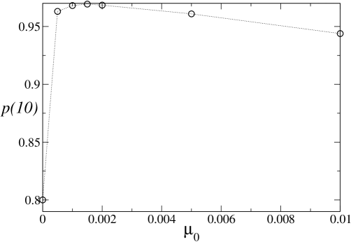
Assuming that mutation rate is fixed, we can gauge the performance of different choices of mutation rate by measuring ${p}$ after a given number of generations. Fig. (8) shows a comparison of simulations starting at ${p}(0)=0$ with different mutation rate using this criterion. It is clear that there is a “optimal” mutation rate. Of course, the ”optimal” mutation rate depends when evolution is terminated.

Figure 8: Simulation results of different mutation rates given a clone initial condition of ${p}(0)=0$. (a) Evolutionary trajectories for different choices of mutation rate ${\mu_{0}}$. (b) Comparison of individual match probability at the tenth generation ${p}(10)$ for different mutation rates. The ”optimal” mutation rate is around ${\mu_{0}}=.08$ under this condition. Here $L=170$, $\phi=.1$ and $N=10^{4}$.

In the more common situation, a majority of the loci are already occupied by beneficial alleles, and for the rest, mutation is required to create the beneficial allele. In this case as well, we can see the existence of an “optimal” mutation rate, as in Fig. (9).

Figure 9: Simulation results for different mutation rates given an inhomogeneous clonal initial condition. Initially, all the member of the population have the same haplotype; $1/5$ of the loci are occupied by mismatches and the rest by matches. Here $L=170$, $\phi=.1$ and $N=5\times 10^{5}$.

In conclusion, mutation is necessary when there is limited diversity in the initial library. Even in this case, mutation is only helpful in the short term dynamics, but harmful to the equilibrium state. In a realistic experiment, since breeding usually proceeds for a only few generations there would exist an “optimal” mutation rate.

Equilibrium state of maximal recombination: Having studied the dynamical behavior of the model in the previous sections, we now turn to the study of its equilibrium properties, focusing on the mean number of matches in equilibrium. This quantity plays the role here that genetic load does in normal evolution problems. Strictly speaking, genetic load is the difference in fitness between the equilibrium population and the optimal fitness state. In our case, the optimal state has fitness value $1$, and the mean fitness of the population is simply $\phi$, so the difference is trivially $1-\phi$. However, since the purpose of the experiments is to maximize the phenotypic value, i.e., the number of matches, the mean number of matches is a reasonable way to characterize the equilibrium state, and the “cost” of mutations. Going back to the language of DNA protein binding, what we are using to characterize the equilibrium is the mean binding affinity of the DNA sequence.

Under the Gaussian approximation, the equilibrium value ${\hat{{p}}}$ can be found by setting ${p}(t+1)={p}(t)$ in Eq.( 17), yielding

$$\frac{{\hat{{p}}}(1-{\hat{{p}}})}{({\mathcal{A}}{\hat{{p}}}-1)^{2}}=\frac{1}{({\mathcal{A}}-1)^{2}}\left(\frac{{\mu_{0}}\sqrt{L}}{G(\phi)}\right)^{2}$$ (22)

Figure 10: Equilibrium value of individual match probability ${p}$ as function of ${{\mu_{0}}\sqrt{L}}/{G(\phi)}$. The $y=x^{2}$ curve denotes the asymptotic behavior of ${p}$ in strong selection (low mutation) resulting from the Gaussian approximation, Eq. (24). For simulation results: $L=170$, ${\mu_{0}}=.01$, $N=10^{4}$.

As shown in Fig. (10), for weak and intermediate selection strength this result agrees with the simulation data. For the parameter regime of strong selection (or very small mutation rate), ${{\mu_{0}}\sqrt{L}}/{G(\phi)}$ is no longer a good scaling variable, and the Gaussian approximation begins to deviate from the exact result.

For weak selection (i.e., $({{\mu_{0}}\sqrt{L}}/{G(\phi)})^{2}\gg 1$) the equilibrium probability is near $1/{\mathcal{A}}$. We have

$${\hat{{p}}}-\frac{1}{{\mathcal{A}}}=\frac{({\mathcal{A}}-1)^{\frac{3}{2}}}{{\mathcal{A}}^{2}}\frac{G(\phi)}{{\mu_{0}}\sqrt{L}}$$ (23)

When selection is relatively strong, i.e., when $({{\mu_{0}}\sqrt{L}}/{G(\phi)})^{2}\ll 1$, the equilibrium position is

$$1-{\hat{{p}}}=\left(\frac{{\mu_{0}}\sqrt{L}}{G(\phi)}\right)^{2}$$ (24)

As shown in Fig. (10), for the parameters employed there, this power law is accurate in the region of $0.1\leq({{\mu_{0}}\sqrt{L}}/{G(\phi)})^{2}\leq 1$. ( A more precise statement about the lower cutoff for the validity of Eq. (24) is ${\mu_{0}}L>\ln\,\phi^{-1}$; see discussion below). This ${\mu_{0}}^{2}$ dependence has also been derived by Kondrashov ($1995$) for a different type of dynamical selection scheme.

It is well know that in a fixed smooth landscape, the mutational load is ${\mu_{0}}L$ in the strong selection limit. We see from the above that for our breeding problem, strong selection, at least in the Gaussian approximation, produces a load that scales with ${\mu_{0}}^{2}$ rather than the usual ${\mu_{0}}$. The reason for this scaling is easy to understand: With recombination, the change due to selection of ${p}L$, the number of matches, is proportional to the width of the distribution $\sqrt{L{p}(1-{p})}\approx\sqrt{L(1-{p})}$ (which is independent of the Gaussian approximation), and mutation reduces ${p}L$ by $-{\mu_{0}}L$. Balancing the two effects we arrive at the ${\mu_{0}}^{2}$ scaling. This simple argument shows that the ${\mu_{0}}^{2}$ law is a generic result for the genetic load when recombination is at work (which happens whenever the selected population still occupies a number of different states). When selection strength is sufficiently strong that the selected population lies almost entirely in the optimal state, recombination becomes ineffective as there is no diversity within the selected population. As a result [as shown in Fig. (10)], the Gaussian result is no longer valid. In fact, as we shall show below, in this case the usual mutational load of O(${\mu_{0}}$) takes over.

For small mutation rates, as we shall see, the mean mismatch number is small at equilibrium, except for very weak selection. This is in contradistinction to the dynamic case, where we focused on the case where there were a large number (order $L$) of initial mismatches. There, for most of the time, the Gaussian approximation is quite adequate. In equilibrium, however, this is generically not the case, and a more careful treatment is warranted.

To study this issue in more detail, we can make use of a more powerful approximation scheme that accurately covers both the strong selection and extremely strong selection cases so as to find the equilibrium position. Since $L{p}\sim L$, we shift our focus to the mismatch probability ${q}\equiv 1-{p}\sim 0$, and, before selection, the population distribution in terms of mismatch should follow a Poisson distribution $P_{k}=\mathcal{Q}^{k}e^{-\mathcal{Q}}/{k!}$, where $\mathcal{Q}\equiv L{q}$. Call $C_{k_{0}}$ the cumulative probability of being in a state with $k\leq{k_{0}}$. Selection results in

$$\phi=C_{k_{0}-1}+\alpha P_{k_{0}},$$ (25)

where $k_{0}$ is the threshold, which is determined by the condition that $C_{k_{0}-1}<\phi\leq C_{k_{0}}$. $\alpha\leq 1$ counts the partial selection on the members of population with $k_{0}$ mismatches.

The result of selection, recombination and mutation are

$${q}_{\textrm{r}} = \frac{1}{L\phi}\left(\sum_{k=0}^{k_{0}-1}kP_{k}+\alpha k_{0}P_{k_{0}}\right),$$ (26)

$${q}_{\textrm{{m}}} = {q}_{\textrm{r}}+{\mu_{0}}-\frac{{\mathcal{A}}}{{\mathcal{A}}-1}{\mu_{0}}{q}_{\textrm{r}},$$ (27)

where ${q}_{\textrm{r}}$ (${q}_{\textrm{{m}}}$) is the individual mismatch probability right after recombination (mutation). The last term is negligible as it arises from extremely rare compensatory beneficial mutations. Combining Eqs. (25, 26, 27), we arrive at the following equation that determines the equilibrium average mismatch number $\mathcal{\hat{Q}}$:

$$\phi=\frac{e^{-\mathcal{\hat{Q}}}}{k_{0}+{U}-\mathcal{\hat{Q}}}\sum_{k=0}^{k_{0}-1}\frac{k_{0}-k}{k!}{\mathcal{\hat{Q}}}^{k},$$ (28)

where ${U}\equiv{\mu_{0}}L$ is the genomic mutation rate. The physical $\mathcal{\hat{Q}}(\phi)$ curve is given by the envelope of the various ${\hat{{q}}}(\phi,k_{0})$ for different $k_{0}$’s, and is piecewise analytic. Fig. (11) shows the difference between this solution and the solution given by the Gaussian approximation. Even though the Gaussian approximation has generally the right trend, for this small mutation rate the Gaussian approximation is numerically off by a large percentage, except for extremely weak selection. Also, for $\phi<e^{-{U}}$, selection only preserves the optimal state at equilibrium, recombination stops working, and Eq. (28) produces $\mathcal{\hat{Q}}=L-L{\hat{{p}}}={U}$, the conventional mutational load, which is the result that is unobtainable from the Gaussian approximation.

Figure 11: Theoretical evaluation of equilibrium value of mean mismatches: comparison of Gaussian approximation and Poisson approximation. Curves corresponding to different $k_{0}$ values are trial solutions of Eq. (28) with different choices of threshold $k_{0}$. The envelop of the trial solutions is the physical solution. For comparison, the solution given by Gaussian approximation is also plotted. Here $L=170$, ${\mu_{0}}=.001$.

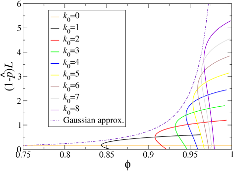
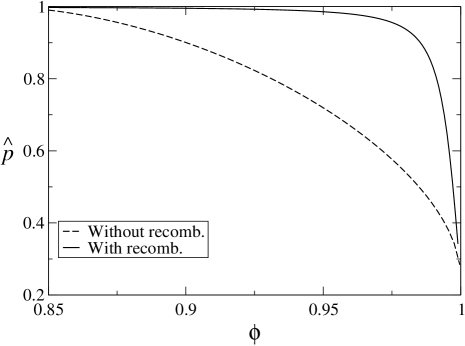
Now we come back to the question of how much of an improvement is conferred by recombination. The easiest way to approach the question is through a graph, Fig. (12), directly comparing the equilibrium state with and without recombination, for the same value of ${\mu_{0}}$. To do this, we use the analysis for the no recombination case from Cohen and Kessler ($2003$):

$$-\frac{\ln\phi}{{U}}=\frac{1}{{\mathcal{A}}-1}+\frac{{\mathcal{A}}-2}{{\mathcal{A}}-1}{\hat{{p}}}_{\rm A}-\sqrt{\frac{4}{{\mathcal{A}}-1}{\hat{{p}}}_{\rm A}(1-{\hat{{p}}}_{\rm A})}.$$ (29)

Here ${\hat{{p}}}_{\rm A}$ denotes the equilibrium value of total number of matches divided by chromosome length $L$ for the no-recombination case. The first thing to notice is that at the two extreme limits of maximal selection and no selection, the two approaches yield the same result. The curves are nevertheless very different. In order to understand this difference better, we first focus on the case of intermediate selection. We re-express Eq. (24) to simplify the comparison with Eq. (29). Using the small $\phi$ limit of $G$, we obtain

$$-\frac{\ln\phi}{{U}}=\frac{{\mu_{0}}}{2(1-{\hat{{p}}})}$$ (30)

Without recombination, ${\hat{{p}}}$ is an order $1$ function of $\chi\equiv-\ln\phi/{U}$, whereas with recombination, the relation involves ${\mu_{0}}$ as well as $\chi$. Thus, with recombination, the only way $\chi$ can be of order 1 is if $1-{\hat{{p}}}$ is of order ${\mu_{0}}$, i.e. small. Thus, the recombination curve remains near ${\hat{{p}}}=1$ until $\phi$ approaches 1, at which point it takes a sharp dive. Thus, recombination leaves the equilibrium state much less sensitive to selection, and very close to the optimal state, unless the selection is very weak.

It is also interesting to compare the two problems in the weak selection limit. The no-recombination result Eq. (29) implies that

$${\hat{{p}}}_{\rm A}-\frac{1}{{\mathcal{A}}}=\frac{2({\mathcal{A}}-1)}{{\mathcal{A}}^{3/2}}\sqrt{\frac{(1-\phi)}{{U}}}$$ (31)

so that ${\hat{{p}}}_{\rm A}$ has a square root singularity at $\phi=1$. On the other hand, the recombination result Eq. (23) for $\phi\approx 1$ reads

$${\hat{{p}}}-\frac{1}{{\mathcal{A}}}=\frac{({\mathcal{A}}-1)^{3/2}}{{\mathcal{A}}^{2}}\frac{(1-\phi)\sqrt{-2\ln(1-\phi)}}{{\mu_{0}}\sqrt{L}}$$ (32)

so that, modulo the weak logarithmic singularity, ${\hat{{p}}}$ is essentially linear at $\phi=1$. However, the slope is very large, of order $1/\sqrt{{\mu_{0}}{U}}$, a factor of $1/\sqrt{\mu_{0}}$ larger than the $1/\sqrt{{U}}$ coefficient of the square-root singularity of the no-recombination result. Thus, we have the anomalous result that for sufficiently weak selection, recombination actually makes the equilibrium state worse. We can calculate the cross-over point below which recombination loses its superiority; it is given by $1-\phi\propto({\mu_{0}}/\ln{\mu_{0}})^{1/2}$, which is small for small ${\mu_{0}}$.

Figure 12: Comparison of equilibrium positions for two evolutionary protocols: with recombination [From Eq. (22)] and without recombination [From Eq. (29)]. It is clear that the benefit of recombination is most significant for intermediate selection strength. Here $L=170$ and ${\mu_{0}}=.001$.

Finite population effect:

Figure 13: Finite Population effect on the dynamics and equilibrium of maximal recombination: Simulation results for the case of (a)No mutation (${\mu_{0}}=0$) and (b) Weak mutation (${\mu_{0}}=0.001$). With mutation, two regimes exist: a) at the beginning recombination dominates evolution, as in the mutation-free case and (b) at later stages mutations are essential, as they are needed to find lost favorable alleles. Here evolution is constrained by the rate for mutation to find beneficial alleles, thus slower. Here $L=170$, $\phi=.1$. Infinite population trajectories are theoretical results taken from Eq. (17).

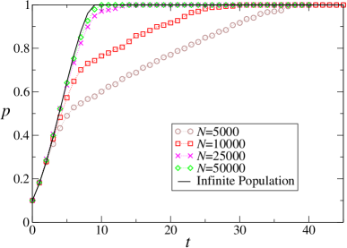
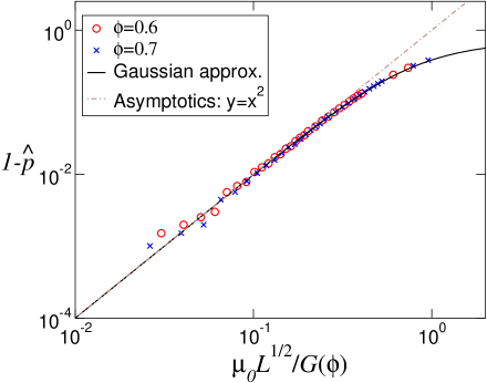
In the previous sections, we have assumed an infinite population, and comparison with simulations have shown that this approximation is appropriate most of the time. However, under the experimentally relevant situations, where very strong selection and very low mutation rate are employed, finite population effects can show up and be potentially important. As an extreme example, if we choose the best member from the population, i.e, $N\phi=1$, then recombination has nothing to work with and offers no benefit. In this section we discuss the population size above which the evolutionary dynamics and equilibrium can essentially be deemed the same as those of infinite populations. To rid ourselves of the impact of initial conditions, we assume an initially diversified population. Two population sizes are relevant for this problem, the total population size $N$ at the beginning of each generation, and the selected population size $N\phi$. We will focus on the case most often encountered in in vitro evolution experiments, namely $N$ very large, but $N\phi$ is rather small. In the following analysis, we set $\phi$ constant, and compare the evolutionary trajectory for different population sizes $N$. We start again from the simplest case of no point mutation, shown in Fig. (13a). It can be seen that in general the smaller the population size, the worse the evolutionary efficiency and the equilibrium state. Under these conditions, the finite population effect comes from the genetic association between loci that results in the loss of favorable alleles from the entire population when the population is subject to selection.

We can estimate the population size $N_{0}$ above which the population dynamic approaches infinite-population results by estimating the average number of lost favorable alleles at all loci in the selected population. As the individual match probability ${p}$ is lowest at the beginning of evolution, if there is any loss of favorable allele, it is most likely to happen at the first round of selection, hence we focus on the first round of selection and recombination. Right after the first round of selection, the probability for a specific locus to lose the favorable allele is $(1-{p}(1))^{N\phi}$. Therefore the average number of loci losing the favorable allele is $L(1-{p})^{N\phi}$. The opposite way of saying this is that for the population to retain favorable alleles at all loci after the first round of selection, we require $L(1-{p})^{N_{0}\phi}<1$. This gives the following estimate of $N_{0}$:

$$N_{0}=\frac{1}{\phi}\frac{-\ln L}{\ln(1-{p}(1))},$$ (33)

where ${p}(1)={p}(0)+G(\phi)\sqrt{{p}(0)(1-{p}(0))/L}$. If in the first round the above criterion is met, then it is more unlikely for the population to lose any favorable alleles any at successive rounds when subject to selection, as ${p}(t)$ increases in later rounds and $L(1-{p})^{N\phi}$ becomes increasingly smaller than $1$. Comparison with simulation results shows that Eq. (33) gives a reasonable estimate (at least correct in order of magnitude).

When a (weak) point mutation is involved, the dynamics can be separated into two regimes: (a) recombination dominated evolution, where for loci that have a favorable allele in them, recombination helps that favorable loci to spread to the whole population, as in the mutation-free case, and (b) mutation/recombination evolution, where loci that have lost their favorable alleles due to selection need mutations to find them again. The dynamics in this regime is significantly slower, as seen in Fig. (13b). In this case, Eq. (33) still identifies the smallest population size $N_{0}$ that behaves more or less like an infinite population. As a side note, the flip side of the finite population issue is that there exists an optimal selection pressure for a particular population size; an estimate of this optimal $\phi$ can be found from the condition $L(1-{p})^{N\phi}<1$.

The estimate of $N_{0}$ given $\phi$ (or equivalently the optimal $\phi_{0}$ given $N$) has practical implications. It gives a population size that is just enough for the evolution to proceed in its fastest rate (given a selection strength). Since in real-life experiments selection routinely involves screening the population, which is costly and time-consuming, a smaller while still equally effective population size would be helpful. Of course, the above arguments assumed a random initial library. If one starts from a population of a single clone, then as already explained above, even at the beginning mutation is absolutely necessary to generate diversity. For this case it is more difficult to directly estimate the finite population effects.

DISCUSSION

In this work we proposed and studied a simplified model of DNA shuffling, a very important evolutionary protocol for directed evolution. We investigated this model from a population genetics’ point of view, as a multi-locus evolutionary model incorporating both recombination and point mutation and subject to dynamical truncation selection. Our specific recombination scheme, as an extreme limit of multi-parent multi-crossover genetic mixing employed in DNA shuffling, enables us to pursue analytical results for the dynamical and equilibrium features. To summarize, we derived the recursion relations that completely characterize the evolutionary process, which shows explicitly how recombination helps to speed up the evolution. Assuming a large number of loci, we found that selection and mutation affect the evolutionary process only through a combination of their respective parameters. When the evolution is relatively slow so that the discrete recursion relation can be approximated by a continuous differential equation, we could solve for the evolutionary trajectory, and prove in special cases that it is indeed faster than that for the case of no-recombination. We also investigated the equilibrium properties of the system, and found that the genetic load when recombination is in effect has a different scaling form than usual, as long as the selection is not super strong. In addition, we discussed the finite-size effect under conditions relevant to the shuffling experiments, and estimated the minimal population size above which the population behaves as if an infinite population.

We have been focusing on a model which is directly relevant only under very specific conditions, but our results are actually applicable to broader situations. Let us first discuss selection:(a) For simplicity, we employed a dynamical truncation selection. In the case of DNA sequence evolution via binding to protein, selection is “smoother” [roughly speaking, the step corners are rounded (VON HIPPEL and BERG $1986$; GERLAND and HWA $2002$)]. This simplification does not cause any substantial difference in our analytical results as long as the binding affinity is large (i.e, the step is steep enough). (b) Our approach and results are also applicable to the type of dynamical (soft) selection studied by Kondrashov ($1995$). There, the selection is implemented as a function $W(X)$, where $X=({m}-\overline{{m}})/\sigma$, i.e., the phenotypic difference between the phenotype and the mean $\overline{m}$, divided by the standard deviation $\sigma$ of the phenotypic distribution. The effect of this type of selection on a population with a Gaussian distribution is

$${m}_{\rm s}-{m}=\sigma\delta,$$ (34)

where $\delta$ is a quantity solely characterized by the selection function $W(X)$ and does not depend on the population phenotypic distribution [See Eqs.($7$) and ($14$) of Kondrashov ($1995$)]. It is evident that Eq. (34) is analogous to Eq. (5) except that one needs to replace $G(\phi)$ with $\delta$. Therefore, when one exchange $G(\phi)$ with $\delta$, all our results under the Gaussian approximation remain valid, including various scaling arguments and solutions to the continuous evolutionary equations.

Now we move to recombination. One immediate question is what would change when the recombination scheme is more realistic. A straightforward generalization of the maximal recombination toward the realistic situation is that we can cut each DNA sequence into segments of equal length, with the maximum recombination as the extreme case of length equal to $1$. Computer simulation shows that in general the longer the segment length, the worse the performance. For a general segment length, one can derive a hierarchy of recursion relations that relate the cumulants of the population distribution at the current generation to those of previous generation, an approach that has been applied to a multi-locus system on a fixed landscapes (BARTON and TURELLI $1991$; BÜGER $2000$). How to close the chain of recursion relations remain to be studied. The difficulty is associated with the remaining linkage within each segment. In any event, the maximal recombination model can serve as a theoretical upper limit which is qualitatively correct and even reasonably accurate quantitatively.

Our study has been guided by the in vitro evolution process, where the intensity of recombination and mutation are both prescribed by the experimenter. This might be not be the case in a more natural setting, where the evolution of recombination (mutation) itself can be an important aspect of the problem (e.g., FELDMAN et.al. $1996$). Therefore our model does not incorporate a modifier gene that explicitly controls recombination rate. In such a modifier approach, the recombination rate can itself evolve because the modifier gene is under indirect selection due to its association with other genes on the same chromosome under direct selection (e.g., FELDMAN et.al. $1996$).

Finally, we believe that our model may be relevant to some examples of natural evolution: (a) dynamical truncation selection can also exist in nature, for example the mutual selection in a host-parasite system and (b) recombination of multi-parents, multi-crossover type does exist in nature: certain RNA viruses have multiple segments in their genome, and when multiple viruses infect the same host and new virus particles are made, recombination of the type we study can happen (CHAO $1988$). With the ease of analytical treatment of this model, we hope it can serve as a theoretical testing ground where general statements about the interplay among various aspects such as recombination, mutation and selection, can be tried out.

We would like to give special thanks to L. Chao for stimulating discussions. We also acknowledge helpful interactions with S. P. Otto, A. Poon, W. P. C. Stemmer and J. Widom. This work has been partially funded by the NSF sponsored Center for Theoretical Biological Physics (grants # PHY-0216576 and 0225630).

Appendix A Explicit solution of the evolution equation

Assuming that at $t=0$ the individual match probability is ${p}(0)$, the explicit solution for the continuous version of Eq. (18)(which is a good approximation when change of ${p}$ in between consecutive rounds is small, i.e., when selection is not very strong) is

$$\frac{d{p}}{dt^{\prime}}=(1-{\mathcal{A}}{p})+C\sqrt{{p}(1-{p})},$$ (35)

where $t^{\prime}\equiv({\mu_{0}}/({\mathcal{A}}-1))t$ and $C\equiv({\mathcal{A}}-1)G(\phi)/({\mu_{0}}\sqrt{L})$. For most parameter ranges the righthand side is positive, therefore ${p}$ keeps increasing.

The general solution of Eq. (35) is:

$$\frac{{\mathcal{A}}^{2}+C^{2}}{2}t^{\prime}=-\frac{{\mathcal{A}}}{2}\ln\frac{\left|1-{\mathcal{A}}{p}+C\sqrt{{p}(1-{p})}\right|}{\left|1-{\mathcal{A}}{p}(0)+C\sqrt{{p}(0)(1-{p}(0))}\right|}+\frac{C(1-{\mathcal{A}}/2)}{\sqrt{\Delta}}$$

$$\qquad\qquad\times\left[\ln\frac{\left|2\sqrt{(1-{p})/{p}}+{C}-\sqrt{\Delta}\right|}{2\sqrt{(1-{p})/{p}}+{C}+\sqrt{\Delta}}-\ln\frac{\left|2\sqrt{(1-{p}(0))/{p}(0)}+{C}-\sqrt{\Delta}\right|}{2\sqrt{(1-{p}(0))/{p}(0)}+{C}+\sqrt{\Delta}}\right]$$

$$\qquad\qquad-C\left(\tan^{-1}\sqrt{\frac{1-{p}}{{p}}}-\tan^{-1}\sqrt{\frac{1-{p}(0)}{{p}(0)}}\right),$$ (36)

where $\Delta\equiv C^{2}-4(1-{\mathcal{A}})$. In the absence of mutation the above equation has been solved, the solution a sinusoidal function (see Eq. (12). The other extreme situation is when selection strength $\phi$ is $1$, which leads to $G(\phi)=0$ and $C=0$. In this case ${p}$ goes to $1/{\mathcal{A}}$ exponentially with time constant $-\ln(1-{\mathcal{A}}{\mu_{0}}/({\mathcal{A}}-1))\approx{\mathcal{A}}{\mu_{0}}/({\mathcal{A}}-1)$.

Appendix B Arbitrary chromosome length $L$

In the discussion of the evolutionary dynamics and equilibrium state, we make use of a Gaussian (and a Poisson distribution ) to approximate a binomial distribution, which are valid when $L\gg 1$. In fact, one can relax this condition and work directly with binomial distribution, with the help of special function $I_{x}(a,b)$, the incomplete Beta function. $I_{x}(a,b)$ is defined as

$$I_{x}(a,b)=\frac{1}{B(a,b)}\int_{0}^{x}dtt^{a-1}(1-t)^{b-1},$$ (37)

where $B(a,b)$ is the complete beta function.

Suppose the probability density for a binomial distribution is

$$P_{{p}}({m},L)\equiv C_{L}^{{m}}{p}^{{m}}(1-{p})^{L-{m}}.$$ (38)

The cumulative probability density is then

$$\sum_{i={m}}^{L}P_{{p}}(i,L)=I_{{p}}({m},L+1-{m})$$ (39)

We have, at the selection,

$$\phi=\alpha P_{{p}}({{m}_{0}},L)+\sum_{i={{m}_{0}}+1}^{L}P_{{p}}(i,L),$$ (40)

where again ${{m}_{0}}$ is the threshold and the state with ${{m}_{0}}$ matches maybe partially selected.

The new individual match probability after selection and recombination is

$$L{p}^{\textrm{r}}=\frac{1}{\phi}\left(\alpha{{m}_{0}}P_{{p}}({{m}_{0}},L)+\sum_{i={{m}_{0}}+1}^{L}iP_{{m}}(i,L)\right)$$ (41)

Incorporating the mutational process and making use of Eq. (40), we arrive at

$${p}_{t+1}=\frac{{\mu_{0}}}{{\mathcal{A}}-1}+\frac{1-\frac{{\mathcal{A}}}{{\mathcal{A}}-1}{\mu_{0}}}{L\phi}\left({{m}_{0}}\phi+L{p}_{t}I_{{p}_{t}}({{m}_{0}},L-{{m}_{0}})-{{m}_{0}}I_{{p}_{t}}(k{{m}_{0}}+1,L-{{m}_{0}})\right),$$ (42)

where we made use of the following identity

$$\sum_{i={{m}_{0}}+1}^{L}iP_{{p}}(i,L)=L{p}I_{{p}}({{m}_{0}},L-{{m}_{0}}).$$ (43)

The dynamics and equilibrium properties follow from Eq. (42). Fig. (14) shows that, when chromosome length $L$ is not long, indeed this approach agrees much better with simulation than Gaussian approximation.

Figure 14: Comparison of two theoretical approaches with simulation result. Solid curve is the result of Eq. (42). Dashed curve is the result of Eq. (17). Here $L=10$, $\phi=.9$ and ${\mu_{0}}=.001$. In simulation $N=10^{4}$.

References

- ARNOLD, [2001] ARNOLD, F. H., 2001. Combinatorial and computational challenges for biocatalyst design. Nature, 409, 253–257.
- BARLOW and HALL, [2002] BARLOW, M., and B. G. HALL 2002. Predicting evolutionary potential: In vitro evolution accurately reproduces natural evolution of the TEM betalactamase. Genetics, 160, 823–832.
- BARTON and TURELLI, [1991] BARTON, N. H., and M. TURELLI, 1991. Natural and sexual selection on many loci. Genetics, 127, 229–255.
- BEYER, [2001] BEYER, HANS-GEORG, 2001. The Theory of Evolution Strategies. Berlin: Springer-Verlag Harper.
- BÜGER, [2000] BÜGER, R., 2000. The Mathematical Theory of Selection, Recombination and Mutation. Chichester: Jon Wiley and Sons LTD.
- CHAO, [1988] CHAO, L., 1988. Evolution of Sex in RNA Viruses. J. theor. Biol., 133, 99–112.
- COHEN and KESSLER, [2003] COHEN, E., and D. A. KESSLER, 2003. Equilibrium state of molecular breeding. cond-mat/0301503.
- CROW and KIMURA, [1970] CROW, J. F., and M. KIMURA, 1970. An introduction to population genetics theory. New York: Harper and Row Publishers Inc.
- FARINAS et al. , [2001] FARINAS, E. T., T. BULTER, and F. H. ARNOLD, 2001. Directed enzyme evolution. Curr. Opin. Biotechnol., 12, 545–551.
- FELDMAN et al. , [1996] FELDMAN, M. W., S. P. OTTO, and F. B. CHRISTIANSEN, 1996. Population genetic perspectives on the evolution of recombination. Annual Review of Genetics, 30, 261–295.
- GERLAND and HWA, [2002] GERLAND, U., and T. HWA, 2002. On the selection and evolution of regulatory DNA motifs. J. Mol. Evol., 55, 386–400.
- KESSLER et al. , [1997] KESSLER, D. A., H. LEVINE, D. RIDGWAY, and L. TSIMRING, 1997. Evolution on a smooth landscape. J. Stat. Phys., 87, 519–544.
- KIMURA and CROW, [1978] KIMURA, M., and J. F. CROW, 1978. Effect of overall phenotypic selection on genetic change at individual loci .1. Proc. Natl. Acad. Sci. U. S. A., 75, 6168–6171.
- KONDRASHOV, [1995] KONDRASHOV, A. S., 1995. Dynamics of unconditionally deleterious mutations - gaussian approximation and soft selection. Genet. Res., 65, 113–121.
- KURTZMAN et al. , [2001] KURTZMAN, A. L., S. GOVINDARAJAN, K. VAHLE, J. T. JONES, V. HEINRICHS, and P. A. PATTEN, 2001. Advances in directed protein evolution by recursive genetic recombination: applications to therapeutic proteins. Curr. Opin. Biotechnol., 12, 361–370.
- LODISH et al. , [1999] LODISH, H., A. BERK, S. L. ZIPURSKY, P. MATSUDAIRA, D. BALTIMORE, and J. DARNELL, 1999. Molecular Cell Biology, th Ed. New York: W. H. Freeman and Co.
- MOORE and MARANAS, [2000] MOORE, G. L., and C. D. MARANAS, 2000. Modeling DNA Mutation and Recombination for Directed Evolution Experiments. J. Theor. Biol., 205, 483–503.
- MÜHLENBEIN and SCHLIERKAMP-VOOSEN, [1993] MÜHLENBEIN, H., and D. SCHLIERKAMP-VOOSEN, 1993. The Science of Breeding and Its Application to the Breeder Genetic Algorithm (BGA). Evolutionary Computation, 1, 335–360.
- ORENCIA et al. , [2001] ORENCIA, M. C., J. S. YOON, J. E. NESS, W. P. C. STEMMER, and R. C. STEVENS, 2001. Predicting the emergence of antibiotic resistance by directed evolution and structural analysis. Nat. Struct. Biol., 8, 238–242.
- OTTO and BARTON, [2001] OTTO, S. P., and N. H. BARTON, 2001. Selection for recombination in small populations. Evolution, 55, 1921–1931.
- OTTO and LENORMAND, [2002] OTTO, S. P., and T. LENORMAND, 2002. Resolving the paradox of sex and recombination. Nat. Rev. Genet., 3, 252–261.
- PENG et al. , [2003] PENG, W., U. GERLAND, T. HWA, and H. LEVINE, 2003. Dynamics of Competitive Evolution on a Smooth Landscape. To appear in Phys. Rev. Lett.
- SHNOL and KONDRASHOV, [1993] SHNOL, E. E., and A. S. KONDRASHOV, 1993. The effect of selection on the phenotypic variance. Genetics, 134, 995–996.
- STEMMER, [1994a] STEMMER, W. P. C., 1994a. Dna shuffling by random fragmentation and reassembly - in-vitro recombination for molecular evolution. Proc. Natl. Acad. Sci. U. S. A., 91, 10747–10751.
- STEMMER, [1994b] STEMMER, W. P. C., 1994b. Rapid evolution of a protein in-vitro by DNA shuffling. Nature, 370, 389–391.
- SUN, [1999] SUN, F., 1999. Modeling DNA shuffling. J. Comp. Biol., 6, 77–90.
- THASTROM et al. , [1999] THASTROM, A., P. T. LOWARY, H. R. WIDLUND, H. CAO, M. KUBISTA, and J. WIDOM, 1999. Sequence motifs and free energies of selected natural and nonnatural nucleosome positioning DNA sequences. J. Mol. Biol., 288, 213–229.
- VON HIPPEL and BERG, [1986] VON HIPPEL, P. H., and O. G. BERG, 1986. On the specificity of DNA-protein interactions. Proc. Natl. Acad. Sci. U. S. A., 83, 1608–1612.