Control of cardiac alternans in a mapping model with memory
Abstract
We investigate a map-based model of paced cardiac muscle in the presence of closed-loop feedback control. The model relates the duration of an action potential to the preceding diastolic interval as well as the preceding action potential duration and thus has some amount of ‘memory.’ We find that the domain of control depends on this memory, independently of the specific functional form of the map. The memory-dependent domain of control can encompass large feedback gains, thus providing the first possible explanation of the recent experimental results of Hall et al. [Phys. Rev. Lett, 88, 198102 (2002)] on controlling alternans in small pieces of rapidly-paced cardiac muscle.
pacs:
05.45.-a, 87.19.Hh, 87.10.+eSudden cardiac death, primarily caused by ventricular arrhythmias, is a major public health problem: it is one of the leading causes of mortality in the western world. A possible precursor of some arrhythmias is the beat-to-beat variation of the cardiac electrical excitation occurring at fast heart rates karma ; gilmour1 . This variation appears as a sequence of long-short-long-short cycles (termed alternans) in important physiological characteristics such as action potential duration (APD) and conduction time. A focus of recent theoretical and experimental studies is to investigate the mechanisms causing alternans and to terminate this response pattern using closed-loop feedback methods developed by the nonlinear dynamics community. Suppressing such alternans may then prevent the onset of fibrillation karma1 .
Over the last few years, several studies have demonstrated that alternans can be suppressed with dynamic feedback control of the pacing interval dan ; hall ; karma2 ; dan1 ; christini . Control of alternans in the conduction time across the atrioventricular (AV) node has been demonstrated in both in vitro rabbit hearts hall and in vivo human hearts christini . The observed AV-nodal alternans are known to be well described by a one-dimensional map-based mathematical model christini . The model can be used to predict the range of control parameters that stabilize the desired response patterns.
Recently, Hall et al. dan demonstrated successful control of alternans in small pieces of in vitro paced bullfrog ventricles. Understanding how to control ventricular myocardium is important because it is the primary substrate for fibrillation. Controlling alternans in ventricular myocardium was expected to be more difficult than controlling AV-nodal alternans because past research suggests that its dynamics is more complicated. On the contrary, the experiments described in Ref. dan demonstrated that alternans could be suppressed over a wide range of control parameters and over the entire range of pacing rates for which alternans was observed. The observations were compared to the predictions of two map-based mathematical models. Fitting the bifurcation diagrams of the mathematical models to the experimental data did not produce good fits for their domains of control. Specifically, control of alternans was observed for feedback gains as large as four in the experiments, whereas the models predicted that the gain must be less than and limited to a small region of pacing rates near the bifurcation to alternans.
The primary purpose of this Letter is to analyze a map-based model of paced cardiac muscle in the presence of closed-loop feedback control. The model contains some degree of ‘memory’ so its dynamics displays higher-dimensional behavior. We find that the domain of control can encompass large feedback gains, qualitatively consistent with the experiments of Hall et al. Our results demonstrate that higher-dimensional effects can enhance the effectiveness of control under the appropriate conditions. This may lead eventually to the development of methods for in vivo control of whole-heart functions. Future experiments are needed to determine whether the specific form of memory considered here is displayed by cardiac tissue. Nevertheless, our results indicate the importance of memory in the control of alternans.
To set the stage for understanding the behavior of the higher-dimensional model, we first consider a simpler one-dimensional map that contains no memory. This mapping model is given by nolasco ; guevara
| (1) |
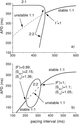
where is the APD generated by the stimulus, and is the diastolic interval (DI), i.e. the interval during which the tissue recovers to its resting state after the end of the previous () action potential. We illustrate a typical bifurcation diagram in Fig. 1a. Note that the tissue has a stable 1:1 response pattern (every stimulus elicits an action potential of equal duration) for long pacing intervals (slow pacing rate). As the pacing interval decreases (faster pacing), the 1:1 response becomes unstable and a transition to alternans (2:2 response) occurs. At even faster pacing rates, the 2:2 response pattern becomes unstable and is replaced by a stable 2:1 response where an action potential is produced by every second stimulus. For the 1:1 and 2:2 responses considered herein, the pacing relation between APD and DI is , where is the basic pacing interval.
For this simple model, the transition from 1:1 to 2:2 behavior shown in the Fig. 1a can be understood by investigating the restitution properties of the cardiac membrane. Specifically, to predict the pacing rates at which the 1:1 response is stable, one constructs the restitution curve (RC) by plotting APD as a function of the preceding DI, as in (1). Nolasco and Dahlen nolasco proposed that the transition to alternans occurs when the slope of the RC is equal to unity. However, recent studies dan ; dan2 ; fox ; gray ; lena1 have shown that the slope of the RC at the onset of alternans can be significantly larger than unity and thus this criterion fails to predict the existence of alternans in some cases. Later in the paper, we analyze the map (1), independently of the specific form of the function , in the presence of closed-loop feedback control and discuss why it fails to explain the experimental observations.
In contrast to the memoryless model (1), we find that a cardiac mapping model of the form
| (2) |
can possess a domain of control that encompasses large control gains, independently of the specific form of . This model has some amount of memory because it relates the duration of the next action potential both to the previous DI and to the previous APD, i.e., the history of the dynamical system. Several previous studies dan2 ; otani ; chialvo ; gilmour2 indicate that higher-dimensional behavior (so-called memory effects) is present in real cardiac tissue and thus has to be taken into account in order to correctly predict the onset of alternans. The general form of this model was first introduced by Otani and Gilmour otani to explain empirical observations from paced dog cardiac Purkinje fibers. More recently, a specific form of was derived analytically lena from a three-current ionic model FK .
Our analysis of the model (2) shows that it displays rate-dependent restitution so that there exist two primary types of RCs (the dynamic and S1-S2 RCs), which can be measured independently using different pacing protocols lena1 . In the dynamic pacing protocol, the pacing interval is held fixed until the tissue reaches equilibrium, and then progressively shortened. This yields pairs of steady-state values () for each . In the S1-S2 pacing protocol, a premature stimulus (“S2”) is delivered at an interval after pacing the tissue with a sufficiently large number of “S1” stimuli at a pacing interval so that the tissue reaches equilibrium. The S1-S2 RC is determined by measuring the resulting APD for various coupling intervals . Experimental studies have shown that the S1-S2 and dynamic RCs differ significantly, and have different slopes (denoted as and respectively). This is consistent with the predictions of the mapping model (2). The transition to alternans is governed by the combination of the slopes and , so that alternans can exist when
| (3) |
where is the full derivative of , with respect to , evaluated at a fixed point lena1 . Note that when there is no memory in the model, and that they differ substantially when there is large memory. A typical bifurcation diagram showing alternans in the mapping model (2) is presented in Fig. 1b, where the slopes of the RCs are different and do not equal unity at the onset of alternans.
We now consider control of alternans in both models (1) and (2). To suppress alternans and stabilize the 1:1 pattern, Hall et al. dan adjusted the pacing period by an amount given by
| (4) |
where is the feedback gain. Control is initiated by adjusting the basic pacing interval by . Applying the control technique to the mapping model (1) yields
| (5) |
The linearization of (5) in a neighborhood of the fixed point (when and ) is
| (6) |
where denotes evaluation at the fixed point. Since the controlled pacing relation is , the derivatives in (6) are
| (7) |
We rewrite expressions (4) and (6) in matrix form as
| (8) |
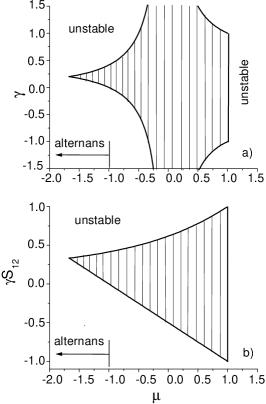
where , , and . Control is successful when the eigenvalues of (8) fall within the unit circle in the complex plane. This occurs when and lie within the region defined by the curves
| (9) |
as shown in Fig. 2a. Condition (9) defines the domain of control for the mapping model (1). Note that the domain does not depend on the specific functional form of , but only on the value of its derivative evaluated at the fixed point. Alternans may exist in the uncontrolled mapping model (1) when The domain of control indicates the values of the gain that should be used to establish control of alternans for different values of the Floquet multiplier , which describes the stability of the map in the absence of control. Note that the gain necessary to establish control in the region where alternans exist in the absence of control is small ( in contradiction with the experimental observations dan where can be as large as 4.
Very different behavior is found for the mapping model (2) with memory. In the presence of control, Eq. (2) becomes
| (10) |
Linearizing (10) in a neighborhood of the fixed point, we find that
| (11) |
where
| (12) |
As in Eq. (7), we denote as a full derivative of , evaluated at the fixed point. As seen from Eq. (3), the condition for the existence of alternans in the absence of control is given by Note that the value of does not predict the existence of alternans; instead, it characterizes the immediate response of the tissue to small perturbations from the fixed point, as was shown in Ref. lena1 . Hence, we expect that is more relevant for determining the effects of control, whereas dictates the stability of the steady-state response of the tissue.
| (13) |
The only difference between the matrices describing the controlled dynamics for the maps with and without memory is the term containing the control gain . In the memoryless mapping model (1), the magnitude of perturbation sensitivity is proportional to the full derivative , whereas it is proportional to the slope of the S1-S2 RC in the mapping model with memory (2). When there is no memory, , whereas they can differ substantially when memory is present.
By analyzing (13), we find that control is successful when and lie within the region defined by the curves
| (14) |
Similar to the previous model, the domain of control (14) does not depend on the specific form of the function . We only need to know the values of the full derivative and the slope of the S1-S2 RC (evaluated at the fixed point) to determine whether it is possible to establish control. Figure 2b depicts the domain of control for the one-dimensional mapping model with memory (2) according to conditions (14). Alternans may exist in the uncontrolled system when It can be seen from Fig. 2b that the value of necessary to establish control for this region is relatively small (). However, the actual control gain can be larger or smaller than this range depending on the value of . Our predictions are consistent with our earlier expectations that influences the effects of control since it quantifies the response of the tissue (in equilibrium) to a sudden perturbation, which the controller attempts to cancel.
Comparing our predictions to experiments is not possible at this time because no experiments have measured the slope of the S1-S2 RC evaluated at the fixed point note . Most of the experiments (see, for instance, Refs. gilmour2 ; mary ) used S1-S2 pacing protocol in which the “S1” interval was either fixed or set to only a few different values. Instead, to make a direct comparison of the domain of control obtained using mapping model (2) to the one obtained experimentally in Ref. dan , we need to know the slope of the S1-S2 RC at each point on the dynamic RC, i.e., for different S1. The value can be greater or less than one, depending on the specific form of or the specific type of tissue. For example, for the function used to generate the plot shown in Fig. 1b. Hence, the control gain must be less than ( to be in the region where control is effective. However, preliminary, experiments with bullfrog cardiac muscle indicate that can be relatively small (less than 0.4 and as small as 0.05) at the onset of alternans soma and thus the control gain could be large.
Thus, the experimentally measured domain of control may be consistent with the predictions of the controlled map with memory (2) if is truly less than one in bullfrog. The map without memory (1) does not agree with experiments as demonstrated by Fig. 2a and as noted previously in Ref. dan . Our analysis is the first to suggest that memory effects may substantially enlarge the domain of control, regulated by Future experiments are needed to clarify the effects of memory on control.
A limitation of our analysis is that the extent of cardiac memory is only one previous beat in the model (2), so that the memory is short-term. However, some studies indicate that long-term memory effects are present in real cardiac tissue mary that might be described using a long-term memory mapping model fox ; chialvo . In this model, an additional memory variable is introduced, which is assumed to accumulate during the APD and dissipate during the DI. Analysis of this model fox confirms that the slope of the dynamic RC does not predict the transition to alternans, but it was shown in Ref. dan that a specific form of such a memory model cannot explain the experiments on control of alternans. We believe that a generalization of the mapping model (2) that includes long-term memory as in fox ; chialvo may be a fruitful direction for future investigations.
We gratefully acknowledge the support of the National Science Foundation under Grant PHY-9982860 and DMS-9983320 (M.M.R).
References
- (1) A. Karma, Chaos 4, 461 (1994).
- (2) R.F. Gilmour, Jr., D.R. Chialvo, J. Cardiovasc. Electrophysiol. 10, 1087 (1999).
- (3) B. Echebarria, and A. Karma, Chaos 12, 533 (2002).
- (4) G.M. Hall, and D.J. Gauthier, Phys. Rev. Lett. 88, 198102 (2002).
- (5) K. Hall, D.J. Christini, M. Tremblay, J.J. Collins, L. Glass, and J. Billette, Phys. Rev. Lett. 78, 4518 (1997).
- (6) W.-J. Rappel, F. Fenton and A. Karma, Phys. Rev. Lett. 83, 456 (1999).
- (7) D.J. Gauthier, and J.E.S. Socolar, Phys. Rev. Lett. 79, 4938 (1997).
- (8) D.J. Christini, K.M. Stein, S.M. Markowitz, S. Mittal, D.J. Slotwiner, M.A.Scheiner, S. Iwai, and B.B. Lerman, Proc. Nat. Acad. Sci. 98, 5827 (2001).
- (9) J.B. Nolasco, and R.W. Dahlen, J. Appl. Physiol. 25, 191 (1968).
- (10) M. Guevara, G. Ward, A. Shrier, and L. Glass, Computers in Cardiology (IEEE Computer Society, Silver Spring, MD, 1984), p.167.
- (11) G.M. Hall, S. Bahar, and D.J. Gauthier, Phys. Rev. Lett. 82, 2995 (1999).
- (12) J.J. Fox, E. Bodenschatz, and R.F. Gilmour, Phys. Rev. Lett. 89, 138101 (2002).
- (13) I. Banville, and R.A. Gray, J Cardiovasc. Electrophysiol. 13, 1141 (2002).
- (14) E.G. Tolkacheva, D.G. Schaeffer, D.J. Gauthier, and W. Krassowska, Phys. Rev. E. 67, 031904 (2003).
- (15) N.F. Otani, and R.F. Gilmour, Jr., J. Theor. Biol. 187, 409 (1997).
- (16) D.R. Chialvo, D.C. Michaels, and J. Jalife, Circ. Res. 66, 525 (1990).
- (17) R.F. Gilmour, Jr., N.F. Otani, and M.A. Watanabe, Am. J. Physiol. 272, H1826 (1997).
- (18) E.G. Tolkacheva, D.G. Schaeffer, D.J. Gauthier, and C.C. Mitchell, Chaos 12, 1034 (2002).
- (19) F. Fenton, and A. Karma, Chaos 8, 20 (1998).
- (20) We note that a pacing protocol has been suggested in [18] for easily determining , , and (evaluated at the fixed points) in experiments.
- (21) M.A. Watanabe, and M.L. Koller, Am. J. Physiol. 282, H1534 (2002).
- (22) S. Sau and H. Dobrovolny, private communication.