Permanent Address:] Department of Physics and Astronomy, Arizona State University, Tempe, AZ 85287, U.S.A.

Superfluid Fermi Gases with Large Scattering Length

Abstract

We report quantum Monte Carlo calculations of superfluid Fermi gases with short-range two-body attractive interactions with infinite scattering length. The energy of such gases is estimated to be $(0.44\pm 0.01)$ times that of the noninteracting gas, and their pairing gap is approximately twice the energy per particle. PACS: 03.75.Fi, 05.30.Fk, 21.65.+F

In dilute Fermi gases the pair interactions have a range much smaller than the interparticle spacing. However, when the two-particle scattering length is large, these short range interactions can modify the gas properties significantly. A well known example is low density neutron matter which may occur in the inner crust of neutron stars Pethick and Ravenhall (1995). The two-neutron interaction has a range of $\sim 2$ fm, but the scattering length is large, $-18$ fm, so that even at densities as small as one percent of the nuclear density the parameter $ak_{F}$ has magnitude much larger than one. Bertsch proposed in 1998 that solution of the idealized problem of a dilute Fermi gas in the limit $ak_{F}\rightarrow-\infty$ could give useful insights into the properties of low density neutron gas.

Cold dilute gases of ⁶Li atoms have been produced in atom traps. The interaction between these atoms can be tuned using a known Feshbach resonance; and the estimated value of $ak_{F}$ in the recent experiment O’Hara et al. (2002) is $\sim-7.4$. As the interaction strength is increased beyond that for $a=-\infty$, we get bosonic two-fermion bound states. In this sense a dilute Fermi gas with large $a$ is in between weak coupling BCS superfluid and dilute Bose gases with Bose-Einstein condensation Randeria (1995). Attempts to produce Bose gases in the limit, $a/r_{0}\rightarrow\infty$ using Feshbach resonances Stenger et al. (1999); Roberts et al. (2001), are in progress, and their energy has been recently estimated using variational methods Cowell et al. (2002).

In the $a\rightarrow-\infty$ limit $k_{F}^{2}/m$ is the only energy scale, and the ground state energy of the interacting dilute Fermi gas is proportional to the noninteracting Fermi gas energy:

$$E_{0}(\rho)=\xi~{}E_{FG}=\xi~{}\frac{3}{10}~{}\frac{k_{F}^{2}}{m}~{}.$$ (1)

Baker Baker (1999) and Heiselberg Heiselberg (2001) have attempted to obtain the value of the constant $\xi$ from expansions of the Fermi gas energy in powers of $ak_{F}$. Heiselberg obtained $\xi=0.326$, while Baker’s values are $\xi=0.326$ and $0.568$.

Fermi gases with attractive pair interaction become superfluid at low temperature. The BCS expressions in terms of the scattering length were given by Leggett Leggett (1980), and they were used to study the properties of superfluid dilute Fermi gases, as a function of $ak_{F}$, by Engelbrecht, Randeria and Sá de Melo Engelbrecht et al. (1997). For $ak_{F}=-\infty$ they obtain an upperbound, $\xi=0.59$, using the BCS wave function. These gases are also estimated to have large gaps comparable to the ground state energy per particle.

Here we report studies of Fermi gases with quantum Monte Carlo methods using the model potential:

$$v(r)=-\frac{2}{m}\frac{\mu^{2}}{\cosh^{2}(\mu r)}~{}.$$ (2)

The zero energy solution of the two-body Schrödinger equation with this potential is $\tanh(\mu r)/r$ and corresponds to $a=-\infty$. The effective range is $2/\mu$, and in order to ensure that the gas is dilute we use $\mu r_{0}>10$, where $r_{0}$ is the unit radius; $\rho r_{0}^{3}=3/4\pi$. All the results presented here are for $\mu r_{0}=12$; however some of the calculations were repeated for $\mu r_{0}=24$ and the results extrapolated to $1/\mu\rightarrow 0$.

We have carried out fixed node Green’s function Monte Carlo Anderson (1975) (FN-GFMC) calculations with trial wave functions of the form:

$$\Psi_{V}({\bf R})=\prod_{i,j^{\prime}}f(r_{ij^{\prime}})\Phi({\bf R})~{},$$ (3)

where $i,j,...$ and $i^{\prime},j^{\prime},...$ label spin up and down particles, and the configuration vector ${\bf R}$ gives the positions of all the particles. Only the antiparallel spin pairs are correlated in this $\Psi_{V}$ with the Jastrow function $f(r_{ij^{\prime}})$. The parallel spin pairs do not feel the short range interaction due to Pauli exclusion.

In FN-GFMC the $\Psi_{V}$ is evolved in imaginary time with the operator $e^{-H\tau}$ while keeping its nodes fixed to avoid the fermion sign problem. In the limit $\tau\rightarrow\infty$ it yields the lowest energy state with the nodes of $\Psi_{V}$. These nodes, and hence the FN-GFMC energies, do not depend upon the positive definite Jastrow function. Nevertheless it is useful to reduce the variance of the FN-GFMC calculation. In the present work we use approximate solutions of the two-body Schrödinger equation:

$$\left[-\frac{1}{m}\nabla^{2}+v(r)\right]f(r<d)=\lambda f(r<d)~{},$$ (4)

with the boundary conditions $f(r>d)=1$ and $f^{\prime}(r=d)=0$ Cowell et al. (2002). The value of $d$ is obtained by minimizing the energy calculated using variational Monte Carlo. Note that a dilute Fermi gas is stable even when $a\rightarrow-\infty$, unlike dilute Bose gases in the $a\rightarrow\infty$ limit.

The calculations are carried out in a periodic cubic box having $\rho L^{3}=N$. The single particle states in this box are plane waves with momenta ${\bf k}_{i}$:

$${\bf k}_{i}=\frac{2\pi}{L}(n_{ix}{\hat{x}}+n_{iy}{\hat{y}}+n_{iz}{\hat{z}})~{}.$$ (5)

The free-particle energies depend only on $I=n_{x}^{2}+n_{y}^{2}+n_{z}^{2}$. For $N=14$ and 38 we have closed shells having states with $I\leq 1$ and $I\leq 2$ occupied. The commonly used Jastrow-Slater (JS) $\Psi_{V}({\bf R})$ is obtained by using:

$$\Phi_{\rm S}=[{{\cal A}}\prod_{I<I_{\rm max}}e^{i{\bf k_{i}}\cdot{\bf r}_{j}}][{{\cal A}}\prod_{I<I_{\rm max}}e^{i{\bf k_{i}}\cdot{\bf r}_{j}^{\prime}}]~{},$$ (6)

in Eq. 3. The more general, Jastrow-BCS $\Psi_{V}({\bf R})$ has:

$$\Phi_{\rm BCS}={{\cal A}}[\phi(r_{11^{\prime}})\phi(r_{22^{\prime}})...\phi(r_{nn^{\prime}})]~{},$$ (7)

with $n=N/2$. The antisymmetrizer ${{\cal A}}$ in the $\Phi_{\rm BCS}$ separately antisymmetrizes between the spin up and down particles. The $\Phi_{\rm BCS}$ describes the component of the BCS state with $N$ particles when

$$|{\rm BCS}\rangle = \prod_{i}(u_{i}+v_{i}a^{\dagger}_{{\bf k}_{i}\uparrow}a^{\dagger}_{{-\bf k}_{i}\downarrow})|0\rangle~{},$$ (8)

$$\phi(r) = \sum_{i}\frac{v_{i}}{u_{i}}e^{i{\bf k}_{i}\cdot{\bf r}}~{}.$$ (9)

The nodal surfaces of $\Phi_{BCS}$ depend upon the pairing function $\phi(r)$, and equal those of $\Phi_{S}$ when $v_{i}=0$ for all $k_{i}>k_{F}$.

FN-GFMC gives upperbounds to the energy, which equal the exact value when the trial wave function has the nodal structure of the ground state. Therefore, we can determine the $\phi(r)$ variationally by minimizing the FN-GFMC energy. We use the parameterization:

$$\phi({\bf r}) = \tilde{\beta}(r)+\sum_{i,~{}I\leq I_{C}}\alpha_{I}\exp[i\bf{k}_{i}\cdot{\bf r}]~{},$$ (10)

$$\tilde{\beta}(r) = \beta(r)+\beta(L-r)-2\beta(L/2)~{},$$ (11)

$$\beta(r) = [1+\gamma br]\ [1-\exp[-cbr]]\frac{\exp[-br]}{cbr}~{}.$$ (12)

The function $\tilde{\beta}(r)$ has a range of $L/2$, the value of $\gamma$ is chosen such that it has zero slope at the origin, and $I_{C}=4$ here.

Figure 1: The optimum $\phi({\bf r})$ (solid lines) and the $\phi_{S}$ (dashed lines) for $N=38$. Curves ending at $L/2$, $L/\sqrt{2}$ and $L\sqrt{3/4}$ are in the 001, 011 and 111 directions of the periodic box.

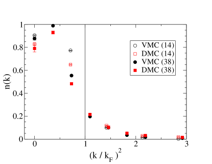
Figure 2: The momentum distribution of particles

The parameters $b,c$ and $\alpha_{I\leq I_{C}}$ of $\phi({\bf r})$ are optimized by choosing a random distribution of initial values and measuring the parameters of the lowest-energy (longest-lasting) configurations in FN-GFMC calculation. For 38 particles it produces an optimum set of parameters $br_{0}=0.8$, $c=10$, $\alpha_{I=0,4}=0.016,0.466,0.0068,0.00091,0.0007$ which give the smallest FN-GFMC energy having $\xi=0.440(2)$. Calculations in which $\beta(r)=0$ give optimum values $\alpha_{I=0,4}=0.24,1.0,0.2,0.057,0.035$ and $\xi=0.459(2)$, while the Slater $\phi_{S}({\bf r})$ having $\beta(r)=0$ and $\alpha_{I=0,4}=1,1,1,0,0$ gives a much larger $\xi=0.54$.

The optimum $\phi({\bf r})$ is compared with the $\phi_{S}({\bf r})$ in Fig. 1; it has a sharper peak at $r=0$. This peak depends upon the Jastrow function $f(r)$ acting between all the $N^{2}/4$ antiparallel spin pairs. For example, the $\phi(r)$ obtained by solving the BCS equation with the bare potential in uniform gas without the $f(r)$ has a much sharper peak.

The optimum $\phi({\bf r})$ has $\alpha_{0}<\alpha_{1}$ for N = 38; in contrast the variationally determined BCS wave function has $\alpha_{0}\geq\alpha_{1}$. The momentum distribution of particles in the trial and evolved ($\tau=0$ and $\infty$) wave functions are shown in Figure 2. For N = 38 the occupation of the $I=0$ state is smaller than the $I=1$, calculations with much larger values of $N$ are planned to test if this is a finite box size effect.

We have attempted further optimizations by incorporating backflow Feynman and Cohen (1956); Schmidt et al. (1981) into the BCS pair functions $\tilde{\phi}$. Initial calculations indicate that this will reduce the $\xi$ by $\approx$ 0.02. On the other hand, estimates of the corrections due to the finite range of the present interaction indicate that going to the $1/\mu\rightarrow 0$ limit will raise $\xi$ by a similar amount. Thus our present upperbound for the constant $\xi$ is 0.44(1).

In order to estimate the gap $\Delta$ of this superfluid we studied differences between energies of systems with odd and even number of particles. A general wave function with $n$ pairs, $u$ spin up and $d$ spin down unpaired particles can be written as:

$$\Phi_{\rm BCS}(R)={{\cal A}}\left\{\left[\phi(r_{11^{\prime}})...\phi(r_{nn^{\prime}})\right]\left[\psi_{1\uparrow}({\bf r}_{n+1})...\psi_{u\uparrow}({\bf r}_{n+u})\right]\left[\psi_{1\downarrow}({\bf r}_{(n+1)^{\prime}})...\psi_{d\downarrow}({\bf r}_{(n+d)^{\prime}})\right]\right\}~{}.$$ (13)

The unpaired particles are in $\psi_{i\uparrow}$ and $\psi_{j\downarrow}$ single particle states. We can write this wave function as the determinant of an $M\times M$ matrix where $M=n+u+d$ Bouchaud et al. (1988). For example, when $u=2$ and $d=3$ the matrix is given by:

$$\left(\begin{array}[]{cccccc}\phi(r_{11^{\prime}})&\phi(r_{12^{\prime}})&...&\phi(r_{1(n+d)^{\prime}})&\psi_{1\uparrow}({\bf r}_{1})&\psi_{2\uparrow}({\bf r}_{1})\\ \phi(r_{21^{\prime}})&\phi(r_{22^{\prime}})&...&\phi(r_{2(n+d)^{\prime}})&\psi_{1\uparrow}({\bf r}_{2})&\psi_{2\uparrow}({\bf r}_{2})\\ \vdots&\vdots&\vdots\vdots\vdots&\vdots&\vdots&\vdots\\ \phi(r_{(n+u)1^{\prime}})&\phi(r_{(n+u)2^{\prime}})&...&\phi(r_{(n+u)(n+d)^{\prime}})&\psi_{1\uparrow}({\bf r}_{n+u})&\psi_{2\uparrow}({\bf r}_{n+u})\\ \psi_{1\downarrow}({\bf r}_{1^{\prime}})&\psi_{1\downarrow}({\bf r}_{2^{\prime}})&...&\psi_{1\downarrow}({\bf r}_{(n+d)^{\prime}})&0&0\\ \psi_{2\downarrow}({\bf r}_{1^{\prime}})&\psi_{2\downarrow}({\bf r}_{2^{\prime}})&...&\psi_{2\downarrow}({\bf r}_{(n+d)^{\prime}})&0&0\\ \psi_{3\downarrow}({\bf r}_{1^{\prime}})&\psi_{3\downarrow}({\bf r}_{2^{\prime}})&...&\psi_{3\downarrow}({\bf r}_{(n+d)^{\prime}})&0&0\\ \end{array}\right)$$ (14)

The fact that the general $\Phi_{\rm BCS}({\bf R})$ can be expressed as a determinant makes it possible to perform numerical calculations for large values of $N$. When $N=2n$, the fully paired ground state has $u=d=0$, while those of systems with $N=2n+1$ have either $u$ or $d=1$.

The FN-GFMC ground state energies for various values of $N$ are shown in figure 3. The straight dotted line in Fig. 3 is $0.44E_{FG}$. The calculated energies have the odd-even gap expected in superfluids, and well known in nuclei. The values of the odd-even gap:

$$\Delta(N=2n+1)=E(N)-\frac{1}{2}(E(N-1)+E(N+1))~{},$$ (15)

are shown in Fig. 4. The estimated value of the gap is $\sim 0.9E_{FG}$ or $\sim 2\xi E_{FG}$. In fact the odd particle removal energies, $E(N=2n+1)-E(N=2n)$, at fixed density, are $\sim(4/3)E_{FG}$. The odd particles in the interacting gas have energies higher than that for noninteracting. Apparently the odd particles do not gain any benefit from the attractive pair potential, on the other hand they hinder the pairing of the others. BCS calculations including polarization correction Gorkov and Melik-Barkhudarov (1961); Heiselberg et al. (2000) give $\Delta=0.81E_{FG}$ in the large $a$ limit.

Figure 3: The $E(N)$ in units of $E_{FG}$

Figure 4: The gap in units of $E_{FG}$

Several consequences of the strong pairing in this superfluid gas are seen in the calculated energies. Noninteracting Fermi gases have shell gaps at $N=14$ and 38; they are not noticeable in this gas. The ground states of 15 and 17 particle systems have momenta with $I=1$ rather than the $I=2$ in noninteracting states and the $I=0$ expected in the limit of strongly-bound pairs.

Some of the differences between the nodal structures of the JS and J-BCS wave functions can be seen by considering the case where ${\bf r}_{i}={\bf r}_{i^{\prime}}$. For the JS case, the up and down determinants will then be identical and the complete wave function will be the square of one of these determinants. We now imagine exchanging the positions of two pairs by rotating them around their center of mass. Since each determinant must change sign, the JS wave function must go through zero during this exchange. When the pairs are separated by small distances the up and down determinants are no longer equal. Thus they will change signs at different points along the exchange path. We therefore expect a negative region which will effectively block these “two-boson” exchanges for fixed node calculations. In the J-BCS case, the exchanges can occur without crossing a node. In the composite boson limit where $\phi(r)$ is strongly peaked around the origin, there is no sign change under pair exchanges when all the pairs are well separated.

In order to further understand the difference between the JS and J-BCS wave functions we studied their nodal structure for the following three-pair exchange. In randomly chosen configurations distributed with $\Psi_{\rm J-BCS}^{2}({\bf R})$ the three closest pairs $ii^{\prime}$, $jj^{\prime}$ and $kk^{\prime}$ were identified. Their center of masses are denoted by ${\bf S}_{l}$. The wave functions $\Psi^{\prime}(x)$ are calculated for the positions defined as follows: All particles $m,m^{\prime}\neq i,i^{\prime},j,j^{\prime},k,k^{\prime}$ retain their positions in the random configuration. The positions of $i,j,k$ are given by:

$${\bf r}_{i}={\bf S}_{i}+{\bf s}+x({\bf S}_{j}-{\bf S}_{i})~{},$$ (16)

and cyclic permutations of it. Here ${\bf s}$ is the relative distance between particles in a pair. Those of $i^{\prime},j^{\prime},k^{\prime}$ have $-{\bf s}$ in place of ${\bf s}$, and the typical value, $|{\bf s}|=0.25r_{0}$ is used in these studies. The three pairs complete a circular exchange $ii^{\prime}\rightarrow jj^{\prime}\rightarrow kk^{\prime}$, in the $x=0$ to 1 interval. We calculate the ratio $\Psi^{\prime}(x)/\Psi^{\prime}(x=0)$ for many configurations. Note that $\Psi^{\prime}(1)/\Psi^{\prime}(0)=1$. In a fixed node calculation the space where this ratio is negative is blocked for the diffusion of the configuration. For JS and J-BCS wave functions the ratios are negative, on average, over 29 and 17 % of the $x=0$ to 1 domain. For about half of the configurations the J-BCS had positive ratio for all values of $x$, while only 20 % of the JS configurations have this property.

We therefore picture the change in the nodal structure in going from the JS to the J-BCS wave functions as an opening up of the configuration space to allow pairs to exchange without crossing a node. For systems with a paired ground state, the J-BCS presumably allows off diagonal long range order via these pair exchanges. In most cases the energy difference between the normal state evolved from the JS wave function and the superfluid state evolved from J-BCS is very small $(<0.1\%)$, and calculations of the type presented here are difficult. However, in dilute Fermi gases with large negative $a$ this difference is $\sim$ 20 % and calculations of the superfluid are possible with bare forces.

We would like to thank M. Randeria, A. J. Leggett, and D.G. Ravenhall for useful discussions. The work of JC is supported by the US Department of Energy under contract W-7405-ENG-36, while that of SYC, VRP and KES is partly supported by the US National Science Foundation via grant PHY 00-98353.

References

- Pethick and Ravenhall (1995) C. J. Pethick and D. G. Ravenhall, Ann. Rev. Nuc. Part. Science 45, 429 (1995).
- O’Hara et al. (2002) K. M. O’Hara, S. L. Hemmer, M. E. Gehm, S. R. Granade, and J. E. Thomas, Science 298, 2179 (2002).
- Randeria (1995) M. Randeria, in Bose-Einstein Condensation, edited by A. Griffin, D. Snoke, and S. Stringari (Cambridge, 1995).
- Stenger et al. (1999) J. Stenger, S. Inouye, M. R. Andrews, H.-J. Miesner, D. M. Stamper-Kurn, and W. Ketterle, Phys. Rev. Lett. 82, 2422 (1999).
- Roberts et al. (2001) J. L. Roberts, N. R. Claussen, S. L. Cornish, E. A. Donley, E. A. Cornell, and C. E. Wieman, Phys. Rev. Lett. 86, 4211 (2001).
- Cowell et al. (2002) S. Cowell, H. Heiselberg, I. E. Mazets, J. Morales, V. R. Pandharipande, and C. J. Pethick, Phys. Rev. Lett. 88, 210403 (2002).
- Baker (1999) G. A. Baker, Phys. Rev. C 60, 054311 (1999).
- Heiselberg (2001) H. Heiselberg, Phys. Rev. A 63, 043606 (2001).
- Leggett (1980) A. J. Leggett, in Modern Trends in the Theory of Condensed Matter, edited by A. Pekalski and R. Przystawa (Springer-Verlag, Berlin, 1980).
- Engelbrecht et al. (1997) J. R. Engelbrecht, M. Randeria, and C. Sá de Melo, Phys. Rev. B 55, 15153 (1997).
- Anderson (1975) J. B. Anderson, J. Chem. Phys. 63, 1499 (1975).
- Feynman and Cohen (1956) R. P. Feynman and M. Cohen, Phys. Rev. 102, 1189 (1956).
- Schmidt et al. (1981) K. E. Schmidt, M. A. Lee, M. H. Kalos, and G. V. Chester, Phys. Rev. Lett. 47, 807 (1981).
- Bouchaud et al. (1988) J. P. Bouchaud, A. Georges, and C. Lhuillier, J. Physique 49, 553 (1988).
- Gorkov and Melik-Barkhudarov (1961) L. P. Gorkov and T. K. Melik-Barkhudarov, Sov. Phys. JETP 13, 1018 (1961).
- Heiselberg et al. (2000) H. Heiselberg, C. J. Pethick, H. Smith, and L. Viverit, Phys. Rev. Lett. 85, 2418 (2000).