Lyapunov exponents in constrained and unconstrained ordinary differential equations

Abstract

We discuss several numerical methods for calculating Lyapunov exponents (a quantitative measure of chaos) in systems of ordinary differential equations. We pay particular attention to constrained systems, and we introduce a variety of techniques to address the complications introduced by constraints. For all cases considered, we develop both deviation vector methods, which follow the time-evolution of the difference between two nearby trajectories, and Jacobian methods, which use the Jacobian matrix to determine the true local behavior of the system. We also assess the merits of the various methods, and discuss assorted subtleties and potential sources of error.

I Introduction

Chaos exists in a wide variety of nonlinear mathematical and physical systems, and ordinary differential equations are no exception. Since the original discovery by Edward Lorenz of deterministic chaos in a toy atmosphere model (consisting of twelve differential equations) Lorenz (1963), a seemingly endless variety of ODEs exhibiting extreme sensitivity to initial conditions has emerged. Many tools, both qualitative and quantitative, have been developed to investigate this chaotic behavior. Perhaps the most important quantitative measure of chaos is the method of Lyapunov exponents, which indicate the average rate of separation for nearby trajectories. (See Colonna and Bonasera (1999); Yamaguchi and Iwai (2001); Gottwald and Melbourne ; Ryabov (2002); Vallejos and Anteneodo (2002); Barrow and Levin for some recent investigations into measures of chaos and their applications.) The present paper is concerned with general methods for calculating these exponents in arbitrary systems of ODEs. We first review the techniques for calculating Lyapunov exponents in unconstrained systems Ott (1993); Alligood et al. (1997) (where each coordinate represents a true degree of freedom), and then introduce several new methods for calculating Lyapunov exponents in constrained systems (where there are more coordinates than there are degrees of freedom).

A defining characteristic of a chaotic dynamical system is sensitive dependence on initial conditions, and the Lyapunov exponents are a way of quantifying this sensitivity. In a system of ordinary differential equations, this sensitive dependence corresponds to an exponential separation of nearby phase-space trajectories: if two initial conditions are initially separated by a distance $\epsilon_{0}$, the total separation grows (on average) according to

$$\epsilon(t)=\epsilon_{0}\,e^{\lambda t},$$ (1)

where $\lambda$ is a positive constant (with units of inverse time) called the Lyapunov exponent. Two important caveats to Eq. (1) are necessary. First, this prescription yields only the largest Lyapunov exponent, but a dynamical system with $n$ degrees of freedom has in general $n$ such exponents. Second, Eq. (1) does not constitute a rigorous definition, since it defines a true Lyapunov exponent only if $\epsilon$ is “infinitesimal.” A more precise definition of Lyapunov exponents involves the true local behavior of the dynamical system, i.e., the derivative or its higher-dimensional generalization.

We can go beyond Eq. (1) to determine (at least in principle) all $n$ Lyapunov exponents by considering not just one nearby initial condition, but rather a ball of initial conditions with radius $\epsilon_{0}$. As discussed in Sec. II, this ball evolves into an $n$-dimensional ellipsoid under the time-evolution of the flow, and the lengths of this ellipsoid’s principal axes determine the Lyapunov exponents. We will see that there are many advantages to this ellipsoid view, both conceptual and computational.

We discuss in Secs. II and III several techniques for calculating Lyapunov exponents in ODEs, and compare the relative merits of the various methods. We take special care to explain methods for the calculation of all $n$ Lyapunov exponents. Our principal examples are two well-studied and simple systems: the Lorenz equations (Sec. II.4.1) and the forced damped pendulum (Sec. II.4.2). The techniques and code were developed and tested on the much more complex problem of spinning bodies orbiting rotating (Kerr) black holes, as discussed briefly in Sec. III.4 and at length in Hartl (2003a, b).

Our two model systems are unconstrained, so that each variable represents a true degree of freedom. As we see in Sec. III, following the evolution of a phase-space ellipsoid—and hence calculating the Lyapunov exponents—becomes problematic when the system is constrained. Such systems are common in physics, with constraints arising for both mathematical and physical reasons. For example, instead of using the angle $\theta$ to describe the position of a pendulum, we may find it mathematically convenient to integrate the equations of motion in Cartesian coordinates $(x,y)$, with a constraint on the value of $x^{2}+y^{2}$. Another example is a spinning astronomical body, whose spin is typically described by the components of its spin vector $\mathbf{S}=(S_{x},S_{y},S_{z})$. On physical grounds, we might wish to fix the magnitude $\|\mathbf{S}\|=S=\sqrt{S_{x}^{2}+S_{y}^{2}+S_{z}^{2}}$, so that only two of the three spin components represent true degrees of freedom.

We describe in Sec. III three methods for finding Lyapunov exponents in constrained systems. Our principal example of a constrained system is the forced damped pendulum described in Cartesian coordinates, a system chosen both for its conceptual simplicity and to facilitate comparison with the same system without constraints. We also show the application of these techniques to the dynamics of spinning compact objects in general relativity. It was the investigation of these constrained systems in Hartl (2003a) that led to the development of the key ideas described in this paper.

We have developed a general-purpose implementation of the principal algorithms in this paper in C++, which is available for download Hartl . The user must specify the system of equations (and a Jacobian matrix if necessary), as well as a few other parameters, but the main procedures are not tied to any particular system. Most of the results in this paper were calculated using this implementation.

We use boldface to indicate Euclidean vectors, and the symbol $\log$ signifies the natural logarithm $\log_{e}$ in all cases. We refer to the principal semiaxes of an $n$-dimensional ellipsoid as “axes” or “principal axes” for brevity.

II Lyapunov exponents in unconstrained flows

There are two primary approaches to calculating Lyapunov exponents in systems of ordinary differential equations. The first method involves the integration of two trajectories initially separated by a small deviation vector; we obtain a measure of the divergence rate by keeping track of the length of this deviation vector. We refer to this as the deviation vector method. The second method uses a rigorous linearization of the equations of motion (the Jacobian matrix) in order to capture the true local behavior of the dynamical system. We call this the Jacobian method. Though computationally slower, the Jacobian method is more rigorous, and also opens the possibility of calculating more than just the principal exponent. In this section we discuss these two methods, and several variations on each theme, in the context of unconstrained dynamical systems.

When discussing Lyapunov exponents in ordinary differential equations, it is valuable to have both a general abstract system and a specific concrete example in mind. Abstractly, we write the coordinates of the system as a single $n$-dimensional vector $\mathbf{y}$ that lives in the $n$-dimensional phase space, and we write the equations of motion as a system of first-order differential equations:

$$\frac{d\mathbf{y}}{dt}=\mathbf{f}(\mathbf{y}).$$ (2)

We will refer to a solution to Eq. (2) as a flow. As a specific example, consider the Lorenz system of equations:

$$\dot{x} = -\sigma x+\sigma y$$

$$\dot{y} = -xz+rx-y$$ (3)

$$\dot{z} = xy-bz,$$

where $\sigma$, $r$, and $b$ are constants. In the notation of Eq. (2), we then have $\mathbf{y}=(x,y,z)$ and $\mathbf{f}(\mathbf{y})=(-\sigma x+\sigma y,-xz+rx-y,xy-bz)$. The Lorenz equations exhibit chaos for a wide variety of parameter values; in this paper, for simplicity we consider only one such set: $\sigma=10$, $b=8/3$, and $r=28$. For these parameter values, all initial conditions except the origin asymptote to the elegant Lorenz attractor (Fig. 1).

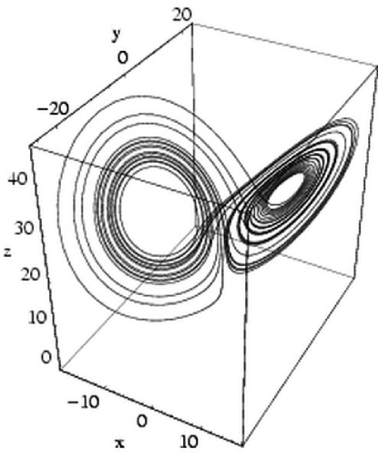
Figure 1: The Lorenz attractor. All initial conditions except the origin (which is an unstable equilibrium) are attracted to the figure shown.

II.1 The deviation vector method

The most straightforward method for calculating the largest Lyapunov exponent is to consider an initial point $\mathbf{y}^{(1)}_{0}=\mathbf{y}_{0}$ and a nearby point $\mathbf{y}^{(2)}_{0}=\mathbf{y}_{0}+\delta\mathbf{y}_{0}$, and then evolve both points forward, keeping track of the difference $\delta\mathbf{y}\equiv\mathbf{y}^{(2)}-\mathbf{y}^{(1)}$. If the motion is chaotic, then exponential separation implies that

$$\|\delta\mathbf{y}\|=e^{\lambda_{\mathrm{max}}t}\,\|\delta\mathbf{y}_{0}\|,$$ (4)

so that the largest exponent is

$$\lambda_{\mathrm{max}}=\frac{\log{[r_{e}(t)]}}{t},$$ (5)

where we write

$$r_{e}=\|\delta\mathbf{y}\|/\|\delta\mathbf{y}_{0}\|,$$ (6)

with a subscript $e$ that anticipates the ellipsoid axis discussed in Sec. II.2.3. Here $\|\cdot\|$ denotes the Euclidean norm (though in principle any positive-definite norm will do Eckmann and Ruelle (1985)). It is convenient to display the results of this process graphically by plotting $\log{[r_{e}(t)]}$ vs. $t$, which we refer to as a Lyapunov plot; since Eq. (5) is equivalent to $\log{[r_{e}(t)]}=\lambda_{\mathrm{max}}t$, such plots should be approximately linear, with slope equal to the principal Lyapunov exponent. (In practice, to extract the slope we perform a least-squares fit to the simulation data, which is less sensitive to fluctuations in the value of $\log{[r_{e}(t)]}$ than the ratio $\log{[r_{e}(t_{f})]}/t_{f}$ at the final time.) We refer to this technique as the (unrescaled) deviation vector method.

It is important to note that, because of the problem of saturation, Eq. (5) does not define a true Lyapunov exponent. In a chaotic system, any deviation $\delta\mathbf{y}_{0}$, no matter how small, will eventually saturate, i.e., it will grow so large that it no longer represents the local behavior of the dynamical system. Moreover, chaotic systems are bounded by definition [in order to eliminate trivial exponential separation of the form $x(t)=x_{0}\,e^{\lambda t}$], so there is some bound $B$ on the distance between any two trajectories. As a result, in the infinite time limit Eq. (5) gives

$$\lambda_{\mathrm{max}}=\lim_{t\rightarrow\infty}\frac{\log{\|\delta\mathbf{y}\|/\|\delta\mathbf{y}_{0}\|}}{t}\leq\lim_{t\rightarrow\infty}\frac{\log{B/\|\delta\mathbf{y}_{0}\|}}{t}=0.$$ (7)

In the naïve unrescaled deviation vector method, the calculated exponent is always zero because of saturation.

One solution to the saturation problem is to rescale the deviation once it grows too large. For example, suppose that we set $\|\delta\mathbf{y}_{0}\|=\epsilon$ for some small $\epsilon$ (say $10^{-8}$), and then allow the deviation to grow by at most a factor of $f$. Then, whenever $\|\delta\mathbf{y}\|\geq f\,\|\delta\mathbf{y}_{0}\|$, we rescale the deviation back to a size $\epsilon$ and record the length $R_{i}=\|\delta\mathbf{y}\|/\|\delta\mathbf{y}_{0}\|$ of the expanded vector. If we perform $N$ such rescalings in the course of a calculation, the total expansion of the initial vector is then

$$r_{e}=\frac{\|\delta\mathbf{y}_{f}\|}{\|\delta\mathbf{y}_{0}\|}\prod_{i=1}^{N}R_{i},$$ (8)

where $\delta\mathbf{y}_{f}$ is the final size of the (rescaled) separation vector. Applying Eq. (5), we see that the approximate Lyapunov exponent satisfies

$$\lambda_{\mathrm{max}}=\frac{1}{t}\left[\log{\left(\frac{\|\delta\mathbf{y}_{f}\|}{\|\delta\mathbf{y}_{0}\|}\right)}+\sum_{i=1}^{N}\log{R_{i}}\right].$$ (9)

We refer to this as the (rescaled) deviation vector method.

The rescaled deviation vector method is not particularly robust compared to the rigorous method described below (Sec. II.2), and there are significant complications when applying it to constrained systems, but if implemented with care it provides a fast and accurate estimate for the largest Lyapunov exponent. Fig. 2 shows both the rescaled and unrescaled deviation vector methods applied to the Lorenz system [Eq. (II)]. Note in particular the saturation of the unrescaled approach. We discuss the limitations of the rescaled method further in Sec. IV.

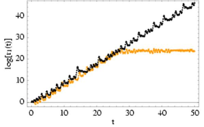
Figure 2: Comparison of the unrescaled (light) and rescaled (dark) deviation vector methods for calculating the principal Lyapunov exponent of the Lorenz system [Eq. (II)]. The slope of the rescaled line is the Lyapunov exponent ($\lambda_{\mathrm{max}}=0.905\pm 0.003$; see Sec. II.4.1). The initial deviation is $\|\delta\mathbf{y}_{0}\|=10^{-8}$, and rescaling occurs (for the rescaled method) if $\|\delta\mathbf{y}\|\geq 10^{-2}$. Note the saturation of the unrescaled approach once the deviation has grown too large.

II.2 The Jacobian method

Although the deviation vector method suffices for practical calculation in many cases, in essence it amounts to taking a numerical derivative. For a one-dimensional function of one variable, we can approximate the derivative at $x=x_{0}$ using

$$f^{\prime}(x_{0})\approx\frac{f(x_{0}+\epsilon)-f(x_{0})}{\epsilon},$$ (10)

for some $\epsilon\ll 1$, but this prescription is notoriously inaccurate as a numerical calculation Press et al. (1992). Of course, it is better (if possible) to calculate the analytical derivative $f^{\prime}(x)$ and evaluate it at $x_{0}$. The higher-dimensional generalization of this is the Jacobian matrix, which describes the local (linear) behavior of a higher-dimensional function. In the context of a dynamical system, this means that we can find the time-evolution of a small deviation $\delta\mathbf{y}$ using the rigorous linearization of the equations of motion:

$$\mathbf{f}(\mathbf{y}+\delta\mathbf{y})-\mathbf{f}(\mathbf{y})=\mathbf{Df}\cdot\delta\mathbf{y}+O(\|\delta\mathbf{y}\|^{2}),$$ (11)

where

$$(\mathbf{Df})_{ij}=\frac{\partial f_{i}}{\partial x^{j}}$$ (12)

is the Jacobian matrix evaluated along the flow. For example, for the Lorenz system [Eq. (II)] we have

$$\mathbf{Df}=\left(\begin{array}[]{ccc}-\sigma&\sigma&0\\ r-z(t)&-1&-x(t)\\ y(t)&x(t)&-b\\ \end{array}\right),$$ (13)

where we write the coordinates as functions of time to emphasize that Eq. (13) is different at each time $t$.

II.2.1 Jacobian diagnostic

One note about Jacobian matrices is worth mentioning: practical experience has shown that errors occasionally creep into the calculations leading to the Jacobian matrix, especially if the equations of motion are complicated. It is therefore worthwhile to note that Eq. (11) provides an invaluable diagnostic: calculate the quantity

$$\Delta=\mathbf{f}(\mathbf{y}+\delta\mathbf{y})-\mathbf{f}(\mathbf{y})-\mathbf{Df}\cdot\delta\mathbf{y}$$ (14)

for varying values of $\|\delta\mathbf{y}\|$; if $\Delta$ does not generally scale as $\|\delta\mathbf{y}\|^{2}$, then something is amiss. (The routines in Hartl include this important Jacobian diagnostic function.)

II.2.2 The principal exponent

The main value of Eq. (11) in the context of a dynamical system is its combination with Eq. (2) to yield an equation of motion for the deviation $\delta\mathbf{y}$:

$$\mathbf{f}(\mathbf{y}+\delta\mathbf{y})=\frac{d}{dt}(\mathbf{y}+\delta\mathbf{y})=\mathbf{f}(\mathbf{y})+\frac{d(\delta\mathbf{y})}{dt},$$ (15)

so that (discarding terms higher than linear order) Eq. (11) gives

$$\frac{d(\delta\mathbf{y})}{dt}=\mathbf{Df}\cdot\delta\mathbf{y}.$$ (16)

This equation is only approximately true for finite (that is, non-infinitesimal) deviations, but we can take the infinitesimal limit by identifying the deviation $\delta\mathbf{y}$ with an element $\bm{\xi}$ in the tangent space at $\mathbf{y}$. This leads to an exact equation for $\bm{\xi}$:

$$\frac{d\bm{\xi}}{dt}=\mathbf{Df}\cdot\bm{\xi}.$$ (17)

The initial value of $\bm{\xi}$ is arbitrary, but it is convenient to require that $\|\bm{\xi}_{0}\|=1$, so that the factor by which $\bm{\xi}$ has grown at some later time $t$ is simply $\|\bm{\xi}(t)\|$.

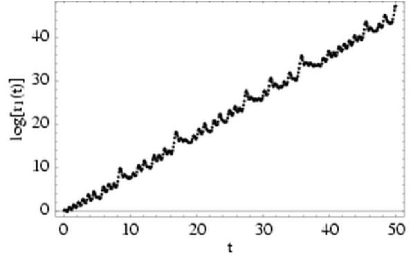
Figure 3: The natural logarithm of the tangent vector length $r_{1}\equiv\|\bm{\xi}(t)\|$ vs. $t$ for the Lorenz system. The slope of the rescaled line is the system’s largest Lyapunov exponent ($\lambda_{\mathrm{max}}\approx 0.905$). The figure and exponent are virtually identical to the rescaled deviation method show in Fig. 2.

The core of the Jacobian method for the principal Lyapunov exponent is to solve Eqs. (2) and (17) as a coupled set of differential equations. As in Sec. II.1, for chaotic systems the length of the deviation vector will grow exponentially, so that

$$\|\bm{\xi}(t)\|\approx e^{\lambda_{\mathrm{max}}t},$$ (18)

which implies that

$$\lambda_{\mathrm{max}}=\frac{\log{\|\bm{\xi}(t)\|}}{t}.$$ (19)

For sufficiently large values of $t$, Eq. (19) provides an approximation for the largest Lyapunov exponent. It is essential to understand that there is no restriction on the length of the tangent vector $\bm{\xi}$: the Jacobian method does not saturate. The only limitation on the size of $\bm{\xi}$ in practice is the maximum representable floating point number on the computer.

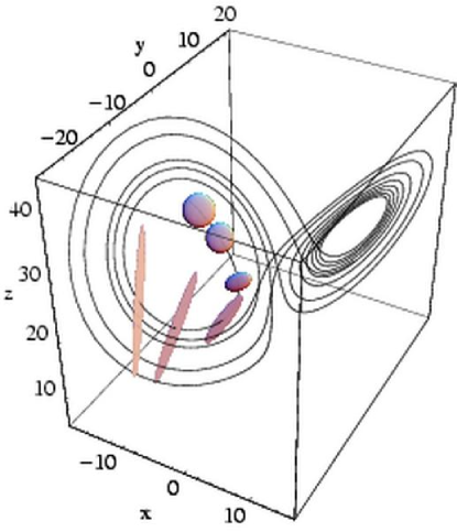
Figure 4: The Lorenz system with an evolving ellipsoid. The ellipsoid is calculated exactly in the tangent space (for a total time $t=0.4$) and is superposed on the phase space for the purposes of visualization. There is one expanding axis ($\sim e^{0.905\,t}$) and one contracting axis ($\sim e^{-14.57\,t}$); the third axis has a fixed unit length (Sec. II.4.1).

II.2.3 Ellipsoids and multiple exponents

Although following the time-evolution of a tangent vector $\bm{\xi}$ in place of a finite deviation $\delta\mathbf{y}$ solves the problem of saturation, it still only allows us to determine the principal exponent $\lambda_{\mathrm{max}}$. For a system with $n$ degrees of freedom, this leaves $n-1$ exponents undetermined. In order to calculate all $n$ exponents, we must introduce $n$ tangent vectors. (We discuss the value of knowing all $n$ exponents in Sec. II.3 below.) Since $n$ (linearly independent) vectors span an $n$-dimensional ellipsoid, this leads to a visualization of the Lyapunov exponents in terms of the evolution of a tangent space ellipsoid (Fig. 4). Fig. 5 shows the corresponding Lyapunov plot.

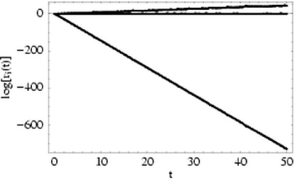
Figure 5: The natural logarithms of all three of the ellipsoid axes $r_{i}$ vs. $t$ for the Lorenz system, calculated using the Jacobian method (Sec. II.2). The slopes are the Lyapunov exponents. The three lines correspond to the exponents $\lambda_{1}\approx 0.905$, $\lambda_{2}\approx 0.0$, and $\lambda_{3}\approx-14.57$ (Sec. II.4.1). These values agree with the calculations in Alligood et al. (1997).

The general method is to introduce a linearly independent set of vectors $\{\bm{\xi}^{(1)},\bm{\xi}^{(2)},\ldots,\bm{\xi}^{(n)}\}$. It is convenient to begin the integration with vectors that form the orthogonal axes of a unit ball, so that the vectors $\{\bm{\xi}^{(1)}_{0},\bm{\xi}^{(2)}_{0},\ldots,\bm{\xi}^{(n)}_{0}\}$ are orthonormal. Each of these tangent vectors satisfies its own version of Eq. (17):

$$\frac{d\bm{\xi}^{(n)}}{dt}=\mathbf{Df}\cdot\bm{\xi}^{(n)}.$$ (20)

If we combine the $n$ tangent vectors to form the columns of a matrix $\mathbf{U}$, then Eq. (20) implies that

$$\frac{d\mathbf{U}}{dt}=\mathbf{Df}\cdot\mathbf{U}.$$ (21)

This equation, combined with Eq. (2), describes the evolution of a unit ball into an $n$-dimensional ellipsoid.

The value of the tangent space ellipsoid is this: if $r_{i}$ is the $i$th principal ellipsoid axis [and $r_{i}(0)=1$], then

$$r_{i}(t)=e^{\lambda_{i}t},$$ (22)

where $\lambda_{i}$ is the $i$th Lyapunov exponent. That is, the ellipsoid’s axes grow (or shrink) exponentially, and if $\lambda_{i}>0$ for any $i$ then the system is chaotic Eckmann and Ruelle (1985). [Recall that we refer to the semiaxes as “axes” for brevity (Sec. I).] Turning Eq. (22) around, we can find the $i$th Lyapunov exponent by finding the average stretching (or shrinking) per unit time of the $i$th principal ellipsoid axis:

$$\lambda_{i}\approx\frac{\log{[r_{i}(t)]}}{t}.$$ (23)

In practice, a more robust prescription is to record $\log{[r_{i}(t)]}$ as a function of $t$ and perform a least-squares fit to the pairs $(t_{j},\log{[r_{i}(t_{j})]})$ to find the slope $\lambda_{i}$.

Though Eq. (23) provides an estimate for the $i$th Lyapunov exponent, it requires us to find the $n$ principal axes of the final ellipsoid. While it is true that the columns of the final matrix $\mathbf{U}_{f}$ necessarily span an ellipsoid, but they are not in general orthogonal; in particular, the final tangent vectors do not necessarily coincide with the ellipsoid’s principal axes. A first step in extracting these axes is to note an important theorem in linear algebra (see Alligood et al. (1997) for a proof):

Theorem 1

Let $A$ be an $n\times n$ real matrix consisting of $n$ linearly independent column vectors $\{\mathbf{v}_{i}\}_{i=1}^{n}$, and let $\{s_{i}^{2}\}_{i=1}^{n}$ be the eigenvalues and $\{\mathbf{u}_{i}\}_{i=1}^{n}$ the normalized eigenvectors of $A^{T}A$ (where $A^{T}$ is the transpose of $A$). Then $\{\mathbf{v}_{i}\}_{i=1}^{n}$ lie on an $n$-dimensional ellipsoid whose principal axes are $\{s_{i}\,\mathbf{u}_{i}\}_{i=1}^{n}$.

In other words, finding the principal axes of the ellipsoid represented by a matrix $A$ is equivalent to finding the eigensystem of $A^{T}A$. (We note that the ellipsoid is unique: any other matrix $B$ whose columns $\{\mathbf{w}_{i}\}_{i=1}^{n}$ lie on the same ellipsoid as $\{\mathbf{v}_{i}\}_{i=1}^{n}$ must necessarily give the same principal axes.)

In principle, we are done: simply evolve $\mathbf{U}$ for a long time, and find the eigenvalues of $\mathbf{U}^{T}\mathbf{U}$. In practice, this fails miserably; every (generic) initial vector $\bm{\xi}^{(i)}_{0}$ has some component along the direction of greatest stretching, so all initial tangent space vectors eventually point approximately along the longest principal axis. As a result, all axes but the longest one are lost due to finite floating point precision.

The solution is to find new orthogonal axes as the system evolves. In other words, we can let the system evolve for some time $T$, stop to calculate the principal axes of the evolving ellipsoid, and then continue the integration. The method we advocate is the Gram-Schmidt orthogonalization procedure, which results in an orthogonal set of vectors spanning the same volume as the original ellipsoid, and with directions that converge to the true ellipsoid axes. This approach, originally described in Benettin et al. (1980), is a common textbook approach Alligood et al. (1997); Ott (1993), and was used successfully by the present author in Hartl (2003a). Numerically, the Gram-Schmidt algorithm is subject to considerable roundoff error Press et al. (1992), and is usually considered a poor choice for orthogonalizing vectors, but in the context of dynamics its performance has proven to be astonishingly robust. (See Sec. IV for further discussion.)

We review briefly the Gram-Schmidt construction, and then indicate its use in calculating Lyapunov exponents. Given $n$ linearly-independent vectors $\{{\bf u}_{i}\}$, the Gram-Schmidt procedure constructs $n$ orthogonal vectors $\{{\bf v}_{i}\}$ that span the same space, given by

$${\bf v}_{i}={\bf u}_{i}-\sum_{j=1}^{i-1}\frac{{\bf u}_{i}\cdot{\bf v}_{j}}{\|{\bf v}_{j}\|^{2}}\,{\bf v}_{j}.$$ (24)

To construct the $i$th orthogonal vector, we take the $i$th vector from the original set and subtract off its projections onto the previous $i-1$ vectors produced by the procedure. The use of Gram-Schmidt in dynamics comes from observing that the resulting vectors approximate the axes of the tangent space ellipsoid. After the first time $T$, all of the vectors point mostly along the principal expanding direction. We may therefore pick any one as the first vector in the Gram-Schmidt algorithm, so choose $\bm{\xi}_{1}\equiv{\bf u}_{1}$ without loss of generality. If we let ${\bf e}_{i}$ denote unit vectors along the principal axes and let $r_{i}$ be the lengths of those axes, the dynamics of the system guarantees that the first vector ${\bf u}_{1}$ satisfies

$${\bf u}_{1}=r_{1}{\bf e}_{1}+r_{2}{\bf e}_{2}+\cdots\approx r_{1}{\bf e}_{1}\equiv{\bf v}_{1}$$

since ${\bf e}_{1}$ is the direction of fastest stretching. The second vector ${\bf v}_{2}$ given by Gram-Schmidt is then

$${\bf v}_{2}={\bf u}_{1}-\frac{{\bf u}_{1}\cdot{\bf v}_{1}}{\|{\bf v}_{1}\|^{2}}\,{\bf v}_{1}\approx{\bf u}_{1}-r_{1}{\bf e}_{1}=r_{2}{\bf e}_{2},$$

with an error of order $r_{2}/r_{1}$. The procedure proceeds iteratively, with each successive Gram-Schmidt step (approximately) subtracting off the contribution due to the previous axis direction. In principle, the system should be allowed to expand to a point where $r_{2}\ll r_{1}$, but (amazingly) in practice the Gram-Schmidt procedure converges to accurate ellipsoid axes even when the system is orthogonalized and even normalized on timescales short compared to the Lyapunov stretching timescale. As a result, the procedure below can be abused rather badly and still give accurate results (Sec. IV).

II.2.4 The algorithm in detail

We summarize here the method used to calculate all the Lyapunov exponents of an unconstrained dynamical system $\dot{\mathbf{y}}=\mathbf{f}(\mathbf{y})$ with $n$ degrees of freedom:

1. Construct an orthonormal matrix $\mathbf{U}_{0}$ whose columns (the initial tangent vectors) span a unit ball, and then integrate

   $$\dot{\mathbf{y}}=\mathbf{f}(\mathbf{y})$$ (25)

   and

   $$\dot{\mathbf{U}}=\mathbf{Df}\cdot\mathbf{U}$$ (26)

   as a coupled set of $2n$ differential equations. We recommend choosing a random initial ball for genericity.

2. At various times $t_{j}$, replace $\mathbf{U}$ with the orthogonal axes of the ellipsoid defined by $\mathbf{U}$, using the Gram-Schmidt orthogonalization procedure. This can be done either every time $T$, for some suitable choice of $T$, or every time the integrator takes a step. We have found the latter prescription to be especially robust in practice.

3. If the length of any axis exceeds some very large value (say, near the maximum representable floating point value), normalize the ellipsoid and record the axis lengths

   $$R_{i}^{(k)}\qquad\mbox{($i$th axis at $k$th rescaling)}$$ (27)

   at the rescaling time. Do the same if any axis is smaller than some very small number.

4. Record the value of

   $$\log{r_{i}^{(j)}}=\log{[L_{i}(t_{j})]}+\sum_{k=1}^{k_{\mathrm{max}}}\log{R_{i}^{(k)}}$$ (28)

   at each time $t_{j}$, where $L_{i}$ is the $i$th principal axis length. The second term accounts for the axis lengths at the $k_{\mathrm{max}}$ rescaling times. Note that if $t_{j}$ is a rescaling time itself, then $\log{[L_{i}(t_{j})]}=\log{1}=0$, since by construction the ellipsoid has been normalized back to a unit ball.

5. After reaching the final number of time steps $N$, perform a least squares fit on the pairs $(t_{j},\log{r_{i}^{(j)}})$ to find the slopes $\lambda_{i}$. Since

   $$\log{[r_{i}(t)]\approx\lambda_{i}t},$$ (29)

   the slope $\lambda_{i}$ is the Lyapunov exponent corresponding to the $i$th principal axis. Using the Gram-Schmidt procedure should result in the relationship $\lambda_{1}>\ldots>\lambda_{n}$.

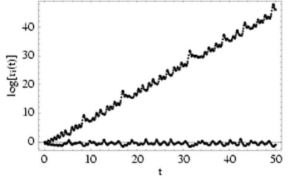
Figure 6: Close-up of Fig. 5, showing the natural logarithms of the two largest ellipsoid axes vs. $t$ for the Lorenz system, calculated using the Jacobian method (Sec. II.2). The slopes are the Lyapunov exponents. The plot for the larger axis closely matches the figures for the rescaled deviation vector method (Fig. 2) and the single tangent vector Jacobian method (Fig. 3).

Most of the value of calculating $\lambda_{i}$ for $i>1$ comes from having all $n$ of the exponents (Sec. II.3 below). Nevertheless, it is worth noting that the algorithm works for any value $0<m\leq n$, so the method above can be used without alteration to find an arbitrary number of exponents. Fig. 6 shows the axis growth for $m=2$ in the Lorenz system, while Fig. 5 shows the growth for $m=n=3$.

II.3 The value of multiple exponents

Calculating all the exponents of a system of differential equations allows us to paint a more complete picture of the dynamics in several different ways. In particular, with all $n$ exponents comes the ability to visualize the entire phase space ellipsoid (instead of just its principal axis), as in Fig. 4. Another important benefit of knowing all the exponents is a determination of dissipative or conservative behavior. Conservative flows preserve phase space volumes, while dissipative flows contract volumes. Geometrically, the volume $V$ of an ellipsoid is proportional to the product of its principal axes $\{r_{i}\}$, so that the ratio of the final to the initial volume is

$$\frac{V_{f}}{V_{0}}=\prod_{i}r_{i},$$ (30)

assuming that the initial volume is a unit ball. For dissipative systems, phase space volumes in general contract exponentially according to

$$\frac{V_{f}}{V_{0}}=e^{-\Lambda t},$$ (31)

where $\Lambda$ is a positive constant. Combining Eq. (30) and Eq. (31) yields

$$\Lambda=-\log{\left(\frac{V_{f}}{V_{0}}\right)}=-\log{\left(\prod_{i}r_{i}\right)}=-\sum_{i}\log{r_{i}}=-\sum_{i}\lambda_{i},$$ (32)

where the $\lambda_{i}$ are the Lyapunov exponents. In other words, the phase space volume contraction constant $\Lambda$ is equal to minus the sum of the Lyapunov exponents.

If the Lyapunov exponents sum to zero, then the contraction factor vanishes, and volumes are conserved—i.e, the system is conservative. The special case of Hamiltonian systems is of particular interest, since the equations of motion for many mechanical systems can be derived from a Hamiltonian. The Hamiltonian property strongly constrains the Lyapunov exponents, which must cancel pairwise: to each exponent $+\lambda$ there corresponds a second exponent $-\lambda$ Eckmann and Ruelle (1985). Several examples of this $\pm\lambda$ property of Hamiltonian systems appear below.

Having all the Lyapunov exponents also allows us to verify that there is at least one vanishing exponent, corresponding to motion tangent to the flow, which must be the case for any chaotic system. (See Ref. Alligood et al. (1997) for a proof.) Since we have finite numerical precision, we do not expect to find any exponent to be identically zero, but some exponent should always be close to zero. A practical criterion for “close to zero” is to compute error estimates for the least-squares fits advocated in Sec. II.2.4; an exponent is “close to zero” if it is zero to within the standard error of the fit. Applications of this method appear in Sec. II.4.1 and Sec. II.4.2 below. It is worth noting that the fitting errors are not the dominant source of variance in calculating Lyapunov exponents; variations in the initial conditions and initial deviation vectors contribute more to the uncertainty than errors in the fits. See Sec. II.4.1 for further discussion.

One final note deserves mention: the statement that $\Lambda=-\sum_{i}\lambda_{i}$ is equivalent to a theorem due to Liouville Alligood et al. (1997), which relates the volume contraction to the trace of the Jacobian matrix:

$$\frac{V_{f}}{V_{0}}=\exp{\left(\int_{0}^{t}\mathrm{Tr}\,\mathbf{Df}(t)\,dt\right)},$$ (33)

where again we assume that $V_{0}$ corresponds to a unit ball. If the trace of the Jacobian matrix happens to be time-independent, then this yields

$$\frac{V_{f}}{V_{0}}=\exp{\left[(\mathrm{Tr}\,\mathbf{Df})\,t\right]},\qquad\mbox{(time-independent trace)}$$ (34)

so that Eq. (32) gives $\Lambda=-\mathrm{Tr}\,\mathbf{Df}$. In this special case, we can perform a consistency check by verifying that

$$\sum_{i}\lambda_{i}=\mathrm{Tr}\,\mathbf{Df}.\qquad\mbox{(time-independent trace)}$$ (35)

II.4 Examples

II.4.1 The Lorenz system

Following the phase space ellipsoid allows us to visualize the dynamics of the Lorenz system in an unusual way. Fig. 4 shows the Lorenz attractor together with the phase space ellipsoid for a short amount of time ($t_{f}=0.4$). The initial ball is evolved using Eq. 21, so it represents the true tangent space evolution, which is then superposed on the Lorenz phase space $(x,y,z)$. It is evident that the initial ball is stretched in one direction and flattened in another, as well as rotated. (As we shall see, the third direction is neither stretched nor squeezed, corresponding to the zero exponent discussed in Sec. II.3.)

By recording natural logarithms of the ellipsoid axes as the system evolves, we can obtain numerical estimates for the Lyapunov exponents, as discussed in Sec. II.2.4. A plot of $\log{[r_{i}(t)]}$ vs. $t$ appears in Fig. 5 for a final time $t_{f}=50$, with the slopes giving approximate values for the exponents. Using a $t_{f}=5000$ integration for greater accuracy yields the estimates

$$\lambda_{1} = 0.905\pm 9\times 10^{-6}$$

$$\lambda_{2} = 1.5\times 10^{-6}\pm 1.7\times 10^{-6}$$ (36)

$$\lambda_{3} = -14.57\pm 9\times 10^{-6}$$

for the parameter values $\sigma=10$, $b=8/3$, and $r=28$. The $\pm$ values are the standard errors on the least-squares fit of $\log{[r_{i}(t)]}$ vs. $t$. One of the exponents is close to zero (as required for a flow) in the sense of Sec. II.3: the error in the fit not small compared to the exponent. [In the case shown in Eq. (II.4.1), the “error” is actually larger than the exponent.] The other two exponents are clearly nonzero, with the positive exponent indicating chaos.

As mentioned briefly in Sec. II.3, the largest source of variance in calculating Lyapunov exponents is variations in the initial conditions, not errors in the least-squares fits used to determine the exponents. We express the exponents in the form

$$\bar{\lambda}\pm\frac{\sigma}{\sqrt{N}},$$ (37)

where

$$\bar{\lambda}=\frac{1}{N}\,\sum_{j=1}^{N}\lambda^{(j)}$$ (38)

is the sample mean and

$$\sigma=\sqrt{\frac{1}{N-1}\,\sum_{j=1}^{N}\left(\lambda^{(j)}-\bar{\lambda}\right)^{2}}$$ (39)

is the standard deviation. For the Lorenz system, using a final integration time of $t_{f}=5000$ for $N=50$ random initial balls [all centered on the same initial value of $(x_{0},y_{0},z_{0})$] gives

$$\lambda_{1} = 0.9053\pm 4.1\times 10^{-4}$$

$$\lambda_{2} = -4.5\times 10^{-6}\pm 7.6\times 10^{-7}$$ (40)

$$\lambda_{3} = -14.5720\pm 4.1\times 10{-4}$$

The values of the error are much greater than the standard errors associated with the least-squares fit for the slope for any one trial. As expected, it is evident that $\lambda_{2}$ is consistent with zero.

There is a strongly expanding direction and a very strongly contracting direction in the Lorenz system, and the volume contraction constant $\Lambda$ is large: $\Lambda=-\sum_{i}\lambda_{i}=13.67$, so that after a time $t=5000$ the volume is an astonishingly small $6.75\times 10^{-29674}$. This is despite the exponential growth of the largest principal axis, which grows in this same time to a length $1.52\times 10^{1965}$; the volume nevertheless contracts, since the smallest axis shrinks to $4.44\times 10^{-31639}$ in the same time. We note that the periodic renormalization and reorthogonalization of the ellipsoid axes is absolutely essential from a numerical perspective, since these axis lengths are far above and below the floating point (double precision) limits of $\mathtt{xmax}\approx\mathtt{xmin^{-1}}\approx 10^{308}$ on a typical IEEE-compliant machine Press et al. (1992).

The Lorenz system affords an additional check on the numerically determined exponents: the trace of the Jacobian matrix [Eq. (13)] is time-independent, so the exponents should satisfy Eq. (35):

$$\sum_{i}\lambda_{i}=-13.67\stackrel{{\scriptstyle?}}{{=}}\mathrm{Tr}\,\mathbf{Df}=-(\sigma+1+b)=-\frac{41}{3}\approx-13.67.$$ (41)

Eq. (35) is thus well-satisfied.

II.4.2 The forced damped pendulum

We turn now to our second principal example of a chaotic dynamical system, the forced damped pendulum (FDP). This is a standard pendulum with damping and periodic forcing; written as a first-order ODE, our equations are as follows:

$$\dot{\theta} = \omega$$

$$\dot{\omega} = -c\,\omega-\sin\theta+\rho\,\sin t$$ (42)

$$\dot{t} = 1$$

Here $c$ is the damping coefficient and $\rho$ is the forcing amplitude, and the gravitational acceleration $g$ and pendulum length $\ell$ are set to one for simplicity. We include the equation $\dot{t}=1$ so that the system is autonomous (i.e., we remove the explicit time-dependence by treating time as a dynamical variable with unit time derivative). In addition to being an example with transparent physical relevance (in contrast to the Lorenz system), the forced damped pendulum, in slightly altered form, serves as a model constrained system in Sec. III below.

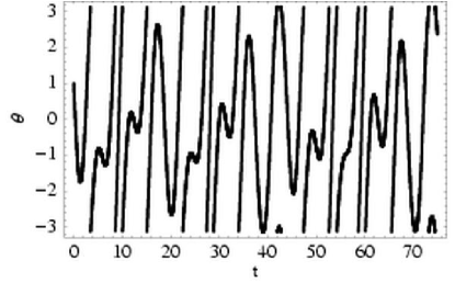
Figure 7: $\theta$ vs. $t$ for the forced damped pendulum [Eq. (II.4.2)].

The forced damped pendulum is chaotic for many values of $c$ and $\rho$. For simplicity, in the present case we fix $c=0.1$ and $\rho=2.5$. A plot of $\theta$ vs. $t$ shows the system’s erratic behavior (Fig. 7), but a more compelling picture of the dynamics comes from a time-$2\pi$ stroboscopic map. A time-$T$ map involves taking a snapshot of the system every time $T$ and then plotting $\omega$ vs. $\theta$. Since the forcing term in Eq. (II.4.2) is $2\pi$-periodic, this provides a natural value for $T$ in the present case. The resulting plot shows the characteristic folding and stretching of a fractal attractor (Fig. 8), which for the FDP attracts almost all initial conditions Alligood et al. (1997).

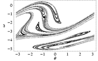
Figure 8: $\omega$ vs. $\theta$: the time-$2\pi$ stroboscopic map for the forced damped pendulum. A point $(\omega=\dot{\theta},\theta)$ is plotted every time $2\pi$, resulting in a fractal attractor characteristic of dissipative chaos.

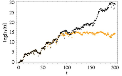
Figure 9: The natural logarithms of all three of the ellipsoid axes $r_{i}$ vs. $t$ for the forced damped pendulum, calculated using the Jacobian method (Sec. II.2). The slopes are the Lyapunov exponents. The three lines correspond to the exponents $\lambda_{1}=0.160\pm 0.0049$, $\lambda_{2}=0.0$, and $\lambda_{3}=-0.262\pm 0.0053$ (Sec. IV and Table 1).

The forced damped pendulum is dissipative and strongly chaotic. We calculate the Lyapunov exponents (Fig. 9) using the Jacobian matrix:

$$\mathbf{Df}=\left(\begin{array}[]{ccc}0&1&0\\ -\cos\theta&~{}~{}-c{}{}&\rho\cos t\\ 0&0&0\\ \end{array}\right),$$ (43)

The Lyapunov exponents are (for a $t_{f}=5\times 10^{4}$ integration)

$$\lambda_{1} = 0.160\pm 7\times 10^{-6}$$

$$\lambda_{2} = 8\times 10^{-8}\pm 1\times 10^{-7}$$ (44)

$$\lambda_{3} = -0.262\pm 7\times 10^{-6}$$

where the error terms are the standard errors in the least-squares fit for the slope. (See Sec. IV and especially Table 1 for the true errors due to varying initial deviations.) One exponent is consistent with zero (as required for a flow) to within the error of the fit. The dissipation constant is $\Lambda=-\sum_{i}\lambda_{i}=0.1$. The trace of the Jacobian matrix is time-independent, so that $\mathrm{Tr}\,\mathbf{Df}=-c$, and indeed $\sum_{i}\lambda_{i}=-0.1=-c=\mathrm{Tr}\,\mathbf{Df}$ as predicted by Eq. 35.

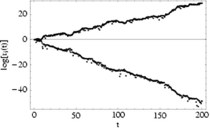
Figure 13: The natural logarithms of both ellipsoid axes for the constrained forced damped pendulum, calculated using the restricted Jacobian method (Sec. III.3). The slopes are the Lyapunov exponents. The results agree well with the unconstrained case (Fig. 9 and Table 1).

The zero exponent in the FDP is associated with the time “degree of freedom” in the Jacobian: if we delete the final row and column of the Jacobian matrix, only the positive and negative exponents remain (see, e.g., Fig. 13 below). Since the time is not an actual dynamical variable, for the remainder of this paper we will suppress this “time piece,” but it is important to note that the time dependence is absolutely crucial to the presence of chaos. According to the Poincaré-Bendixon theorem Alligood et al. (1997), an autonomous system of differential equations with fewer than three degrees of freedom cannot be chaotic. We will treat the FDP system as a time-dependent system with two degrees of freedom, but the extra equation $\dot{t}=1$ in the autonomous formulation is what creates the potential for chaos.

An instructive case to consider is the limit $c=\rho=0$. In this limit, the system is a simple pendulum, which is a Hamiltonian system. A simple pendulum is not chaotic, of course, and both its Lyapunov exponents are zero, but the Hamiltonian character of the system nevertheless shows up in the $\pm\lambda$ property discussed above (Sec. II.3): numerically, the exponents approach zero in a symmetric fashion, as shown in Fig. 10.

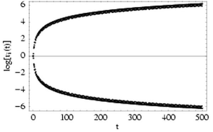
Figure 10: The natural logarithms of the ellipsoid axes $r_{i}$ vs. $t$ for the forced damped pendulum in the limit of zero dissipation and zero forcing (i.e., a simple pendulum). The Lyapunov exponents are zero, and the distance between nearby trajectories grows linearly (leading to logarithmic growth in this log plot). Nevertheless, the Hamiltonian character of the system is manifest in the $\pm\lambda$ symmetry: for each exponent $+\lambda$, there is a corresponding exponent $-\lambda$. In the nonchaotic limiting case shown here, the Lyapunov exponents approach zero symmetrically.

III Lyapunov exponents in constrained flows

We come now to the raison d’être of this paper, namely, the calculation of Lyapunov exponents for constrained systems. For pedagogical purposes, our primary example is the forced damped pendulum with the position written in Cartesian coordinates. In addition to this instructive example, we also discuss two constrained systems of astrophysical interest, involving the orbits of spinning compact objects such as neutron stars or black holes (see, e.g., Hartl (2003a) and Hartl (2003b) and references therein).

Written in terms of the Cartesian coordinates $(x,y)=(\cos\theta,\sin\theta)$, the equations of motion for the FDP [Eq. (II.4.2)] become (upon suppressing the time piece)

$$\dot{x} = -\omega y$$

$$\dot{y} = \omega x$$ (45)

$$\dot{\omega} = -c\,\omega-y+\rho\,\sin t$$

For a pendulum with unit radius, the Cartesian coordinates of the pendulum satisfy the constraint

$$x^{2}+y^{2}=1.$$ (46)

Although it is certainly possible to use $(\dot{x},\dot{y})$ in the equations of motion, along with $(x,y)$, this is an unnecessary complication; in order to keep the equations as simple as possible, we retain the variable $\omega$ in the equations of motion.

Developing the techniques for solving constrained systems using this toy example has several advantages. The equations of motion and the constraint are extremely simple, which makes it easy to see the differences between the constrained and unconstrained cases. In addition, the constraint is easy to visualize, and yet it captures the key properties of much more complicated constraints. Finally, since we have already solved the same problem in unconstrained form, it is easy to verify that the techniques of this section reproduce the results from Sec. II.4.2.

III.1 Constraint complications

To see how constraints complicate the calculation of Lyapunov exponents, consider an implementation of the deviation vector approach (Sec. II.1). In the unconstrained forced damped pendulum, given an initial condition, we would construct a deviated trajectory separated by a small angle $\delta\theta$ (and a small velocity $\delta\omega$). In the constrained version, a naïve implementation would use a deviated trajectory with spatial coordinates $x+\delta x$ and $y+\delta y$, where $\delta\mathbf{y}=(\delta x,\delta y)$ is a small but otherwise arbitrary deviation vector. But the deviations are not independent; the deviated initial condition must satisfy the constraint:

$$(x+\delta x)^{2}+(y+\delta y)^{2}=1.$$ (47)

To lowest order in $\delta x$, we must have $\delta y=-(x/y)\,\delta x$.

We can now consider a more general case. Suppose there are $k$ constraints, which we write as a $k$-dimensional vector equation $\mathbf{C}(\mathbf{y})=\mathbf{0}$. (In our example, $\mathbf{C}$ has only one component: with $\mathbf{y}=(x,y,\omega)$, we have $C_{1}(\mathbf{y})=x^{2}+y^{2}-1=0$.) Then if a point $\mathbf{y}$ satisfies the constraints, the deviated trajectory must satisfy them as well:

$$\mathbf{C}(\mathbf{y}+\delta\mathbf{y})=\mathbf{0}.$$ (48)

We will refer such a $\delta\mathbf{y}$ as a constraint-satisfying deviation.

Let us outline one possible method for constructing such a constraint-satisfying deviation. Let $n$ be the number of phase space coordinates ($n=3$ for the constrained forced damped pendulum model). Consider an $n$-dimensional vector $\tilde{\mathbf{y}}_{0}$ that has $d$ nonzero entries, where $d$ represents the true number of degrees of freedom ($d=2$ for the constrained FDP). Assume that we have some method for constructing from $\tilde{\mathbf{y}}_{0}$ an $n$-dimensional initial condition $\mathbf{y}_{0}$ that satisfies the constraints. For example, we could specify the initial values of $x$ and $\omega$, and then derive an initial value of $y$ using $y=\sqrt{1-x^{2}}$ (or $y=-\sqrt{1-x^{2}}$; more on this later). Now consider an $n$-dimensional vector $\tilde{\mathbf{y}}^{\prime}_{0}=\tilde{\mathbf{y}}_{0}+\delta\tilde{\mathbf{y}}_{0}$, which adds arbitrary deviations to $d$ degrees of freedom. We can then use the same method as above to find $\mathbf{y}^{\prime}_{0}$ from $\tilde{\mathbf{y}}^{\prime}_{0}$, and then set

$$\delta\mathbf{y}_{0}=\mathbf{y}^{\prime}_{0}-\mathbf{y}_{0}$$ (49)

to arrive at a constraint-satisfying deviation.

Figure 11: Comparison of the unrescaled (light) and rescaled (dark) constrained deviation vector methods for calculating the principal Lyapunov exponent of the constrained forced damped pendulum (Sec. III.2.1). The slope of the rescaled line is the Lyapunov exponent, $\lambda_{1}=0.161\pm 0.0046$ (Sec. IV). The initial deviation is $\|\delta\mathbf{y}_{0}\|=10^{-6}$, and rescaling occurs (for the rescaled method) if $\|\delta\mathbf{y}\|\geq 10^{-2}$, which happens 4 times in this figure. As in Fig. 2, the unrescaled approach saturates once the deviation has grown too large.

III.2 Constrained deviation vectors

Having determined $\delta\mathbf{y}_{0}$ by Eq. (49) (or by some other method), we can immediately apply the unrescaled deviation vector approach: simply track $\mathbf{y}^{\prime}$ and $\mathbf{y}$ as the two trajectories evolve, and monitor the length of $\delta\mathbf{y}=\mathbf{y}^{\prime}-\mathbf{y}$. Since the equations of motion preserve the constraint, the resulting $\delta\mathbf{y}$ is always constraint-satisfying. The only subtlety is using a restricted norm to eliminate the extra degrees of freedom; for example, the restricted FDP norm is

$$\|\delta\mathbf{y}\|_{r}=\sqrt{\delta x^{2}+\delta\omega^{2}}$$ (50)

if we choose to eliminate the $y$ degree of freedom. Since $\delta y\approx-(x/y)\,\delta x$, using the full Euclidean distance would add the term $\delta y^{2}=(x^{2}/y^{2})\,\delta x^{2}$ to the expression under the square root, leading to an overestimate for the principal exponent. The restricted norm avoids this problem by considering only true degrees of freedom.

III.2.1 Rescaling for constrained systems

In contrast to the simplicity of the unrescaled method, the rescaled deviation vector method requires great care, since a carelessly rescaled deviation is not constraint-satisfying: $\mathbf{C}(\mathbf{y}+\delta\mathbf{y}/r)\neq\mathbf{0}$ for a rescaling factor $r\neq 1$. In this case, it is necessary to extract $\delta\tilde{\mathbf{y}}$ from $\delta\mathbf{y}$ and then rescale it back to its initial size $\|\delta\tilde{\mathbf{y}}_{0}\|$ using the restricted norm. By reapplying the procedure leading to Eq. (49), we then find a new (rescaled) constraint-satisfying $\delta\mathbf{y}$ that satisfies $\|\delta\mathbf{y}\|_{r}=\|\delta\tilde{\mathbf{y}}_{0}\|$. In this case, it is essential that the new deviation vector have the same constraint branches as the old one. For example, suppose that in the FDP case the value of $y$ is negative before the rescaling. When calculating a new $\mathbf{y}^{\prime}$ to arrive at the rescaled deviation $\delta\mathbf{y}$, it is then essential to choose the negative branch in the equation $y^{\prime}=\pm\sqrt{1-x^{\prime 2}}$. The result of implementing this constrained deviation vector method to the forced damped pendulum appears in Fig. 11.

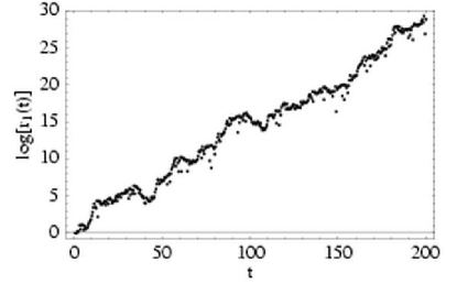
Figure 12: The natural logarithm of the tangent vector length $r_{1}\equiv\|\bm{\xi}(t)\|_{r}$ vs. $t$ for the constrained forced damped pendulum, using a constraint-satisfying tangent vector (Sec. III.2.2). We use the restricted norm $\|\cdot\|_{r}$ to calculate phase space distances (see text). Compare to Fig. 9 (unconstrained Jacobian method) and Fig. 11 (constrained deviation vector method).

III.2.2 A Jacobian method for the largest exponent

The method outlined above for unrescaled deviation vectors leads to a remarkably simple implementation of the single tangent vector Jacobian method. Given a constraint-satisfying deviation $\delta\mathbf{y}_{0}$, set

$$\bm{\xi}_{0}=\delta\mathbf{y}_{0}/\|\delta\mathbf{y}_{0}\|_{r},$$ (51)

where $\|\cdot\|_{r}$ is a restricted norm on the $d$ true degrees of freedom. We refer to such a $\bm{\xi}$ as a constraint-satisfying tangent vector. Since the equations of motion preserve the constraints, we can evolve this tangent vector using Eq. (17). The Jacobian method does not saturate, so we need only rescale if $\|\bm{\xi}\|_{r}$ approaches the floating point limit of the computer. We can then use a procedure based on the rescaled deviation method to find a new (rescaled) constraint-satisfying tangent vector, but this is typically unnecessary since by the time the floating point limit has been reached we already have a good estimate of the principal Lyapunov exponent. The resulting Lyapunov plot for the constrained FDP appears in Fig. 12.

III.2.3 Ellipsoid constraint complications

We now have three methods at our disposal for calculating the largest Lyapunov exponent, but for $d$ degrees of freedom there are $d$ exponents. What of these other exponents? Here we find an essential difficulty in implementing the ellipsoid method described in Sec. II.2.3. The core problem is this: the tangent vectors must be orthogonalized in order to extract all $d$ principal ellipsoid axes, but at the same time each tangent vector must be constraint-satisfying. Simply put, it is impossible in general to satisfy the requirements of orthogonality and constraint satisfaction simultaneously.

We present here two different solutions to this problem, which we will refer to as the restricted Jacobian method and the constrained ellipsoid method.

III.3 Restricted Jacobian method

The most natural response to a system with more coordinates $n$ than degrees of freedom $d$ is to eliminate the spurious degrees of freedom using the constraints. Unfortunately, this procedure is often difficult in practice: solving the constraint equations may involve polynomial or transcendental equations that have no simple closed form. Even for the simple case of the FDP, the sign ambiguity in $y=\pm\sqrt{1-x^{2}}$ makes a simple variable substitution impractical. Fortunately, such substitutions are unnecessary: since the equations of motion preserve the constraints, there is no need in general to eliminate $n-d$ coordinates. In fact, constraints can be a virtue, since they can be used to check the accuracy of the integration.

The same cannot be said of the Jacobian matrix. As argued above, the extra degrees of freedom lead to fundamental difficulties in applying the Jacobian method for finding Lyapunov exponents; constraints, far from being a virtue, are a considerable complication. In contrast to the equations of motion, though, it is relatively straightforward to eliminate the spurious degrees of freedom. The trick is to write a restricted $d\times d$ Jacobian matrix, with entries only for $d$ coordinates.

An example should make this clear. For the FDP system in constrained form, we wish to eliminate one degree of freedom in the Jacobian matrix, and we can choose to eliminate either $x$ or $y$. Choosing the latter, the Jacobian becomes

$$\mathbf{Df}=\left(\begin{array}[]{cc}\frac{\partial\dot{x}}{\partial x}&\frac{\partial\dot{x}}{\partial\omega}\\ \frac{\partial\dot{\omega}}{\partial x}&\frac{\partial\dot{\omega}}{\partial\omega}\\ \end{array}\right),$$ (52)

where we have suppressed the derivatives with respect to the “time degree of freedom” (as discussed in Sec. II.4.2). The term to focus on here is $\partial\dot{x}/\partial x$, which seems to be zero a priori since $\dot{x}=-\omega y$, but this is only true if we treat $x$ and $y$ as independent. Since we are eliminating the $y$ degree of freedom, we cannot treat them as independent; $y$ has a nonzero derivative with respect to $x$, so that

$$\frac{\partial\dot{x}}{\partial x}=-\omega\frac{\partial y}{\partial x}.$$ (53)

If we find $\partial y/\partial x$ using $y=\pm\sqrt{1-x^{2}}$, we have exactly the same sign ambiguity problem that we had in trying to eliminate the $y$ degree of freedom in the equations of motion. The difference here is the we need only the derivative of $y$, not an explicit solution for $y$ in terms of $x$, and this we can achieve by differentiating the constraint:

$$0=\frac{\partial}{\partial x}(x^{2}+y^{2})=2x+2y\frac{\partial y}{\partial x}\Rightarrow\frac{\partial y}{\partial x}=-\frac{x}{y}.$$ (54)

If we integrate the equations of motion using the variables $(x,y,\omega)$, then we have the value of $y$ at any particular time, and we never need deal with the sign ambiguity. Using the same trick to calculate $\partial\dot{\omega}/\partial x$, we can write the restricted Jacobian as

$$\mathbf{Df}=\left(\begin{array}[]{cc}\omega\,\displaystyle{\frac{x}{y}{}}&~{}-y\vskip 6.0pt plus 2.0pt minus 2.0pt\\ \displaystyle{\frac{x}{y}}&-c\\ \end{array}\right)$$ (55)

We now proceed exactly as in the unconstrained Jacobian method, using the restricted Jacobian to calculate the evolution of the initial tangent space ball. Since we deal only with a number of coordinates equal to the true number of degrees of freedom, the constraints are not a consideration, and we can reorthogonalize exactly as before.

The general case is virtually the same. For $n$ coordinates and $d$ degrees of freedom, there must be $m=n-d$ constraint equations of the form

$$C_{k}(\mathbf{y})=0$$ (56)

for $k=1\ldots m$. We must choose which $d$ coordinates to keep in the Jacobian matrix, eliminating $m$ coordinates in the process. By differentiating the constraints, we arrive at $m$ linear equations for the derivatives of the $m$ eliminated coordinates in terms of the $n$ variables:

$$\frac{\partial C_{k}}{\partial y_{j}}=0,$$ (57)

where $j$ ranges over the indices of the eliminated coordinates ($j=2$, corresponding to $y$, for the FDP). Since these are linear equations, they are both easy to solve and do not suffer from any sign or branch ambiguities. The $d\times d$ Jacobian matrices that result allow the calculation of Lyapunov exponents with all the robustness of the Jacobian method for unconstrained systems.

Figure 14: The orbit of a spinning relativistic binary, calculated using the post-Newtonian equations of motion. The equations model two spinning bodies, but we use an effective one-body approach to reduce the dynamics to the motion of one body. Distances are measured in terms of $GM/c^{2}$, where $M=m_{1}+m_{2}$ is the total mass of the system. For a pair of black holes, each with 10 times the mass of the Sun, the length unit is $GM/c^{2}=20\,GM_{\odot}/c^{2}=30\,\mathrm{km}$.

We considered the constrained forced damped pendulum for purposes of illustration, but it is admittedly artificial. A more realistic example is shown in Fig. 14, which illustrates the dynamics of two spinning black holes with comparable masses. (Such systems are of considerable interest for ground-based gravitational wave detectors such as the LIGO project.) The equations of motion come from the Post-Newtonian (PN) expansion of full general relativity—essentially, a series expansion in the dimensionless velocity $v/c$, where the first term is ordinary Newtonian gravity and the higher-order terms are post-Newtonian corrections (see, e.g., Damour (2001); Damour et al. (2000); Damour and Schäfer (1988)). The constraint comes from the spins of the black holes: it is most natural to think of the spin as having two degrees of freedom (a fixed magnitude with two variable angles specifying the location on a sphere), but the equations of motion use all three components of each hole’s spin. We apply the methods described above to eliminate one of the spin degrees of freedom for each black hole, using the constraints

$$S_{x,i}^{2}+S_{y,i}^{2}+S_{z,i}^{2}=S_{i}^{2}=\mbox{const.},\qquad i\in\{1,2\}.$$ (58)

Using the effective one-body approach Damour (2001), a priori the system has 12 degrees of freedom: three each for relative position $\mathbf{x}$, momentum $\mathbf{p}$, and the spins $\mathbf{S}_{1}$ and $\mathbf{S}_{2}$. Eliminating two spin components leaves 10 true degrees of freedom. As a result, the system has 10 Lyapunov exponents, as shown in Fig. 15; note in particular the $\pm\lambda$ symmetry characteristic of Hamiltonian systems.

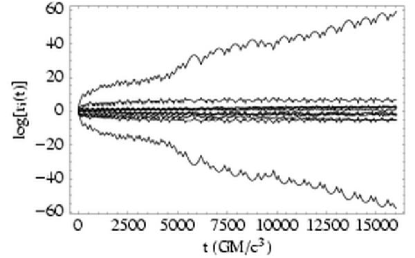
Figure 15: The natural logarithms of the ellipsoid axes $r_{i}$ vs. $t$ for the system shown in Fig. 14. Time is measured in units of $GM/c^{3}$, where $M=m_{1}+m_{2}$ is the total mass of the system. For two 10 solar-mass black holes, the time unit is $GM/c^{3}=20\,GM_{\odot}/c^{3}=10^{-4}~{}\mathrm{s}$. The spin magnitudes are fixed, so that each spin vector represents only two true degrees of freedom. We deal with this constraint by using the restricted Jacobian method (Sec. III.3). Two nonzero exponents are clearly visible, but all the others are consistent with zero. Note the $\pm\lambda$ symmetry characteristic of Hamiltonian systems.

III.4 Constrained ellipsoid method

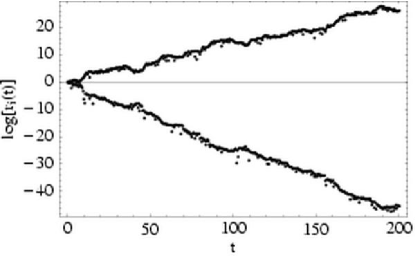
Figure 16: The natural logarithms of both ellipsoid axes $r_{i}$ vs. $t$ for the constrained forced damped pendulum, calculated using the constrained ellipsoid method (Sec. III.4). The slopes are the Lyapunov exponents. The results agree well with the unconstrained case (Fig. 9 and Table 1).

The restricted Jacobian method relies on eliminating spurious degrees of freedom from the Jacobian matrix, but such a prescription relies on making a choice—namely, which coordinates to eliminate. Each choice results in a different Jacobian matrix. Since calculating the Jacobian matrix even once can be a formidable task for sufficiently complicated systems, it is valuable to have a method that uses the full Jacobian—treating all coordinates as independent—which can be calculated once and then never touched again. This requirement leads to the constrained ellipsoid method, which uses the full Jacobian matrix to evolve constraint-satisfying tangent vectors, collectively referred to as a “constrained ellipsoid.” When recording ellipsoid axis growth, we extract from each vector a number of components equal to the true number of degrees of freedom, resulting in vectors that can be orthogonalized and (if necessary) normalized just as in the unconstrained case.

A detailed description of the constrained ellipsoid algorithm appears below, but we first present an important prerequisite: calculating constraint-satisfying tangent vectors. Let a tilde denote a vector with dimension $d$ equal to the true number of degrees of freedom (as in Sec. III.1). We construct a full tangent vector $\bm{\xi}$ (with $n$ components) from a $d$-dimensional vector $\tilde{\bm{\xi}}$ at a point $\mathbf{y}$ on the flow as follows:

1. Let $\tilde{\mathbf{y}}^{\prime}=\tilde{\mathbf{y}}+\epsilon\tilde{\bm{\xi}}$ for a suitable choice of $\epsilon$.

2. Fill in the missing components of $\tilde{\mathbf{y}}^{\prime}$ using the constraints to form $\mathbf{y}^{\prime}$ as in Sec. III.1.

3. Infer the full tangent vector $\bm{\xi}$ using

   $$\bm{\xi}=\frac{\mathbf{y}^{\prime}-\mathbf{y}}{\epsilon}.$$ (59)

Setting the initial conditions is now simple: form a random $d\times d$ matrix, orthonormalize it, and then infer the full $d\times n$ matrix using the method above on each column. The construction of constraint-satisfying tangent vectors described above is also necessary in the reorthogonalization steps of the constrained ellipsoid method.

The full method is an adaptation of the Jacobian method from Sec. II.2.4:

1. Construct a random $d\times d$ matrix and orthonormalize it to form a unit ball. Use the constraints to infer the full $d\times n$ matrix $\mathbf{U}$.

2. Evolve the system forward using the equations of motion and the evolution equation for $\mathbf{U}$,

   $$\dot{\mathbf{U}}=\mathbf{Df}\cdot\mathbf{U}.$$ (60)

3. At each time $T$, extract the relevant eight components from each tangent vector to form a $d\times d$ ellipsoid, orthonormalize it, and then fill in the missing components using the constraints, yielding again a $d\times n$ matrix. The restricted norms of the $d$ tangent vectors contribute to the running sum for the logs of the ellipsoid axes [Eq. (28)].

It is important to note that, unlike the other Jacobian methods, rescaling every time time $T$ (or some similar method) is required for the inference equation [Eq. (59)], since the product of $\epsilon$ and the components of $\bm{\xi}$ must be small for the inference to work correctly. The method only works if the system is renormalized regularly, so the value of $T$ should be chosen to be small enough that no principal ellipsoid axis grows too large.

As before, we use the constrained FDP model for purposes of illustration. Treating each coordinate as independent yields [upon differentiation of Eq. (III)]:

$$\mathbf{Df}=\left(\begin{array}[]{ccc}\frac{\partial\dot{x}}{\partial x}&\frac{\partial\dot{x}}{\partial y}&\frac{\partial\dot{x}}{\partial\omega}\\ \frac{\partial\dot{y}}{\partial x}&\frac{\partial\dot{y}}{\partial y}&\frac{\partial\dot{y}}{\partial\omega}\\ \frac{\partial\dot{\omega}}{\partial x}&\frac{\partial\dot{\omega}}{\partial y}&\frac{\partial\dot{\omega}}{\partial\omega}\\ \end{array}\right)=\left(\begin{array}[]{ccc}0&~{}-\omega{}{}&-y\\ \omega&~{}~{}0{}{}&x\\ 0&~{}-1{}{}&-c\\ \end{array}\right)$$ (61)

The coordinates are not independent, of course, but this Jacobian matrix satisfies Eq. (11) as long as the deviation is constraint-satisfying. For example, using the full deviation vector $\delta\mathbf{y}=(\delta x,\delta y,\delta\omega)$ with Eq. (61) gives the same result as the restricted deviation vector $\delta\tilde{\mathbf{y}}=(\delta x,\delta\omega)$ with Eq. (55), as long as $\delta y=-(x/y)\,\delta x$. As a result, the Lyapunov exponents calculated with the constrained ellipsoid method (Fig. 16) agree closely with the restricted Jacobian method (and with the original unconstrained results [Fig. (9)]).

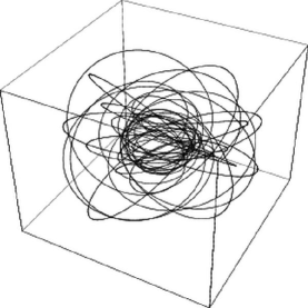
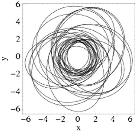
Figure 17: The orbit of a small spinning compact object (such as a solar-mass black hole) in the spacetime of a rotating supermassive black hole. (a) The orbit embedded in spherical polar coordinates; (b) the orbit’s projection onto the $x$-$y$ plane. The lengths are expressed in terms of $GM/c^{2}$, where $M$ is the mass of the central black hole. For a maximally spinning black hole, the horizon radius is $r_{H}=GM/c^{2}$. For the supermassive black hole at the center of the Milky Way, $M=3\times 10^{6}\,M_{\odot}$ Genzel et al. (2000), which corresponds to a length unit of $GM/c^{2}=4.4\times 10^{9}\,\mathrm{m}$. The system shown here is chaotic (Fig. 18), although this orbit represents a limiting case of the equations that is not physically realizable Hartl (2003a).

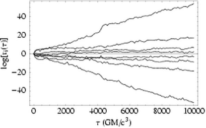
Figure 18: The natural logarithms of the ellipsoid axes for the system shown in Fig. 17 vs. relativistic proper time $\tau$, in units of $GM/c^{3}$, where $M$ is the black hole’s mass. For the supermassive black hole at the center of the Milky Way, $M=3\times 10^{6}\,M_{\odot}$ Genzel et al. (2000), which corresponds to a time unit of $GM/c^{3}=15\,\mathrm{s}$. The largest Lyapunov exponent is $\lambda_{\mathrm{max}}\approx 5\times 10^{-3}\,(GM/c^{3})^{-1}$, which corresponds to an $e$-folding timescale of $\tau_{\lambda}=1/\lambda=2\times 10^{2}\,GM/c^{3}$. For $M=3\times 10^{6}\,M_{\odot}$, this means that nearby trajectories diverge by a factor of $e$ in the local (Lorentz) frame of an observer on this orbit in a time $\tau=3000\,\mathrm{s}=50\,\mathrm{min.}$ We find nonzero exponents in this system only for physically unrealistic values of the small body’s spin (Hartl (2003b)).

As a final example of the constrained ellipsoid method, consider Fig. 17, which shows a solution to equations that model a relativistic spinning test particle (e.g., a black hole or neutron star) orbiting a supermassive rotating black hole. (The case illustrated is a limiting case of the equations, which is mathematically valid but not physically realizable; see Hartl (2003a).) These equations (usually called the Papapetrou equations) are highly constrained, so a naïve calculation of the Lyapunov exponents is not correct. It was the complicated nature of the Jacobian matrix for this system that originally motivated the development of the methods in this section Hartl (2003a). A Lyapunov plot corresponding to the orbit in Fig. 17 is shown in Fig. 18. Note especially the $\pm\lambda$ symmetry, a result of the Hamiltonian nature of the equations of motion.

IV Comparing the methods

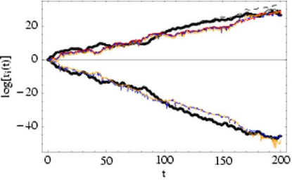
Figure 19: Natural logarithms of the ellipsoid axes vs. $t$ for the unconstrained deviation vector method (dashed), the unconstrained Jacobian method from Fig. 9 (thick) and all the constrained methods. The constrained methods include the following: rescaled deviation vector (black), Jacobian with single constraint-satisfying tangent vector (red), restricted Jacobian (orange), and constrained ellipsoid (dashed blue). (The colors appear as shades of gray in print versions of this paper.) All the constrained methods start with exactly the same initial conditions.

A summary plot of all the methods discussed in this paper, applied to the forced damped pendulum, appears in Fig. 19. It is evident that all the methods agree closely. A more quantitative comparison appears in Table 1, which gives error estimates based on integrations using fixed initial conditions and random initial deviations. This table was produced by using an initial point produced from the final values of a previous long integration, which avoids any transient effects due to starting at a point not on the attractor. The estimates for the exponents use a final time of $t_{f}=10^{4}$, with 100 randomly chosen values for the deviation vector or initial ball. All the methods agree on the mean exponents to within one standard deviation of the mean. (Recall that we omit the zero exponent associated with the time “degree of freedom.”)

Table 1: Comparison of different Lyapunov exponent methods applied to the forced damped pendulum. We consider both the unconstrained [Eq. (II.4.2)] and constrained [Eq. (III)] formulations. The integrations have a final time $t_{f}=10^{4}$, and for each method we consider 100 random initial deviations. We calculate the positive exponent ($\lambda_{1}$) and, if possible, the negative exponent ($\lambda_{3}$) as well. (We omit the zero exponent ($\lambda_{2}$) for brevity.) The error estimates are the standard deviations in the mean, $\sigma/\sqrt{N}$. The deviation vector methods are all rescaled. The constrained ellipsoid method rescales and reorthogonalizes every time $T=1$, and uses a value of $\epsilon=10^{-6}$ for the tangent-vector inference [Eq. (59)]. The error goal is a fractional error of $10^{-10}$ per step.

Method	$\lambda_{1}$	$\lambda_{3}$
unconstrained deviation vector	$0.1610\pm 0.00050$
unconstrained Jacobian	$0.1608\pm 0.00050$	$-0.2618\pm 0.00053$
constrained deviation vector	$0.1608\pm 0.00051$
constrained Jac. (1 tangent vector)	$0.1605\pm 0.00048$
restricted Jacobian	$0.1607\pm 0.00048$	$-0.2614\pm 0.00055$
constrained ellipsoid	$0.1605\pm 0.00050$	$-0.2617\pm 0.00051$

IV.1 Speed

The various methods for calculating the exponents differ significantly in their execution time, as shown in Table 2. Generally speaking, the deviation methods are faster than their Jacobian method counterparts, which is no surprise—the deviation vector methods involve fewer differential equations. More surprising is the performance penalty for the restricted Jacobian method. This is the result of a significantly smaller typical step-size in the adaptive integrator needed to achieve a particular error tolerance. The restricted Jacobian may result in a system of equations that is more difficult to integrate because of the elimination of simple degrees of freedom with the potentially complicated solutions to the constraint derivative equations $\partial{C_{k}}/\partial{y_{i}}=0$ [Eq. (57)]. On the other hand, the performance penalty of the restricted Jacobian method is probably worth the gain in robustness, as discussed below. Moreover, for other systems (e.g., the system shown in Figs. 14 and 15), the restricted Jacobian method is comparable in speed to the other Jacobian methods.

Table 2: Timing comparison for different Lyapunov exponent methods applied to the forced damped pendulum. The times (on a 2 GHz Pentium 4) for a final time of $t_{f}=10^{4}$ are in seconds: $t_{1}$ for the positive exponent $\lambda_{1}$ and $t_{1\mathrm{-}3}$ for the negative exponent $\lambda_{2}$; we omit the zero exponent ($\lambda_{2}$) for brevity. (We write $1\mathrm{-}3$ to emphasize that calculating $\lambda_{3}$ also calculates $\lambda_{1}$ as a side-effect.) We consider both the unconstrained [Eq. (II.4.2)] and constrained [Eq. (III)] formulations. The integrations use a C++ Bulirsch-Stoer integrator adapted from Press et al. (1992). The deviation vector methods are rescaled, and the constrained ellipsoid method rescales and reorthogonalizes every time $T=1$. The error goal is a fractional error of $10^{-10}$ per step. The relatively small difference between deviation vector and Jacobian methods is the result of the small number of degrees of freedom; for larger systems (with larger Jacobians) the difference can become large Hartl (2003b). We note that the restricted Jacobian method is unusually slow for the forced damped pendulum, but this is not generally the case.

Method	$t_{1}$	$t_{1\mathrm{-}3}$
unconstrained deviation vector	$2.57$
unconstrained Jacobian	$3.65$	$5.16$
constrained deviation vector	$3.51$
constrained Jacobian (1 tangent vector)	$4.05$
restricted Jacobian	$35.3$	$45.0$
constrained ellipsoid	$4.30$	$5.88$

IV.2 Robustness

Numerical methods are more useful if they are relatively insensitive to small changes in implementation details, and the Jacobian methods win in this category. When reorthogonalization occurs every time step, without rescaling, the plain Jacobian method is virtually bulletproof. The rescaling in this case can even occur only when the tangent vector norms reach very large or small values, say $\|\bm{\xi}\|\approx 10^{\pm 100}$. This robustness also applies to the restricted Jacobian method, which is considerably less finicky than any other method for constrained systems, and we recommend its implementation if practical.

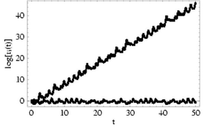
Figure 20: The natural logarithms of the two larger ellipsoid axes for the Lorenz system using the Gram-Schmidt algorithm, with the axes rescaled every $T=10^{-3}$. The largest and smallest directions differ by less than $2\%$ when rescaling this frequently, but the axes nevertheless converge rapidly to the correct directions (as determined by the Jacobian method, Fig. 6). Numerical investigations confirm that this robustness persists at least down to $T=10^{-5}$.

Jacobian methods that rescale and reorthogonalize every time $T$ are less robust, since a priori we have no knowledge of appropriate values for $T$. Experimentation in this case is required to find good values of $T$; for the Lorenz system, $T=1$ works well, but $T=5$ leads to inaccurate estimates for the negative exponent, as seen in Fig. 21. It is better to err in the direction of small times, since the Gram-Schmidt procedure is quite robust: even when rescaling occurs on very short timescales—so that the longest axis has almost no chance to outgrow the other principal axes—the Gram-Schmidt method still converges to the correct exponents (Fig. 20). Using the Gram-Schmidt algorithm to find the principal axes benefits from a strong feedback mechanism, insuring rapid convergence to the correct axes. Using a very small value for $T$ greatly increases the execution time, of course. A useful prescription in practice is to do a short integration with $T$ chosen to be small compared to any characteristic timescales in the problem, in order to obtain a first estimate for the exponents. We may then choose $T$ to be as large as we like, consistent with the avoidance of unacceptable roundoff error.

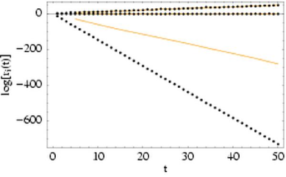
Figure 21: The natural logarithms of the ellipsoid axes for the Lorenz system, with reorthogonalization/rescaling every time $T=1$ (dark dots) and $T=5$ (light lines). The two larger exponents agree exactly, but the negative exponent is incorrect due to roundoff error, since the smallest axis shrinks from unity to a size of $e^{-5\times 14.57}\approx 2\times 10^{-32}$ in a time $T=5$.

The constrained ellipsoid method is dependent on frequent rescaling to keep the size of the tangent vectors small, since the inference scheme represented by Eq. (59) fails for large vector norms. As a result, this method suffers from the complexity of all time $T$ methods, i.e., it requires care in choosing an appropriate value of $T$. In addition, the value of $\epsilon$ in Eq. (59) must be chosen carefully to achieve accurate tangent-vector inferences: the method relies on small values of $\epsilon$ for accuracy, but values that are too small suffer from roundoff errors. It is advisable to calibrate the value of $\epsilon$ so that the largest Lyapunov exponent agrees with the result of a second method (such as the single tangent-vector method or the deviation vector method), as discussed in Hartl (2003a). Such a calibration was required to produce the values in Table 1; the largest exponent calculated using the constrained ellipsoid method differs from the other methods by several standard deviations when using $\epsilon=10^{-5}$ for the inference, but agrees well when using $\epsilon=10^{-6}$.

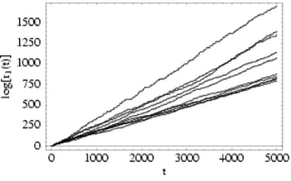
Figure 22: The natural logarithms of the largest ellipsoid axis for the constrained forced damped pendulum, calculated using the rescaled deviation vector method for varying sizes of the initial deviation. We vary the size of the initial deviation vector from $\epsilon_{0}=10^{-4}$ (bottom) to $\epsilon_{0}=10^{-13}$ (top). Values of $\epsilon_{0}$ between $10^{-4}$ and $10^{-8}$ agree closely, but smaller values lead to erroneously high values for the Lyapunov exponent. It is important to calibrate the deviation vector method using the Jacobian method (Sec. II.2) if possible.

Finally, the deviation vector methods are all very fast, but they are sensitive to the size $\epsilon_{0}$ of the initial deviation vector. The rescaled methods are particularly inaccurate if the value of $\epsilon_{0}$ is too small, which leads to roundoff error in the initial size of the deviation vector and can give inaccurate results, as shown in Fig. 22. These methods should be used with care, and should always be double-checked with a Jacobian method if possible.

V Summary and conclusion

Chaotic solutions exist for an enormous variety of nonlinear dynamical systems. Lyapunov exponents provide an important quantitative measure of this chaos. We have presented a variety of different methods for calculating these exponents numerically, both for constrained and unconstrained systems. Both types of systems can be investigated using deviation vector methods or Jacobian methods. Deviation vector methods use the equations of motion to evolve two nearby trajectories in phase space to determine the time-evolution of the small deviation vector joining the trajectories. This family of methods is computationally fast, but yields only the largest exponents, and also suffers from sensitivity to the size of the initial deviations. The Jacobian methods share the use of the Jacobian matrix of the system as a rigorous measure of the local phase-space behavior. They are computationally robust in general, and can be used to determine multiple exponents, but this comes at the cost of execution speed.

Calculating Lyapunov exponents for constrained systems presents a variety of complications, all revolving around the notion of constraint-satisfying deviations: “nearby” trajectories must be chosen carefully to insure that they satisfy the constraints. We have presented several methods for dealing with these complications, including a deviation vector method and two Jacobian methods: the restricted Jacobian method, which eliminates spurious degrees of freedom in the Jacobian by differentiating the constraints; and the constrained ellipsoid method, which uses the full Jacobian matrix to evolve constraint-satisfying tangent vectors. These methods allow the determination of all $d$ Lyapunov exponents for systems with $d$ degrees of freedom.

Appendix A Ellipsoid axes and the singular value decomposition

In this appendix, we discuss an alternative method for calculating the ellipsoid axes used in the Jacobian method, namely, calculating the ellipsoid axes exactly. The method described seems superior on paper to the Gram-Schmidt technique described in Sec. II.2, but suffers from subtle complications that make it fragile in practice. Nevertheless, within a narrow range of validity (specified below), calculating exact ellipsoid axes provides valuable corroboration of the principal Jacobian method discussed above.

Recall Theorem 1 from Sec. II.2.3, which relates the eigensystem of the matrix $A^{T}A$ to the ellipsoid spanned by the columns of $A$. In order to find the axes of an evolving ellipsoid, we could apply Theorem 1 directly, but there is a mathematically equivalent prescription that is numerically virtually bulletproof, namely, the famous singular value decomposition:

Theorem 2

Let $A$ be a nonsingular $n\times n$ matrix. Then there exist orthonormal $n\times n$ matrices $U$ and $V$, and a diagonal matrix $S$, such that

$$A=USV^{T}.$$ (62)

This is the singular value decomposition (SVD) of $A$, and the values $s_{i}$ in $S=\mathrm{diag}(s_{1},\ldots,s_{n})$ are the singular values.

Since $V$ is an orthogonal matrix, we have $V^{T}=V^{-1}$, so that Eq. (62) is equivalent to $AV=US$. Geometrically, this means that the image of the unit ball $V$ is equal to an ellipsoid whose $i$th principal axis is given by $s_{i}$ times the $i$th column of $U$. $V$ in this context is a special ball, but the image of any unit ball is the same unique ellipsoid. This leads to the following theorem:

Theorem 3

Let $A$ be a nonsingular $n\times n$ matrix, and let $U$ and $S$ be the matrices resulting from the singular value decomposition of $A$ [Eq. (62)]. Then the columns of $A$ span an ellipsoid whose $i$th principal axis is $s_{i}\,\mathbf{u}_{i}$, where $S=\mathrm{diag}(s_{1},\ldots,s_{n})$ and $\{\mathbf{u}_{i}\}_{i=1}^{n}$ are the columns of $U$.

We thus see that the singular value decomposition is equivalent to finding the eigensystem of $A^{T}A$. (See Appendix A in Alligood et al. (1997) for proofs of these theorems.)

Figure 23: The natural logarithms of the two larger ellipsoid axes for the Lorenz system using the singular value decomposition. The axes are rescaled every $T=0.5$ to exaggerate the deviations from the correct results, but any rescaling causes the SVD method to fail (see text). Compare to unrescaled SVD (Fig. 24) and the Gram-Schmidt method with frequent rescaling (Fig. 20).

Substituting the singular value decomposition for the Gram-Schmidt procedure leads to a replacement of step (2) from Sec. II.2:

• At various times $t_{j}$, replace $\mathbf{U}$ with the orthogonal axes of the ellipsoid defined by $\mathbf{U}$, using the singular value decomposition. This can be done either every time $T$, for some suitable choice of $T$, or every time the integrator takes a step. It is essential to order the principal axes consistently. We recommend sorting the axes so that $s_{1}\geq s_{2}\geq\ldots\geq s_{n}$.

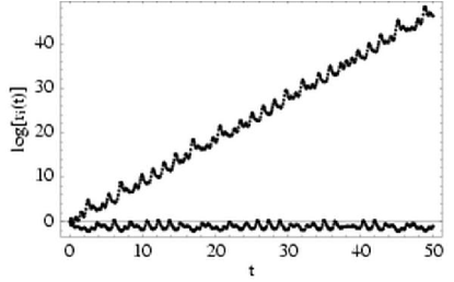
Figure 24: The natural logarithms of the two larger ellipsoid axes for the Lorenz system using the singular value decomposition, without rescaling. The results agree well with the Gram-Schmidt method (Fig. 6). Rescaling (which is always necessary if we approach the floating point limits of $\sim\!\!10^{\pm 308}$) ruins the agreement.

Unfortunately, this prescription behaves badly when rescaling is necessary, as shown in Fig. 23. The underlying cause of this is a fundamental property of the singular value decomposition: it is only unique up to a permutation of the ellipsoid axes. If we adopt an ordering based on the axis lengths, we can refer, for example, to the longest axis as axis 1. During any particular time period, axis 1 may grow or shrink; the only requirement is that it be the fast-growing axis on average. Unfortunately, rescaling the axes causes this ordering method to fail: if axis 1 should happen to contract between rescaling times, then the ordering based on length leads to incorrect axis labels, since axis 1 is no longer the longest axis. Even worse, when ordering by axis length, the length of the longest axis is always added to the running sum for the largest Lyapunov exponent, while the length of the smallest axis always contributes to the smallest exponent. This selection bias leads to systematic errors, guaranteeing overestimates for the absolutes values of both the exponents (Fig. 23).

If the system is not rescaled, there is still some initial ambiguity in axis labels, but once axis 1 has grown sufficiently large it is very unlikely ever to become smaller than the other axes. Thus, after an initial expansion and contraction phase that establishes the ordering, the axis labels remain fixed, and the results of the (unrescaled) SVD method agree well with Gram-Schmidt (Fig. 24).

It should be possible in principle to follow the axis evolution by tracking the continuous deformation of the ellipsoid. This would mean assigning labels to the axes and then ensuring, e.g., that axis 1 at a later time is indeed the image of the original axis 1. This method would require following the system over very short timescales to guarantee the correct tracking of axes, and even then is likely to be fragile and error-prone. Because of these complications, we recommend the simpler Gram-Schmidt process, which has proven to be reliable and robust in practice.

References

- Lorenz (1963) E. Lorenz, J. Atmospheric Science 20, 130 (1963).
- Colonna and Bonasera (1999) M. Colonna and A. Bonasera, Phys. Rev. E 60, 444 (1999).
- Yamaguchi and Iwai (2001) Y. Y. Yamaguchi and T. Iwai, Phys. Rev. E 64, 066206 (2001).
- (4) G. A. Gottwald and I. Melbourne, eprint nlin.CD/0208033.
- Ryabov (2002) V. B. Ryabov, Phys. Rev. E 66, 016214 (2002).
- Vallejos and Anteneodo (2002) R. O. Vallejos and C. Anteneodo, Phys. Rev. E 66, 021110 (2002).
- (7) J. D. Barrow and J. Levin, eprint nlin.CD/0303070.
- Alligood et al. (1997) K. T. Alligood, T. D. Sauer, and J. A. Yorke, Chaos: An Introduction to Dynamical Systems (Springer, New York, 1997).
- Ott (1993) E. Ott, Chaos in Dynamical Systems (Cambridge University Press, Cambridge, England, 1993).
- Hartl (2003a) M. D. Hartl, Phys. Rev. D 67, 024005 (2003a), eprint gr-qc/0210042.
- Hartl (2003b) M. D. Hartl (2003b), accepted for publication in Phys. Rev. D, eprint gr-qc/0302103.
- (12) M. D. Hartl, http://www.michaelhartl.com/software/.
- Eckmann and Ruelle (1985) J.-P. Eckmann and D. Ruelle, Rev. Mod. Phys. 57, 617 (1985).
- Press et al. (1992) W. H. Press, S. A. Teukolsky, W. T. Vetterling, and B. P. Flannery, Numerical Recipes in C (Cambridge University Press, Cambridge, England, 1992).
- Benettin et al. (1980) G. Benettin, L. Galgani, A. Giorgilli, and J.-M. Strelcyn, Meccanica 15, 21 (1980).
- Damour (2001) T. Damour, Phys. Rev. D 64, 124013 (2001).
- Damour et al. (2000) T. Damour, P. Jaranowski, and G. Schäfer, Phys. Rev. D 62, 084011 (2000).
- Damour and Schäfer (1988) T. Damour and G. Schäfer, Nuov. Cimento 101, 127 (1988).
- Genzel et al. (2000) R. Genzel, C. Pichon, A. Eckart, O. E. Gerhard, and T. Ott, Mon. Not. Royal Astron. Soc. 317, 348 (2000).