Are Aftershocks of Large Californian Earthquakes Diffusing?

Abstract

We analyze 21 aftershock sequences of California to test for evidence of space-time diffusion. Aftershock diffusion may result from stress diffusion and is also predicted by any mechanism of stress weakening. Here, we test an alternative mechanism to explain aftershock diffusion, based on multiple cascades of triggering. In order to characterize aftershock diffusion, we develop two methods, one based on a suitable time and space windowing, the other using a wavelet transform adapted to the removal of background seismicity. Both methods confirm that diffusion of seismic activity is very weak, much weaker than reported in previous studies. A possible mechanism explaining the weakness of observed diffusion is the effect of geometry, including the localization of aftershocks on a fractal fault network and the impact of extended rupture lengths which control the typical distances of interaction between earthquakes.

HELMSTETTER et al. Diffusion of Aftershocks 2003JB***** Agnès Helmstetter, Institute of Geophysics and Planetary Physics, University of California, Los Angeles, California. (e-mail: helmstet@moho.ess.ucla.edu) Guy Ouillon, Laboratoire de Physique de la Matière Condensée, CNRS UMR 6622 Université de Nice-Sophia Antipolis, Parc Valrose, 06108 Nice, France (e-mail: Ouillon@aol.com). Didier Sornette, Laboratoire de Physique de la Matière Condensée, CNRS UMR 6622 Université de Nice-Sophia Antipolis, Parc Valrose,06108 Nice, France, and Department of Earth and Space Sciences and Institute of Geophysics and Planetary Physics, University of California, Los Angeles, California. (e-mail: sornette@naxos.unice.fr)

¹ Institute of Geophysics and Planetary Physics, University of California, Los Angeles, California 90095 ² Laboratoire de Physique de la Matière Condensée, CNRS UMR6622 and Université des Sciences, Parc Valrose, 06108 Nice Cedex 2, France. ³ Department of Earth and Space Sciences, University of California, Los Angeles, California 90095

1 Introduction

Aftershocks are defined by their clustering properties both in time and space. The temporal clustering obeys the well established (modified) Omori law [Utsu et al., 1995] which states that the rate of aftershocks decays as

$$n(t)=\frac{A}{(t+c)^{p}}~{},$$ (1)

where the Omori exponent $p$ is generally found between $0.5$ and $2$. In expression (1), the origin of time is the occurrence of the main event. The offset time $c$ is often not well-constrained and may partly account for the incompleteness of catalogs close to mainshocks. It provides a regularization at short times preventing the event rate to reach infinity at the time of the mainshock. This law with the cut-off $c$ may be derived from a variety of physical mechanism (e.g. [Dieterich, 1994]).

The spatial organization of aftershocks is more complex and less understood. On the one-hand, it is recognized that many aftershocks occur right on the fault plane or in its immediate vicinity (at the scale of the mainshock rupture length) and this is used for 3D visualization of the rupture surface (see for instance Fukuyama [1991]). The observation that the spatial distribution of earthquakes in California is characterized by a fractal dimension close to $2.2$ [Kagan and Knopoff, 1980] and the fact that this measure is dominated by aftershock clustering suggests a rather complex network of active faults [Sornette, 1991]. The clustering of aftershocks on or close to the mainshock rupture probably reflects local stress concentration at asperities that served to stop the rupture and lock the fault. On the other hand, aftershocks also occur away from fault ruptures, due to various triggering mechanism, the simplest one being stress transfer and increasing Coulomb stress [King et al., 1994; Stein et al., 1994; Stein, 1999; Toda et al., 2002].

Both temporal and spatial properties argue for the presence of triggering processes, which could also be expected to lead to combined space and time dependence of the organization of aftershocks. Indeed, several studies have reported so-called “aftershock diffusion,” the phenomenon of expansion or migration of aftershock zone with time [Mogi, 1968; Imoto, 1981; Chatelain et al., 1983; Tajima and Kanamori, 1985a,b; Ouchi and Uekawa, 1986; Wesson, 1987; Rydelek and Sacks, 1990; Noir et al., 1997; Jacques et al., 1999]. Immediately after the mainshock occurrence, most aftershocks are located close to the rupture plane of the mainshock, then aftershocks may in some cases migrate away from the mainshock, at velocity ranging from $1$ km/h to $1$ km/year [Jacques et al., 1999; Rydelek and Sacks, 2001]. This expansion is not universally observed, but is more important in some areas than in others [Tajima and Kanamori, 1985a]. Most of these studies are qualitative and are based on a few sequences at most. Marsan et al. [1999, 2000] and Marsan and Bean [2003] have developed what is to our knowledge the first systematic method to analyze space-time interactions between pairs of earthquake and report evidence for strong diffusion (see our discussion below on these results). A similar method has also been used by Huc and Main [2003]. The present state of knowledge on aftershock diffusion is confusing because contradictory results have been obtained, some showing almost systematic diffusion whatever the tectonic setting and in many areas in the world, while others do not find evidences for aftershock diffusion [Shaw, 1993]. This may reflect the intrinsic variability in space and time of genuine diffusion properties and also possible biases of the analyses, for example, due to background seismicity.

From a physical viewpoint, the diffusion of aftershocks is usually interpreted as a diffusion of the stress induced by the mainshock, either by a viscous relaxation process [Rydelek and Sacks, 2001], or due to fluid transfer in the crust [Nur and Booker, 1972; Hudnut et al., 1989; Noir et al., 1997]. However, such a stress diffusion process is not necessary to explain aftershock diffusion. Recent studies have indeed suggested that aftershock diffusion may result from either a rate and state friction model [Dieterich, 1994; Marsan et al., 2000] or a sub-critical growth mechanism [Huc and Main, 2003], without invoking any process of stress diffusion. Actually, aftershock diffusion is predicted by any model that assumes that (i) the time to failure increases if the applied stress decreases and (ii) the stress change induced by the mainshock decreases with the distance from the mainshock. Therefore, aftershocks further away from the mainshock will occur later than those closer to the mainshock, because the stress change is smaller and thus the failure time is larger. An increase of time to failure with the applied stress is predicted by many models of aftershocks, including rate and state friction [Dieterich, 1994], sub-critical crack growth [Das and Scholz, 1981; Yamashita and Knopoff, 1987; Shaw, 1993], damage or static fatigue laws [Scholz, 1968; Lee and Sornette, 2000]. For instance, the sub-critical growth model of [Das and Scholz, 1981] predicts that the time to failure $t_{c}$ of an aftershock decreases with the stress change $d\sigma$ according to

$$t_{c}\sim d\sigma^{-n}~{},$$ (2)

where $n$ is the stress corrosion index. If the stress change decreases with the distance $r$ from the mainshock according to

$$d\sigma(r)\sim r^{-1/2}$$ (3)

in the near field (at distances from the fault smaller than the mainshock rupture length), then the average time to failure increases with $r$ as

$$t_{c}(r)\sim r^{n/2}$$ (4)

By inverting $r$ as a function of $t$, the typical distance $R(t)$ of aftershocks occurring at time $t$ after the mainshock is thus expected to increase according to [Huc and Main, 2003]

$$R(t)\sim t^{H}~{},$$ (5)

with $H=2/n$. Expression (5) thus predicts a very slow sub-diffusion, with a diffusion exponent $H=2/n\approx 0.06$ for a corrosion index close to 30 as generally observed [Huc and Main, 2003]. The diffusion exponent is even smaller at large distances from the mainshock because the stress decreases as $\sim 1/r^{3}$ and thus $H=1/(3n)$. If the time to failure decreases exponentially with the applied stress, as expected for example for static fatigue laws [Scholz, 1968], the typical distance $R$ increases logarithmically with time. Such a slow diffusion is difficult to observe in real data due to the limited number of events and the presence of background seismicity. Take $H=0.2$ for instance: one needs five decades in time range to observe one decades in space range. The smallness of the diffusion exponent $H$ predicted by this and other models (see Appendix A) explains why it may be difficult to observe it.

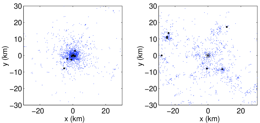
Figure 1: Maps of seismicity generated by the ETAS model with parameters $b=1$, $\theta=0.2$, $\mu=1$, $d=1$ km, $\alpha=0.5$, $c=0.001$ day and a branching ratio $n=1$. The mainshock occurs at the origin of space with magnitude $M=7$ (black star). The minimum magnitude is fixed at $m_{0}=0$. The distances between mainshock and aftershocks follow a power-law with parameter $\mu=1$ and the local Omori law is $\propto 1/t^{1+\theta}$. According to the theory developed in the text, the average distance between the first mainshock and the aftershocks is thus expected to grow as $R\sim t^{\theta/\mu}\sim t^{0.2}$. The two plots are for different time periods of the same numerical simulation, such that the same number of earthquakes $N=3000$ is obtained for each graph: (a) time between $0$ and $0.3$ days; (b) time between $30$ and $70$ yrs. At early times, aftershocks are localized close to the mainshock, and then diffuse and cluster around the largest aftershocks.

Another alternative explanation of aftershock diffusion, that does not rely on any stress diffusion process, is multiple triggering. Ouchi and Uekawa [1986] first reported that the diffusion of aftershocks is often due to the occurrence of large aftershocks and the ensuing localization of secondary aftershocks close to them. The apparent diffusion of the seismicity may thus result from a cascade process; the mainshock triggers aftershocks which in turn trigger their own aftershocks, and so on, thus leading to an expansion of the aftershock zone. A recent series of papers have investigated quantitatively this concept of triggered seismicity [Helmstetter and Sornette, 2002a,b,c; 2003a; Helmstetter et al., 2003] in the context of the so-called epidemic-type aftershock (ETAS) model of earthquakes seen as point-wise events, which was introduced by Ogata [1988] and in a slightly different form by Kagan and Knopoff [1981; 1987]. The ETAS model assumes that each earthquake triggers aftershocks, with a rate that decays in time according to Omori’s law, and which increases with the mainshock magnitude. The distribution of distances between triggered and triggering earthquake is assumed to be independent of the time. Using this model, Helmstetter and Sornette [2002b] showed that, under the right conditions (see Appendix A), the characteristic size $R$ of the aftershock cloud may increase as a function of time $t$ since the mainshock according to expression (5), where $H$ is a function of both the exponent of Omori’s law and of the exponent describing the spatial interactions between events (see Appendix A). Figure 1 presents results from numerical simulations of the ETAS model to show how cascades of multiple triggering can produce aftershock diffusion. The analysis of the ETAS model in [Helmstetter and Sornette, 2002b] offers some predictions that can be tested in real aftershock sequences. Diffusion should be observed only if the Omori exponent $p$ is smaller than 1, and the diffusion exponent $H$ should decrease with $p$ if $p<1$. In addition to the diffusion law (5), the ETAS model also predicts a decrease of the Omori exponent $p$ with the distance from the mainshock.

The fundamental difference between the diffusion predicted by the ETAS model and by models based on stress weakening mechanisms is that, in the later, diffusion derives from the direct effect of the mainshock while, in the former, there is no diffusion of direct (first generation) aftershocks and diffusion results from the cascade of secondary aftershocks.

Motivated by these different empirical and theoretical works, we revisit the issue of the existence of aftershock diffusion and of its characterization. For this, we develop two different and complementary methods to test these predictions. We analyze aftershock sequences in California and interpret the results in the lights of the predictions obtained from the ETAS model [Helmstetter and Sornette, 2002b] (see Appendix A for a brief description of the relevant predictions).

The organization of the article is as follows. We first discuss the problems encountered in previously published analyses of diffusion in real data. We then explain and use a direct method of analysis of several aftershock sequences in California, followed by a second method based on wavelet analysis. This second method aims at optimizing the removal of the perturbing influence of the seismicity background. We then discuss the limits of the theoretical and numerical analysis, and interpret our empirical results in the light of various available models.

Our analyses are carried out on two different catalogs, (i) the catalog of Southern California seismicity provided by the Southern California Seismic Network for the period 1932-2000, and (ii) the catalog of Northern California seismicity provided by the Northern California Seismic Network since 1968. The minimum magnitude for completeness ranges from $M=3.5$ in 1932 to $M<2$ for the two catalogs since 1980. The average uncertainty on earthquake location is about $1$ km for epicenters, but is larger for hypocenters. Therefore we consider only the spatial distribution of epicenters.

2 Methodological Issues

A priori, the observed seismicity results from a complex interplay between tectonic driving, fault interactions, different spatio-temporal field organizations (stress, fluid, plastic deformation, phase transformations, etc.) and physical processes of damage and rupture. Notwithstanding this complexity, from the viewpoint of empirical observations, one may distinguish two classes of seismicity: the seismicity resulting from the tectonic loading which is often taken as a constant source (uncorrelated seismicity) and the triggered seismicity resulting from earthquake interactions (correlated seismicity). An alternative classification of seismicity defines earthquakes as either foreshock, mainshock, aftershock or background seismicity. The definition of aftershocks and foreshocks requires the specification of a space-time window used to select foreshocks (resp. aftershocks) before (resp. after) a larger event defined as the mainshock. The background is the average level of seismicity prior to the mainshock or at large times after the mainshock. Of course, such classification is open to criticism in view of the inescapable residual arbitrariness of the selection of foreshocks, mainshocks and aftershocks [Helmstetter et al., 2003; Helmstetter and Sornette, 2003]. Nevertheless, it offers a useful reference for testing what is measured in earthquake diffusion processes.

Following previous studies, our analyses presented below assume that earthquake occurrence follows a point process, because we deal with the space and time organization of aftershock epicenters. Physically, this would be justified when all spatial and temporal scales are larger than source rupture dimension and duration. In reality, this is not the case and the point process representation may lead to incomplete or misleading conclusions, as we point out in section 6.3.

2.1 Effect of uncorrelated seismicity

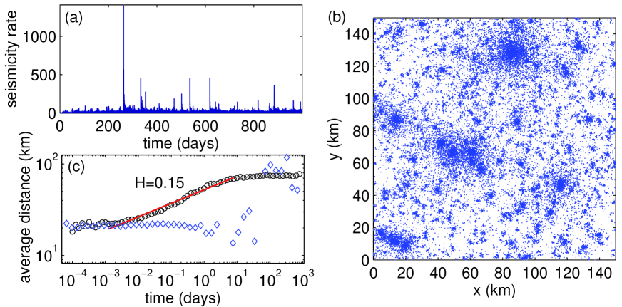
Figure 2: Analysis of a synthetic aftershock sequence. We have built a synthetic catalog by superposing a large number of independent aftershock sequences. We have used 1000 mainshocks, with a Poissonian distribution in time and space. Each mainshock generates only direct aftershocks with a rate given by (16), with $K=10$, $\alpha=0.8$, $\theta=-0.1$, $c=0.001$ day, $\mu=2$ and $d$ equal to the rupture length of the mainshock. The distribution of distances between aftershocks and mainshocks is thus independent of the time between mainshock and aftershocks. The global number of events in the catalog is 40000 including the 1000 mainshocks. The seismicity rate (a) displays several peaks corresponding to the occurrence of large mainshocks, as observed for California seismicity. The map (b) shows large clusters corresponding to the aftershock sequences of the largest mainshocks. The average distance between all pairs of events (c) shown as circles increases with the average time between events as $R\sim t^{H}$ with $H=0.15$ (solid line), for a large interval of the time between events $[0.001-10]$ days. For larger times, the average distance saturates to $R\approx 80$ km, half the size of the catalog. The diamonds show the results obtained with the method of Marsan et al. [2000]. At early times ($t<1$ day), the average distance is constant and the method is effective to remove the influence of uncorrelated seismicity. But at large times when the aftershock activity is small, there are large fluctuations of the average distance, because the method is very sensitive to the noise.

The major problem when analyzing real seismicity data in search of some evidence for diffusion comes from the mixture of correlated seismicity which can display diffusion and of uncorrelated seismicity (noise). The latter can significantly alter the evaluation of the characteristic distance of the aftershock zone. To illustrate this problem, we analyze in Figure 2 a synthetic catalog generated by superposing a large number of independent aftershock sequences, without adding a constant seismicity background. This synthetic catalog has been generated by superposing 1000 mainshocks with a Poissonian distribution in time and space and with a Gutenberg-Richter distribution of magnitudes, and by adding aftershocks sequences of each mainshock, with a number of aftershock increasing as $10^{0.8M}$ with the mainshock magnitude $M$. If we study, as in previous studies, the average distance between all pairs of events in the catalog as a function of their average time difference, the superposition of uncorrelated aftershock sequences induces an apparent and spurious diffusion, over almost four orders of magnitude in time. This apparent diffusion comes from the superposition of a large number of aftershock sequences, with a power-law distribution of duration and spatial extension, resulting from the increase of the number of aftershocks and of the length of the aftershock zone with the mainshock magnitude, together with a power-law distribution of earthquakes sizes (Gutenberg-Richter law).

In order to study the diffusion of aftershocks, triggered directly or indirectly by the same source, one strategy is to study individual aftershock sequences of large earthquakes selected by some clustering algorithm, in order to remove the influence of uncorrelated seismicity. This is the approach followed in the present paper.

2.2 Discussion of the method of Marsan et al.

In contrast, Marsan et al. [Marsan et al., 1999; 2000; Marsan and Bean, 2003] have proposed a different method, which uses all available seismicity and considers all pairs of events independently of their magnitude, with the advantage that (1) the corresponding data set is much larger than for individual aftershock sequences and (2) their method does not require the sometimes arbitrary definition of mainshocks and aftershocks. In principle, their approach provides a systematic search of possible space-time correlations between earthquakes. However, there is a potential problem with their method stemming from the effect of the background seismicity and of uncorrelated seismicity, as illustrated in figure 2. Indeed, they study the average distance between all points as a function of the time between them. Therefore, their count is performed over a mixture of very different earthquake populations, a significant fraction of events being probably unrelated causally.

In order to remove the influence of this uncorrelated seismicity, they use the global catalog to estimate the average distance between two points, and they remove the contribution of the average seismicity to estimate the spatio-temporal distribution of the correlated seismicity. Specifically, Marsan et al. calculate a pair-wise time-dependent space-space correlation function corrected for the background by subtracting the long-time average value of this space-space correlation function, from which they estimate an average distance between pairs as a function of time. The growth of this average distance with time may then qualify a causal dependence between earthquakes, through a diffusive process. Marsan and others [Marsan et al., 1999; 2000; Marsan and Bean, 2003] studied in this way several catalogs at different spatial scales, from the scale of a mine to world-wide seismicity, and observed that the average distance between two earthquakes increases as a power-law of the time between them, with an exponent often close to $H=0.2$, indicative of a sub-diffusion process. They interpreted their results as a mechanism of stress diffusion, that may be due to fluid transfer with heterogeneous permeability leading to sub-diffusion.

In this sense, Marsan et al. do not try to establish a causal dependence between earthquakes but rather to detect a correlation in their spatio-temporal organization. Recall that correlation shows that two events are related, but it does not determine their cause and effect relationship. This is because there are basically three possible explanations for the observation of correlation: (i) The correlation is a coincidence; (ii) One event causes the other; (iii) The two events are both caused by some third event. In their detection of spatio-temporal correlations in seismicity, Marsan et al. do not distinguish between explanation (ii) nor (iii) while in contrast the present paper emphasizes explanation (ii).

We have performed many tests of Marsan et al.’s method on synthetic catalogs. A typical test is shown as the diamond symbols in figure 2. At early times ($t<1$ day), the average distance between earthquake pairs is constant, as it should be, and the method removes adequately the influence of uncorrelated seismicity. But at large times when aftershock activity is small, the average distance exhibits large fluctuations as a function of time. This is due to the corrective term which becomes ill-conditioned at large times and leads to a large sensitivity to noise and finite sample sizes. We have found that, in most of our synthetic catalogs constructed without genuine diffusion, the average distance obtained by Marsan et al.’s method is approximately constant at early times as it should, but then crosses over to another noisy plateau at long times, as a result of the ill-defined correction term. This noisy crossover from a constant to another higher plateau obviously gives an apparent growth of the average distance between pairs of earthquakes as a function of time, which may compete with or hide a genuine signal. It seems to us that several of the figures on the time dependence of the average distance, which are presented in [Marsan et al., 1999; 2000; Marsan and Bean, 2003], exhibit this feature of a more or less constant or very weak growth followed by a more abrupt jump to another noisy plateau. If one interprets Marsan et al.’s results in terms a causal diffusion processes, the evidence on diffusion provided in [Marsan et al., 1999; 2000; Marsan and Bean, 2003] is only suggestive and additional tests of the methods on synthetic and real data should be performed in order to understand its effects on the analysis of real data and to improve the correction term. Marsan et al.’s analysis is perhaps better interpreted as evidence of a spatio-temporal correlation of seismicity resulting from viscous relaxation, stress pulses and other processes operating at large scales. But then, their analyses should not be interpreted using models of causal diffusion based on rate- and state-dependent friction law [Marsan et al., 2000] or on sub-critical crack growth [Huc and Main, 2003], that model only mainshock-aftershock pairs and not arbitrary pairs of earthquakes.

3 Windowing method

3.1 Method

In this study, we analyze individual aftershock sequences and consider the diffusion of the seismicity triggered directly or indirectly by the mainshock. We adjust the values of the time window $T$ and the space window $D$ used to select aftershocks so that the rate of background activity is negligible in comparison with the aftershock rate. The background seismicity rate is estimated by the average seismicity before the mainshock. We also adjust the minimum magnitude $m_{0}$ and the minimum time $t_{min}$ after the mainshock in order to obtain a catalog that is complete for $t_{min}<t<T$ and $m>m_{0}$.

In order to estimate the average size $R$ of the aftershock area as a function of the time from the mainshock, we define the barycenter of the aftershock sequence as the reference point because the mainshock epicenter has no reason a priori to be the source of the aftershock sequence. The average size of the aftershock area $R$ is obtained as the average distance between the aftershocks and the barycenter. We find that this procedure yields a diffusion exponent $H_{r}$ that is always a little larger than the diffusion exponent estimated from the average distance between the aftershocks and the mainshock epicenter, as done in Marsan et al. [1999; 2000], Marsan and Bean [2003] and Huc and Main [2003]. We also introduce a refinement to take into account the anisotropy of the aftershock zone and the spatial extension of the mainshock rupture. For this, we compute the axes $a$ and $b$ of inertia of the whole aftershock sequence as a function of the time after the mainshock, in the spirit of Kagan [2002]. Geometrically, this corresponds to approximating the map of aftershocks as filling an ellipse with small axis $b$ and large axis $a$. This provides two additional diffusion exponents $H_{a}$ and $H_{b}$. For strike-slip mainshocks, $b(t)$ measures the average distance between aftershocks and the fault plane, while the large axis gives the average distance between aftershocks and the barycenter on the fault plane.

We also measure the Omori exponent by plotting the rate of aftershock activity as a function of time in a log-log plot, and by measuring the slope $p$ by a linear regression for $t_{min}<t<T$. We have also used a maximum likelihood method to estimate both the $p$ and $c$ values of the modified Omori law. In most cases, the two methods provide similar values of $p$. We also estimate the variation of $p$ with the distance $r$ between the mainshock and its aftershocks by selecting aftershocks at different distances between the mainshock. As described in Appendix A, a prediction of the ETAS model concerns the modification of the distribution of distances $r$ between aftershocks and the mainshock epicenter with time. We plot the distribution of distances $r$ between the mainshock and its aftershocks for several time windows to test if there is an expansion of the aftershock area with time.

We have tested this method using synthetic catalogs generated with the ETAS model, including a constant seismicity background. We have checked that our method provides a reliable estimate of the diffusion exponent and is almost insensitive to the background activity as long as the duration of the time window is sufficiently short so that the seismicity is dominated by aftershocks.

3.2 Results

We have analyzed 21 aftershock sequences of major earthquakes in California with number of aftershocks larger than 500, in addition to two aftershock sequences of large earthquakes (Kern-County, M=7.5, 1952, and San-Fernando, M=6.6, 1971) which have less than 500 events. The results for all these 21 sequences are listed in Table LABEL:tabdifobs. The different values of $H$, measured either by the average distance from the barycenter ($H_{r}$) or from the inertial axes ($H_{a}$ and $H_{b}$), generally give similar results. Exceptions are the Morgan Hill, Loma-Prieta, and Joshua-Tree events which have $H_{b}>H_{a}$, and the Imperial Valley event which gives $H_{b}<H_{a}$. The diffusion exponent $H$ is always positive, and generally smaller than $0.1$. The estimated standard deviation on $H$, measured for synthetic catalogs with the same number of events and similar $p$-values, is about 0.05. Thus, most aftershock sequences do not exhibit significant diffusion.

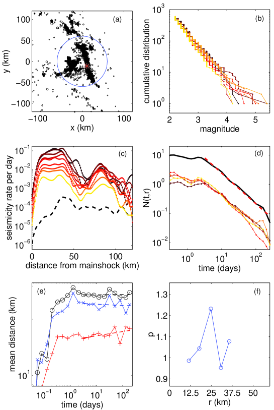
Figure 3: Analysis of the June, 28, 1992, $M=7.3$ Landers aftershock sequence. (a) Map of aftershocks, the mainshock epicenter is shown by a star. (b) Magnitude distribution for different time windows (time increasing from black to gray) showing that the magnitude distribution is stable over time, and that the catalog is complete above $m=2.2$ after 3 days after the mainshock. (c) Rate of seismic activity as a function of the distance from the mainshock for different times after the mainshock (increasing time from top to bottom (black to gray)). The background activity preceding the mainshock is shown as a dashed line. (d) Rate of aftershocks for the whole sequence (solid black line at the top) and fit by an Omori law (dashed gray line), and rate of aftershocks for different distances from the mainshock (increasing distance from gray to black). (e) Characteristic size of the aftershock cluster as a function of the time from the mainshock, measured by the average distance from the barycenter (circles), or from the small (’+’) and large (’x’) inertial axes. (f) Variation of the Omori exponent with the distance from the mainshock.

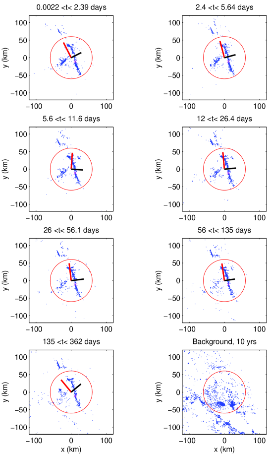
Figure 4: Map of the aftershocks of the Landers earthquake, for different time windows with 1000 events in each plot, showing the stationarity of the spatial distribution of aftershocks. The epicenter is shown by a cross. The gray and black lines show the large and small elliptical axes respectively (multiplied by a factor 2 for clarity).

Details of the analysis for the aftershock sequence following the 1992 $M=7.3$ Landers event are shown in Figures 3 and 4. For this sequence, we measure an Omori exponent $p=1.1$, which is stable when looking at different distances $r$. The characteristic cluster size is also stable over more than two orders of magnitude in time leading to $H\approx 0$. Similar results are obtained for the elliptical axes $a$ and $b$. The analysis of the distance distribution at different times also confirms that there is no discernible diffusion of seismic activity.

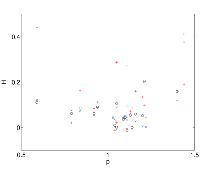
Figure 5: Diffusion exponents $H$ as a function of the Omori exponent $p$ for the aftershock sequences described in Table LABEL:tabdifobs. The circles give the diffusion exponent $H_{r}$ evaluated with the mean distance from the barycenter (radius of gyration), the crosses correspond to the diffusion exponent $H_{a}$ and the ’+’ correspond to $H_{b}$.

Figure 5 summarizes the results for $p$ and $H$ listed in Table LABEL:tabdifobs. The first result we should stress is that all our values of the diffusion exponent $H$ are quite small when compared with previous studies [Marsan et al., 1999; 2000; Marsan and Bean, 2003]. For the reasons explained in section 2, we believe that Marsan et al.’s results may have been affected by the background seismic activity, and are quantifying different processes. One can observe a weak negative correlation between $p$ and $H$ for $p<1$ but this negative correlation disappears when including data with $p>1$ which gives a very strong scatter with two among the largest $H$ obtained for the largest $p>1$.

4 Wavelet method

The detection of aftershock diffusion may be biased (i) by other (possibly) independent aftershock sequences and (ii) by background seismicity. In the windowing method, we have addressed these problems by analyzing (a) individual aftershock sequences of large earthquakes over a space-time window (b) with seismicity rate much larger than the background estimated over a ten-year average.

We now present a second method based on wavelet analysis, which introduces two innovations. First, it uses a smoothing kernel (or mother wavelet) constructed in order to remove Poissonian background seismicity. Second, it uses the expected scaling relationship relating space and time that characterizes diffusion to derive scaling laws obeyed by the wavelet coefficients. The exponents $p$ of the observed Omori law and $H$ of aftershock diffusion are then obtained by optimizing the compliance of the wavelet coefficients to these scaling laws. The wavelet approach displays the data all at once in the space and time-scale dimensions in order to determine $p$ and $H$ simultaneously. In contrast, the windowing method displays the data twice, once in the time dimension to obtain the exponent $p$ and a second time to obtain $R(t)$ and the exponent $H$. The wavelet method can thus be seen as a simultaneous two-dimensional time scale-space determination of $p$ and $H$, in contrast with the previous windowing method consisting in two independent one-dimensional time series analyses, one for $p$ and the other for $H$.

4.1 General diffusion scaling relation

In the following, we will assume that a main event occurs at time $t_{0}=0$, and is followed by a cascade of aftershocks, superimposed on the long term background seismicity rate, which is for now considered as a set of Poissonian, independent events. We thus neglect the possible interactions between the background noise and the cascade events, and that independent events trigger their own cascades. We will come back to this point at the end of the derivation and show that it is a reasonable assumption from a geophysical point of view for short catalogs such as those we consider. At any time $t$ following the mainshock, the spatial and temporal evolution of the seismicity rate $n(r,t)$ can be approximated by

$$n(r,t)~{}dr~{}dt=A(r,t)~{}dr~{}dt+B(r,t)~{}2\pi r~{}dr~{}dt~{},$$ (6)

where $r$ is the spatial distance from the mainshock epicenter. $A(r,t)$ is the aftershock rate per unit time and per unit distance from the mainshock: $A(r,t)dr$ is thus the number of events per unit time at time $t$ within an annulus of radii $r$ and $r+dr$. In the following, a Poissonian distribution will be assumed for the temporal structure of the background seismicity rate $B(r,t)$ per unit time and surface and no restrictions will be imposed on its spatial structure. This is an interesting aspect of the present wavelet method.

The term $A(r,t)$ reflects the spatio-temporal structure of the Omori law, describing the relaxation of the stress and of other physical fields, which occurs in the vicinity of the main source and beyond. The qualifying signature of diffusion is expressed by the following general scaling relationship coupling time and space:

$$A(r,t)drdt=Q{1\over t^{p+H}}f\left(\frac{r}{Dt^{H}}\right)drdt~{},$$ (7)

where $H$ is the diffusion exponent, $p$ is the Omori law exponent and the diffusion constant $D$ is such that $Dt^{H}$ has the dimension of a length. $Q$ is a constant and $f$ is an integrable function which depends on the physics of the diffusion processes. The $1/t^{p+H}$ prefactor stems from the requirement that the integral of $A(r,t)$ over all space should retrieve the Omori law $\sim 1/t^{p}$. For $H=0$, no diffusion occurs, while the value $H=1/2$ gives standard diffusion. $H>1/2$ characterizes a superdiffusive regime and $H<1/2$ corresponds to a subdiffusive regime which is the regime relevant to aftershocks.

The problem is that the background term $B(r,t)$ in (6) is not of the form (7) and therefore may spoil the detection of diffusion. In other words, the spatial and temporal structure of $B(r,t)$ scrambles the signal $A(r,t)$. We now describe the wavelet approach that addresses this problem by minimizing the impact of $B(r,t)$.

4.2 Kernel smoothing in time

Introducing the temporal kernel or mother wavelet $W(t)$, we consider the wavelet transform of the signal $N(R,t)$ (where $N(R,t)$ is the spatial integration of $n(r,t)$ for $r$ between $0$ and $R$) computed at time $t=0$ and time scale $a$ using the wavelet $W$

$$C_{a}(R)=\frac{1}{a}\int_{0}^{\infty}N(R,t)W\left(\frac{t}{a}\right)~{}dt~{},$$ (8)

As each event can be considered as a Dirac function in time, the integral in (8) reduces to a discrete sum. The scale factor $a$ allows us to dilate or contract the kernel $W$ in order to get insight into the temporal structure of $N(R,t)$ at various time scales $a$.

We use a kernel with zero average so that any stationary process $S(R,t)$ uncorrelated in time does not contribute to $C_{a}(R)$:

$$\int_{0}^{\infty}S(R,t)W\left(\frac{t}{a}\right)\,dt=0~{}.$$ (9)

Here, $S(R,t)$ is the rate of background events occurring within a circle of radius $R$ at time $t$. This property allows us to get rid of the background seismicity without presuming anything about its spatial structure, nor about the specific time occurrence of such events. In this way, background events are erased on average without needing to identify them in the seismic catalog. This is an important quality of the present wavelet analysis compared with previous studies of aftershocks. Strictly speaking, for the background seismicity to disappear by this procedure, we need (i) to consider large mainshocks, (ii) to have a small probability that a large event due to the background is generated during any aftershock sequence and (iii) to assume that the number of events in the triggering cascade generated by any background event is low and that all these events have small magnitudes. These conditions ensure that the triggering cascades resulting from the background $S(R,t)$ do not interact with the cascade of aftershocks induced by the mainshock and that the duration of $S(R,t)$-induced cascades is short compared with any time scale $a$ used in the wavelet analysis. These conditions would be too restrictive if applied to the whole span of a seismic catalog, but we expect them to be approximately realized over the short time span of each aftershock sequence whose duration is generally observed to be no more than the order of weeks to years.

Now, taking the wavelet transform of $A(r,t)$ given by (7) gives

$$C_{a}(R)=QDa^{-p}\int_{0}^{\infty}\tau^{-p}~{}G\left(\frac{R/a^{H}}{D\tau^{H}}\right)~{}W(\tau)~{}d\tau~{},$$ (10)

where $G$ is the integral of $f$ and $\tau=t/a$. Expression (10) implies the scaling law

$$C_{a}(R)=a^{-p}~{}C_{1}(R/a^{H})~{},$$ (11)

which relates the wavelet coefficient at time scale $a$ of the time series of earthquake rate within a circle of radius $R$ centered on the mainshock to the wavelet coefficient for time scale $1$ and radius $R/a^{H}$, by a simple normalization by $a^{-p}$. We will refer hereafter to this scaling law as the $H$-scaling law. This law (11) implies that, for any possible different values of $a$ and $R$, plotting $a^{p}C_{a}(R)$ as a function of $R/a^{H}$ leads to a collapse of all points onto a single “master” curve.

Expression (11) can be transformed into

$$R^{\frac{p}{H}}C_{a}(R)=C_{aR^{-1/H}}(1)~{},$$ (12)

which now provides a relationship between the wavelet coefficient computed at time scale $a$ and radius $R$ and the wavelet coefficient computed at time scale $aR^{-1/H}$ for a unit radius. This scaling law (12) will thereafter be referred to as the $1/H$-scaling law. Expression (12) shows that, for any possible different values of $a$ and $R$, plotting $R^{\frac{p}{H}}C_{a}(R)$ as a function of $aR^{-1/H}$ leads to a collapse of all points onto another single “master” curve.

Both scaling laws (11) and (12) capture mathematically in a universal way the possible diffusion of aftershocks around their mainshock. These scaling laws give access to the diffusion exponent $H$ but do not say anything on the shape of the “master” curves, which should derive from the specific properties of $f(r/Dt^{H})$ and of $W(t)$. The interest in using the two scaling laws (11) and (12) is that they magnify and thus stress differently the small and long time and well as the short and large distance part of the data.

The $1/H$-scaling law (12) must have a master curve with two asymptotes. If $R\gg Da^{H}$ (i.e., for small normalized time scales compared to the radius), it can easily be shown that the master curve is a power-law of exponent $-p$. This result is compatible with the exponent expected for the whole sequence, that is, for the Omori law describing the decay of the seismic rate of all events within a circle of infinite radius $R$. If $R\ll Da^{H}$, then the master curve is again a power law, but with exponent $-(p+H)$. The computation of $C_{a}(R)$ for small and large $R$’s should thus provide $p$ and $H$. We will use below a more sophisticated method that uses any range of $R$ values.

4.3 Choice of the smoothing kernel

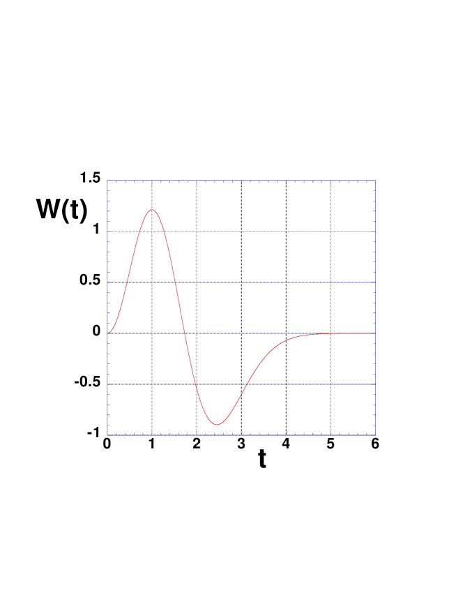
Figure 6: Wavelet kernel used for the wavelet analysis of aftershock diffusion, defined by (13). This wavelet kernel and its derivative both vanish at time $t=0$ and has a zero mean over the interval $[0,+\infty[$.

Our choice of the kernel or mother wavelet $W$ has been dictated by the following considerations. First, the modified Omori law (1) as well as the ETAS model (16) introduce a short-time cut-off $c$ that accounts for seismicity just after the mainshock. Since this cut-off breaks down the exact self-similarity of the Omori kernel, it leads to corrections to the expected diffusion resulting from event triggering cascades at short times [Helmstetter and Sornette, 2002b]. Since $c$ is in general found small, the seismicity rate is very large just after the mainshock which may lead to finite-size and instrumental saturation effects just after the mainshock. In addition, even if these limitations are removed there may be so many aftershocks near $t=0$ that many of them are generally interwoven in seismic recordings, and most of them can not be interpreted and located properly. We thus construct a wavelet kernel $W$ which minimizes the weight given to the seismicity rate at short times after mainshocks. Specifically, we choose the wavelet kernel shown in Figure 6, which vanishes at $t=0$, has also zero time derivative at the origin and has zero average:

$$W(t)=(3t^{2}-t^{4})\exp(-\frac{t^{2}}{2})~{}.$$ (13)

This kernel looks like an aliased sine function. This wavelet kernel is reasonably well localized both in time and scale and its simple expression allows for fast computations on large data sets. The time unit shown in this figure 6 has no special meaning since our wavelet analysis is using scale ratios rather than on absolute scales. Note that the chosen wavelet kernel has properties quite different from those, for instance, of the classical Mexican hat wavelet, widely used in the analysis of singularities, which has a maximum amplitude at $t=0$, and would thus be inappropriate for the reasons listed above.

This choice of the wavelet kernel leads to the decay of the wavelet coefficients $C_{a}(R)\sim 1/a^{3}$ at large times after the last events in the catalog, thus giving an apparent Omori exponent $p=3$. As we know by experience that the Omori exponent is smaller than $2$, an exponent $p=3$ will thus be interpreted as spurious and due to the limited duration of the catalog. This asymptotic property, which is very different from the Omori law we are studying, is a desirable property of the wavelet kernel (13) which provides a clear signal of a possible problem in the data analysis. For example, if no event is present in the catalog between times $t_{1}$ and $t_{2}$, and provided that $t_{2}$ is sufficiently larger than $t_{1}$, then we will measure a spurious $p=3$ for time scales $a$ larger than $t_{1}$ and lower than $t_{2}$. This may lead to some bias in the determination of $p$, that we shall come back to in the discussion.

4.4 Synthetic tests

The determination of the exponents $p$ and $H$ is performed by two algorithms described in Appendix B. This first (respectively second) algorithm uses the $1/H$-scaling (respectively $H$-scaling law) normalized curves.

We have performed tests of the wavelet method on synthetic catalogs generated using the ETAS model and various modifications thereof, with and without genuine diffusion and with or without background seismicity. A particular result is that the wavelet method works better the larger the background noise, up to the point where the meaningful signal would disappear. While for large catalogs with a significant background component, the wavelet method is superior to the windowing method by providing more precise values of $p$ and $H$, it turns out to be inferior to the windowing method for synthetic catalogs without background when catalogs have limited sizes, as it exhibits significant scatter in the determination of the exponents $p$ and $H$. Technically, this scatters occurs due to the existence of large oscillations in the dependence of the wavelet coefficients as a function of $R$ and/or $a$, which makes difficult the determination of the relevant scaling intervals. This paradoxical result reflects the larger sensitivity of the wavelet method to the size of catalogs due to its intrinsic two-dimensional nature, while the windowing method is more robust for small catalogs due to its one-dimensional structure.

Comparing the $H$-method with the $1/H$-method, we note that, due to the fact that the $H$-method uses original curves and not their fit approximations (and are thus more subjected to fluctuations), the “variance landscapes” defined in Appendix B exhibit much more elongated valleys around minima than with the $1/H$-method. As will be shown below, both methods most often yield the same results, but the $1/H$-method yields better-defined minima and should be preferred in general.

4.5 Results

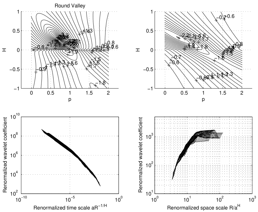
Figure 7: Determination of the exponents $H$ and $p$ for the Round Valley mainshock using the $1/H$-scaling method (upper and lower left panels) and the $H$-scaling method (upper and lower left panels). The upper panels represent the contour plots in $\log_{10}$ scale of equi-values of the average variance of the matching of wavelet coefficients (calculated as a function of time scale for different distances $R$; see text for details) as a function of trial values of $p$ and $H$. The minimum determines our best estimation for $H$ and $p$ for this sequence. We get two estimates, one using the $H$-scaling method ($p=0.35$, $H=0.32$) and another using the $1/H$-scaling method ($p=0.72$, $H=0.24$). Note that the minimum found by the $1/H$-scaling method is better defined than when using the $H$-scaling method. The lower panels show the resulting quality of the collapsed wavelet coefficients as a function of time scale for different distances $R$, using these best estimates of $p$ and $H$.

Table LABEL:tab2wavelet summarizes the results on the values of $p$ and $H$ obtained from the wavelet analysis applied to 21 large earthquakes in California. These events are the same as those studied with the windowing method and reported in Table LABEL:tabdifobs. Table LABEL:tab2wavelet shows that results obtained with the two methods based on the $H$-scaling law and $1/H$-scaling law compare rather well, except for four cases: Westmorland, Round Valley, North Palm Springs, Mammoth Lakes. However, for each earthquake, a detailed analysis of the corresponding contour lines of the average variance of the collapse of wavelet coefficients (see Figure 7 for the Round Valley mainshock) shows that the $1/H$-scaling law method is in general more reliable with a more constrained and better defined minimum. We thus tend to believe the $p$ and $H$ values given by the $1/H$-method as more reliable.

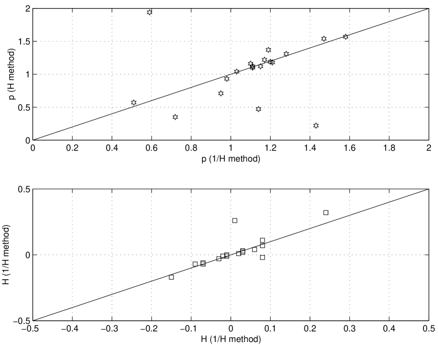
Figure 8: Upper panel: correlation between the Omori exponent $p$ obtained with the $1/H$ method (horizontal axis) and with the $H$ method (vertical axis). The line of slope $1$ is drawn as a reference. Lower panel: correlation between the exponents $H$ obtained with the $1/H$ method (horizontal axis) and with the $H$ method (vertical axis). The line of slope $1$ is drawn as a reference.

Figure 8 shows the correlation between the exponents $p$ and $H$ obtained for each shock. There is a good consistency between both methods. Strictly speaking, negative values of $H$ are associated with “anti-diffusion”, that is, migration of aftershocks towards the mainshock. One possible reason for our finding of negative $H$’s is a spurious bias due to the mismatch between the mainshock epicenter and the barycenter of the aftershock cloud.

5 Discussion

5.1 General synthesis

Our main conclusion is that, in contrast with previous claims, diffusion of aftershocks is in general absent or very weak, at the borderline of detection. This conclusion is reached notwithstanding our significant efforts to develop two independent techniques which have been optimized for extracting a signal on diffusion in the presence of background noise. Maybe, to be fair, we should state more correctly that our rather negative conclusion is reached precisely because we have made large efforts to remove spurious signals. As many tests have shown, some of which presented in section 2, it is easy to construct a diffusion signal in the form of a power law of the characteristic size of the aftershock cloud as a function of time. Our present work has stressed the importance of not jumping to conclusions and that serious tests should be performed to assess the reliability of a putative diffusive power law. The simplest explanation is often that such a power law is due to cross-over effects in the presence of inhomogeneity of the catalogs, of their limited sizes and of the contagion induced by background and uncorrelated seismicity. We also note that most sub-diffusion exponents $H$ reported in previous studies as well as in the present one are very small, in the range $0.05-0.2$. For instance, a value $H=0.1$ implies that ten decades in time scales are needed for each decade in space scale. This “small exponent curse” is one of the many explanations for the difficulty in obtaining a clear-cut diffusion signal.

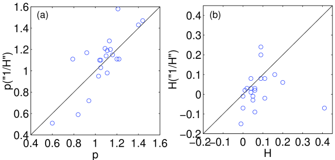
Figure 14: Comparison of the two methods of estimation of $p$ and $H$. (a) Omori exponent measured by the wavelet $1/H$ method (Table 2) versus the Omori exponent estimated by the windowing method (Table 1). (b) Diffusion exponent measured by the wavelet $1/H$ method (Table 2) versus the diffusion exponent $H_{r}$ estimated by the windowing method (Table 1).

Figure 14 compares the values of $p$ and $H$ obtained by the two methods given in Tables 1 and 2. The results for $H$ are essentially uncorrelated between the two methods. Considering they belong to the same aftershock sequences, this supports the conclusion that the diffusion coefficients are not on the whole statistically significant.

Having said that, Tables 1 and 2 show that a few aftershock sequences exhibit a significant and unambiguous diffusion. In order to aggregate the information derived from the windowing and wavelet methods, we compare the exponent $H_{b}$ for the former and the exponent $H$ obtained from the $1/H$-scaling method for the latter and qualify the existence of diffusion (somewhat arbitrarily) when the two criteria $H_{b}\geq 0.1$ and $H_{1/H}\geq 0.05$ are simultaneously verified. Comparing these two methods, six clear-cut cases emerge: Westmorland ($H_{b}=0.12$, $H_{1/H}=0.10$), Morgan-Hill ($H_{b}=0.44$, $H_{1/H}=0.08$), Round-Valley ($H_{b}=0.11$, $H_{1/H}=0.24$), Superstition-Hill ($H_{b}=0.10$, $H_{1/H}=0.06$), Joshua Tree ($H_{b}=0.27$, $H_{1/H}=0.08$) and Mammoth Lakes ($H_{b}=0.16$, $H_{1/H}=0.20$). For the other sequences, either both windowing and wavelet analyses give a very small $H$ or they strongly disagree with each other. The reason for the disagreement between the two methods when it occurs is not obvious to us. With a single method, one can quantify its systematic errors. Using two distinct methods and comparing them enables us to quantify the uncertainties resulting from causes that are difficult to assess a priori. This is our main justification for developing two distinct methods and for comparing their results. We note that such a strategy of using several models emphasizing different physical mechanisms with distinct implementations is well-known and largely used in meteorological forecasts, precisely with the aim of accounting for the unknown or non-understood sources of uncertainties.

It may be helpful to put these results in the light offered by the ETAS model [Helmstetter and Sornette, 2002b] whose main predictions are summarized in Appendix A. The most robust prediction is that one should expect aftershock diffusion when the Omori’s exponent $p$ is less than $1$, because this value signals the existence of a cascade of triggering which is the mechanism at the origin of diffusion in the ETAS model. In the above list of $6$ clear-cut cases, three (Morgan-Hill, Round-Valley and Mammoth Lakes) have an exponent $p$ smaller than $1$ according to both methods, while the three others have a $p$-value larger than or very close to $1$. This fifty-fifty deadlock seems to discredit the usefulness of the ETAS model for this problem. It may be useful to look in more detail at the results of each method separately.

5.2 Discussion of the results in the light of the ETAS model

Most sequences shown in Table 1 for the windowing method and in Table 2 for the wavelet method are in the regime $p>1$ and are characterized by $H\approx 0$. These results are compatible with the predictions of the ETAS model that no diffusion should be observed if the Omori exponent is larger than $1$. Indeed, a measured value $p>1$ can be interpreted as belonging to the sub-critical regime $\nu<1$ (where $\nu$ is the average number of events triggered per triggering event) such that the characteristic time $t^{*}$ defined by (17) is small and the relevant time window covers mostly the regime $t>t^{*}$ for which the cascade process is exhausted and diffusion is absent (Appendix A).

As seen in Table 1 for the windowing method and in Table 2 for the wavelet method, a few aftershock sequences are characterized by a small $p<1$ exponent. As we have said, according to the ETAS model (see Appendix A), this is the relevant regime for observing aftershock diffusion.

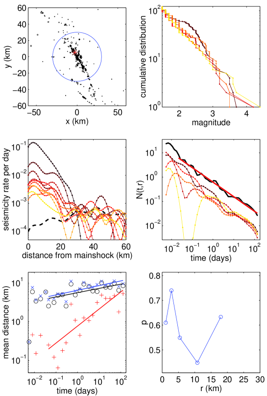
Figure 9: Analysis of the Morgan-Hill aftershock sequence. Same legend as in Figure 3.

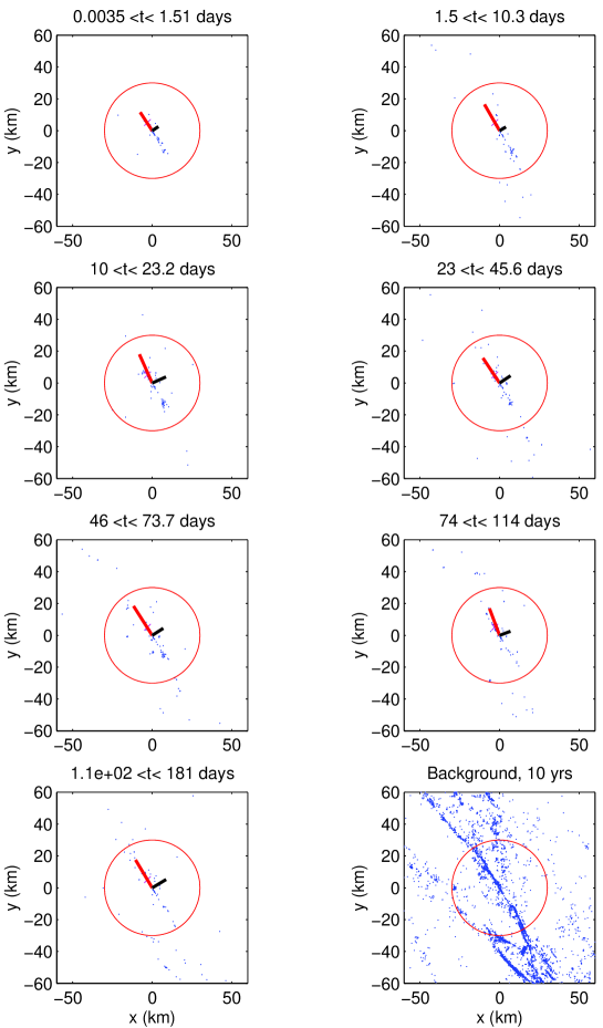
Figure 10: Map of the Morgan-Hill aftershock sequence. Same legend as in Figure 4.

The Morgan-Hill sequence, analyzed in Figures 9 and 10 and which has the smallest $p$-value with both the windowing method ($p=0.6$) and the $1/H$-wavelet method ($p=0.5$), has a small but significant diffusion exponent measured with the windowing method. We obtain $H_{r}\approx H_{a}\approx 0.1$ estimated by the aftershock distances from the barycenter or the large elliptical axis, and a large value $H_{b}=0.44$ obtained by using the time evolution of the small elliptical axes $b$ which measures the average distance of aftershocks from the rupture plane. The value of $H=0.08$ obtained by the wavelet $1/H$-method is similar. The larger value $H_{b}=0.44$ could be due to the fact that the diffusion perpendicular to the fault is less perturbed by the aftershocks along the whole length of the fault which occur in absence of genuine diffusion. For this aftershock sequence, the empirically determined values of $p=0.6$ and $H_{b}=0.44$ would correspond for instance to $\theta\approx 0.4$ and $\mu\approx 1$ (see equation (Appendix A: Summary of main results of the ETAS model concerning aftershock diffusion)) according to the ETAS model [Helmstetter and Sornette, 2002b], where $\theta$ and $\mu$ are defined in equation (16) in Appendix A.

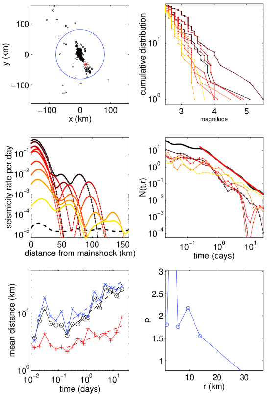
Figure 11: Analysis of the Imperial Valley aftershock sequence. Same legend as in Figure 3.

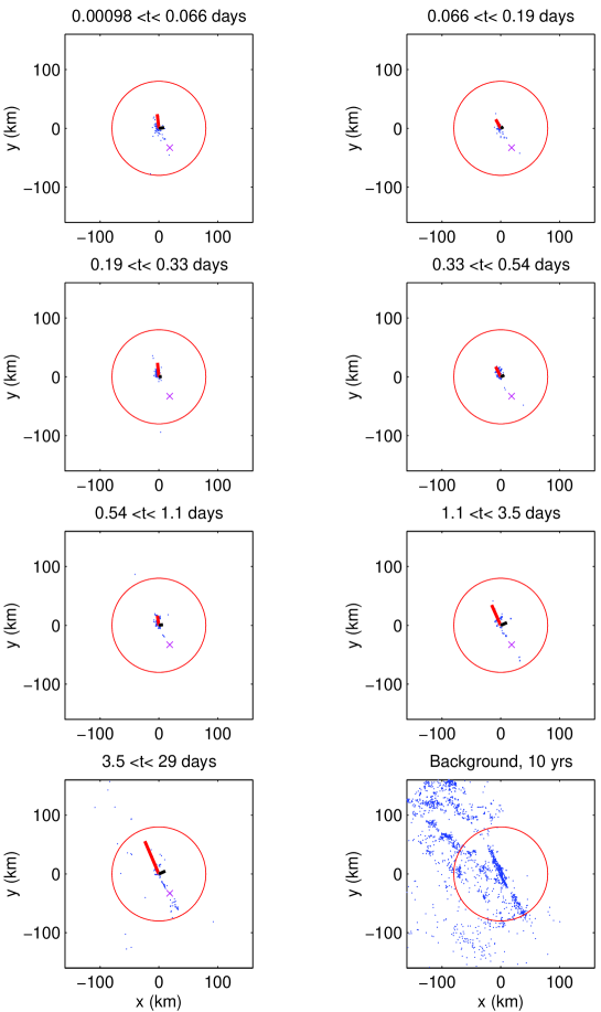
Figure 12: Same as Figure 4 for the Imperial Valley aftershock sequence. Note that the epicenter shown as a cross is far off from the locations where aftershocks cluster. This justifies our use of the aftershock barycenter as a more natural reference point for measuring diffusion.

The other sequences in Table 1 with $p<1$ for which the cascade model predicts the existence of diffusion are Kern-County, Round-Valley, Oceanside and Mammoth Lakes (see table LABEL:tabdifobs for the corresponding parameters). Except for Oceanside, the corresponding $p$ and $H_{b}$ values are compatible with the prediction of the ETAS model [Helmstetter and Sornette, 2002b] with $\mu\approx 1$ leading to $H_{b}\approx 1-p$. While these results are suggestive for the validity of the ETAS predictions, more disturbing is the fact that large values of the diffusion exponents $H$ are found for $p>1$ (see Table LABEL:tabdifobs). The Imperial Valley sequence is a case in point, with the largest $p=1.44$ and large diffusion exponents $H_{r}=0.41,H_{a}=0.37$ and $H_{b}=0.19$. Its detailed analysis is shown in Figures 11 and 12. For this sequence, one can clearly observe an expansion of the aftershock area when comparing the distance distribution at different times. There is also a clear decrease of the exponent $p$ with $r$ as predicted by the ETAS model as a signature of the aftershock cascade leading to diffusion, but this should be associated with $p<1$ and not with $p>1$ as found here. It is true that a significant diffusion exponent $H>0$ with $p>1$ can be observed in the ETAS model in the crossover regime for $t\approx t^{*}$ where $p$ is already larger than 1, but where a diffusion of seismic activity is still observed. Indeed, synthetic aftershock sequences in the sub-critical regime exhibit a diffusion of seismic activity which persists up to $t\approx 100~{}t^{*}$ even if the Omori exponent in larger $1$. But the diffusion exponent $H$ in the crossover regime for $t\approx t^{*}$ should be smaller than in the early time $t<t^{*}$ regime when $p$ is smaller than $1$. We thus do not fully understand the origin of this discrepancy.

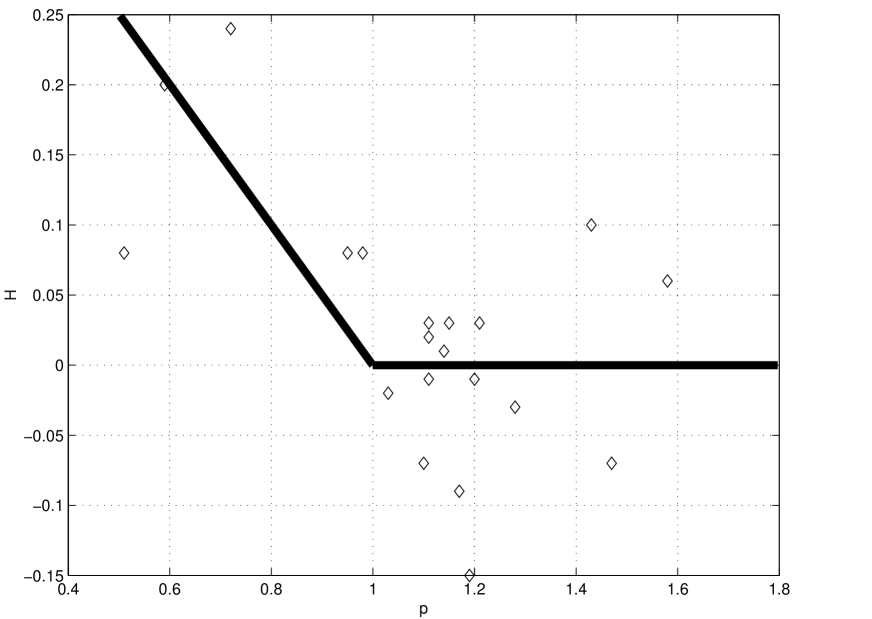
Figure 13: Diffusion exponent $H$ as a function of the Omori law exponent $p$ obtained with the $1/H$ method for all the aftershock sequences described in table LABEL:tab2wavelet. The thick lines are the approximative predictions of the ETAS model for $\mu\geq 2$ (Appendix A: Summary of main results of the ETAS model concerning aftershock diffusion), assuming that $p=1-\theta$ if $p<1$ and $p=1+\theta$ if $p>1$.

Using the wavelet method, only five sequences are in the regime $p<1$ where diffusion is predicted to occur according to the ETAS model and, there, the expected correlation is weak and noisy. The evidence of aftershock diffusion is very weak as $75\%$ of the aftershock sequences seem to be in the non-critical regime ($t>t^{*}$ and $p>1$) characterized by an absence of diffusion. The remaining five sequences are loosely compatible with the existence of diffusion and the quantitative values are consistent with the predictions of [Helmstetter and Sornette, 2002b], when taken collectively. Figure 13 tests the possible existence of a correlation between the diffusion exponent $H$ and the Omori law exponent $p$ obtained with the $1/H$ method for all the aftershock sequences described in table LABEL:tab2wavelet. The thick lines are the prediction of the ETAS model [Helmstetter and Sornette, 2002b] that $H\approx 0$ for $p>1$ and $H=(1-p)/2$ for $p<1$, obtained by choosing $\mu\geq 2$ and by assuming $p=1-\theta$ (which is correct if $t\ll t^{*}$). In the five cases with $p<1$, we find positive exponents $H$ in the range from $0.08$ to $0.24$. A linear fit over these five events with $p<1$, forced to pass through the “origin” $(p=1,H=0)$ gives $H=(p-1)/2.52$, which must be compared with the prediction $H=(1-p)/2$. In the other 15 cases with $p>1$, $H$ is very noisy with almost as many negative and positive values in the range from $-0.15$ to $0.1$, and almost vanishing average.

In conclusion, the results obtained with the two methods do not show any significant correlation between $H$ and $p$, in contradiction with the prediction of the ETAS model. This disagreement between the observations and the theory may result from the insufficient number of aftershocks available. The small number of events used yields a large uncertainty of the measure of $H$ and $p$, as shown by the large difference in the value of $p$ and $H$ obtained for some sequences using the different methods (windowing, $H$ and $1/H$ wavelet method). In addition, these are other factors, such as the fact that the typical mainshock-aftershock distance increases with the mainshock magnitude, or the geometry of the rupture, which are taken into account neither in the ETAS model nor in the empirical analysis, but which may significantly alter the results.

6 Factors limiting the observation of diffusion

This section examines important limitations of both the theoretical analysis of Helmstetter and Sornette [2002b] and our present study of California seismicity and discusses possible remedies.

6.1 Independence between the mainshock size and the aftershock cluster size and selection rules

A limitation of the analytical approach developed in [Helmstetter and Sornette, 2002b] is that the distribution of distances between a mainshock and its aftershocks are assumed independent of the mainshock magnitude. However, it is a well established property of aftershock sequences that the size of the aftershock area is approximately proportional to the mainshock rupture length [Utsu, 1961; Kagan, 2002].

We can modify the ETAS model to include a dependence between the mainshock magnitude and the aftershock size, as observed in real seismicity, in order to take into account the extended rupture length of the mainshock. In this goal, we modify the distance distribution $\sim 1/(r+d)^{1+\mu}$ defined in (16) of Appendix A by taking the characteristic size $d(M)$ proportional to the mainshock rupture length $d(M)\propto L\sim 10^{0.5M}$. This means that an aftershock of generation $i$ is created by an aftershock of generation $i-1$ of magnitude $M_{i-1}$ at a distance $r$ from it via the rate (16) with the distance distribution $\sim 1/(r+d(M_{i-1}))^{1+\mu}$.

We can understand intuitively the effect of introducing a dependence between $d$ and the magnitude, knowing the solution $N(t,r)$ given by Helmstetter and Sornette [2002b] for a constant $d$-value. Starting from a mainshock of magnitude $M$ at the origin, the typical distance between aftershocks of the first generation and the mainshock is $d(M)\propto L$, where $L$ is the rupture length of the mainshock. Aftershocks of second and later generation have a smaller magnitude on average, otherwise they do not qualify as aftershocks of the first event, by our present definition. We can thus define an average rupture size $\langle\ell\rangle<L$ for the aftershocks. As long as the average size of the aftershock zone $R(t)$ is smaller than $L$, the aftershocks of the first generation dominate the spread of seismic activity following the mainshock and diffusion is not observable. At large times, when the aftershock area of second and later generations becomes larger than the influence zone of the mainshock of size $L$ and when most aftershocks are triggered indirectly by aftershocks of the mainshock, the diffusion for the coupled model should be the same as for the decoupled model studied in [Helmstetter and Sornette, 2002b]. The dependence of $d$ with the progenitor’s magnitude thus introduces a crossover time $\tau$ such that there is no significant diffusion below $\tau$ because the aftershock spatial expansion is dominated by aftershocks of the first generation while for time larger than $\tau$ the multiple cascades of aftershocks dominates the spatial excursion of aftershocks and we recover the diffusion law (5) of the decoupled model. This gives the equation for $\tau$:

$$\langle\ell\rangle\Bigl{(}{\tau\over c}\Bigr{)}^{H}\approx L~{},$$ (14)

leading to

$$\tau=c\left({L\over\langle\ell\rangle}\right)^{1/H}$$ (15)

where $L$ is the mainshock size and $\langle\ell\rangle$ is the average rupture length of aftershocks. For large mainshocks $L\gg\langle\ell\rangle$ and slow diffusion, this characteristic time $\tau$ can be very large and, in practice, diffusion may be unobserved in real aftershock sequences.

6.2 Rules of aftershock selection

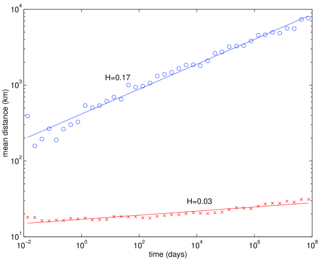
Figure 15: Average distance $R(t)$ between a mainshock of magnitude $M=6$ and its aftershocks for numerical simulations of the ETAS model with $n=1$, $\alpha=0.5$, $b=1$, $c=0.001$, $\theta=0.2$, $m_{0}=0$ and $\mu=1$, obtained by averaging over 1000 simulations. The circles show the results for $d=10$ km, independently of the mainshock size, and without any constrain on aftershock selection. The diffusion exponent $H=0.17$ is close to the prediction $H=\theta/\mu=0.2$. The crosses correspond to another simulations of the ETAS model with the same parameters except that the characteristic distance $d$ now depends on the magnitude of each event according to $d=0.01^{0.5M}$. For this simulation, we have also selected aftershocks up to a distance of 100 km (10 times the mainshock rupture length) and we have rejected all aftershock sequences containing at least an event larger than the mainshock. All these factors weaken the diffusion by comparison the the prediction of the ETAS model.

There are two other factors that may further weaken the observed diffusion in comparison with the prediction of the ETAS model given in [Helmstetter and Sornette, 2002b]. First, the constraint that the aftershocks must be smaller than the mainshock induces an under-estimation of the true diffusion exponent. If we include this rule of aftershock selection in the numerical simulations, the average seismicity rate is smaller than the predicted seismicity rate and decreases as $1/t^{1+\theta}$ at large times instead of the theoretical prediction $N(t)\sim 1/t^{1-\theta}$ for $t<t^{*}$ or $n=1$. This effect induces a slower diffusion at large times when the observed Omori exponent becomes larger than 1. The other factor which may lower the diffusion in the real aftershock sequence is the introduction of a maximum distance $r_{max}$ for the selection of aftershocks close to the mainshock. Introducing this rule in the simulations of the ETAS model obviously lowers the diffusion exponent by comparison with the true exponent, because it rejects all aftershocks triggered at large distance from the mainshock which have an important role in the diffusion process, especially for small value of $\mu<2$. The effect of the rupture geometry and the rules of aftershock selection are illustrated in Figure 15 for numerical simulations of the ETAS model obtained for $\alpha=0.5$, $b=1$, $n=1$, $\mu=1$, $c=0.001$ day, $m_{0}=0$, $M=6$, $d=0.01\times 10^{0.5M}$ km. This Figure shows that the combined effect of the dependence between the influence distance $d$ and the rupture length $L$, and the rules of aftershock selection results in a strong reduction of the diffusion in comparison with the predictions given in [Helmstetter and Sornette, 2002b].

6.3 Influence of the fault geometry

Another important limitation of the ETAS model and of other models of aftershocks such as the rate-and-state friction model [Dieterich, 1994] is that these models do not take into account the anisotropy of the spatial distribution of aftershocks nor the localization of earthquakes on a fractal fault network. These factors may also have an important influence on aftershock diffusion.

There is strong evidence that earthquakes occur on faults and faults are organized in a complex hierarchical network [Ouillon et al., 1996]. A simplified representation of this network uses fractal geometry. A better description of aftershock diffusion, if any, should thus deal with the problem of diffusion on a fractal network. Some general results have been obtained in the physical literature on this problem of diffusion of probe particles in non-Euclidean fractal spaces (see Bouchaud and Georges [1990], Sahimi [1993; 1994] and references therein). The main consequence is that the diffusion exponent $H$ may be modified to take into account the fractal geometry through the introduction of the so-called spectral dimension (which is often different from the geometrical fractal dimension). In general, this leads to reduced diffusion when measured with Euclidean distances. Another possible caveat is the anisotropy of fault networks, resulting from the localization properties of mechanical systems which tend to organize oriented shear bands. For instance, there is a very strong South-East to North-West preferred orientation of the San Andreas fault network in California.

While previous empirical analyses including the present one as well as the ETAS model of cascades of triggering have neglected geometry, our tests suggest that geometry is a crucial ingredient. By geometry, one should include both the effect of a possible localization of a fraction of aftershocks on mainshock rupture faults and their localization of pre-existing hierarchical fault networks, as well as the dependence of the range over which aftershocks are triggered by the mainshock on the mainshock magnitude.

7 Conclusion

We have analyzed 21 aftershock sequences of California and found that the diffusion of seismic activity is very weak, when compared with previous studies. For most sequences, the spatial distribution of aftershocks is mostly limited to the mainshock rupture area. The rate of aftershocks is very small at distances larger than the rupture length, even at large times after the mainshock.

In the introduction, we noted that aftershock diffusion is predicted by any model that assumes that the time to failure increases if the applied stress decreases. Our conclusion that aftershock diffusion is weak at best or non-existent suggests that the physical process controlling the time of failure depends weakly on the magnitude of the stress change in the regime where this stress change is sufficient to trigger new events.

We have examined the hypothesis that aftershock diffusion may result from multiple triggering of secondary aftershocks. In principle, this mechanism offers clear quantitative predictions, if one controls the parameter regime of the model. One problem is that our theoretical and numerical studies of cascade processes indicate that most predictions are very sensitive to small changes in the parameters of the seismic activity which cannot be easily determined from seismicity catalogs. This variability of the ETAS parameters from sequence to sequence may thus rationalize the variability of the diffusion exponent from one sequence to another one. In conclusion, the large uncertainty on the estimation of the Omori exponent $p$ and the diffusion exponent $H$, resulting from different factors (small number of events, small available time and space scale, background seismicity and fault geometry, high fluctuations from one sequence to another one), does not allow us to conclude clearly the validity or the irrelevance of the mechanism of triggering cascade embodied by the ETAS model in describing aftershock diffusion.

We thank D. Marsan for providing his code and the preprints of his papers and for several exchanges and J.-R. Grasso for useful discussions. This work is partially supported by NSF-EAR02-30429, by the Southern California Earthquake Center (SCEC) and by the James S. Mc Donnell Foundation 21st century scientist award/studying complex system. We acknowledge SCEC for the earthquake catalogs.

Appendix A: Summary of main results of the ETAS model concerning aftershock diffusion

The ETAS (Epidemic-Type Aftershock Sequence) model was introduced in Ogata [1988] and in Kagan and Knopoff [1981; 1987] (in a slightly different form) based on mutually exciting point processes introduced by Hawkes [Hawkes, 1971; 1972; Hawkes and Adamopoulos, 1973]. Contrary to what its name may imply, it is not only a model of aftershocks but a general model of triggered seismicity.

This parsimonious physical model of multiple cascades of earthquake triggering avoids the division between foreshocks, mainshocks and aftershocks because it uses the same laws to describe all earthquakes without distinction between foreshocks, mainshocks and aftershocks. It is found [Helmstetter and Sornette, 2002a,b,c; 2003a; Helmstetter et al., 2003] to account surprisingly well for (i) the increase of rate of foreshocks before mainshocks (ii) at large distances and (iii) up to decades before mainshocks, (iv) a change of the Gutenberg-Richter law from a concave to a convex shape for foreshocks, and (v) the migration of foreshocks toward mainshocks. The emerging concept is that the cascade of secondary, tertiary and higher-level triggered events gives rise naturally to long-range and long-time interactions, without the need for any new physics. This emphasis on cascades of triggered seismicity provides a general understanding of the space-time organization of seismicity and offers new improved methods for earthquake prediction.

In the ETAS model, a main event of magnitude $m$ triggers its own primary aftershocks according to the following distribution in time and space

$$\phi_{m}(r,t)~{}dr~{}dt=K~{}10^{\alpha m}~{}\frac{\theta~{}c^{\theta}~{}dt}{(t+c)^{1+\theta}}~{}\frac{\mu~{}d^{\mu}~{}dr}{(r+d)^{1+\mu}}~{},$$ (16)

where $r$ is the spatial distance to the main event (considered as a point process). The spatial regularization distance $d$ accounts for the finite rupture size. The power law kernel in space with exponent $\mu$ quantifies the fact that the distribution of distances between pairs of events is well described by a power-law [Kagan and Jackson, 1998]. In addition, the magnitude of these primary aftershocks is assumed to be distributed according to the Gutenberg-Richter law with slope $b$. The ETAS model assumes that each primary aftershock may trigger its own aftershocks (secondary events) according to the same law, the secondary aftershocks themselves may trigger tertiary aftershocks and so on, creating a cascade process. The exponent $1+\theta$ is not the observable Omori exponent $p$ but defines the local (or direct) Omori law. The whole series of aftershocks, integrated over the whole space, can be shown to lead to a “renormalized” (or dressed) Omori law, which is the total observable Omori law [Helmstetter and Sornette, 2002a]. This global law is different from the direct Omori law $1/(t+c)^{1+\theta}$ in (16): the observable (dressed) Omori exponent crosses over smoothly from the value $1-\theta$ below a characteristic time $t^{*}$ to $1+\theta$ at times much larger than $t^{*}$

$$t^{*}=c~{}\left({\nu~{}\Gamma(1-\theta)\over|1-\nu|}\right)^{1/\theta}$$ (17)

where the branching ratio $\nu$, defined as the average number of aftershocks per earthquakes, is a function of the parameters of the ETAS model $\nu=K~{}b/(b-\alpha)$. The renormalization of the direct Omori law with exponent $1+\theta$ into the observable dressed Omori law with exponent $1-\theta$ (for $t\leq t^{*}$) results from the cascade process. Intuitively, it is clear that the existence of cascades of secondary aftershocks may lead to observable diffusion, analogously to random walks whose succession of jumps create diffusion upon averaging. This analogy was established in [Helmstetter and Sornette, 2002b] which predicted different diffusion regimes according to the values of the model parameters. The simplest mathematical characterization of diffusion is through the evolution of the characteristic size $R$ of the aftershock cloud as a function of time $t$ since the main shock:

$$R\sim t^{H}~{},$$ (18)

where $H$ is the diffusion exponent (equal to $1/2$ for classical diffusion). The theory and numerical simulations developed in [Helmstetter and Sornette, 2002b] predict, for $t<t^{*}$ and $\theta<1$ :

$$H = \theta/2~{}~{}~{}\mbox{for}~{}~{}\mu>2$$ (19)

$$H = \theta/\mu~{}~{}~{}\mbox{for}~{}~{}\mu<2~{}.$$

where

$$r^{*}=\sigma\left({\nu\over 1-\nu}\right)^{1/\mu}~{},$$ (20)

and $\sigma$ is proportional to the spatial regularization distance $d$ in (16) up to a numerical constant function of $\mu$ [Helmstetter and Sornette, 2002b]. In all cases, the diffusion saturates progressively as $t$ becomes much larger than $t^{*}$. Here, the important message is that, despite the fact that time and space are uncoupled in the direct triggering process (16), the succession of cascades of events can lead to a macroscopic coupling of time and space, that is, to diffusion. This is illustrated in Figure 1 which presents results from numerical simulations of the ETAS model to show how cascades of multiple triggering can produce aftershock diffusion. Since the condition $t<t^{*}$ also ensures that the observable Omori exponent $1-\theta$ is different from the direct exponent $1+\theta$, this triggering cascade theory predicts that diffusion should be observed most clearly when Omori’s exponent $p$ is smaller than $1$. Note that, for $p$ close to $1$ as often observed empirically, that is for $\theta$ small, the predicted diffusion exponent $H$ is significantly smaller than $1/2$. The results in [Helmstetter and Sornette, 2002b] were obtained for a one dimensional process, but most results, in particular the diffusion law (18), are valid in any dimension. Another complication elaborated upon below is the fractal geometry of fault networks.

A possible caveat in the predictions of the ETAS model given in [Helmstetter and Sornette, 2002b] is that we predict only the average behavior of the space-time distribution of seismicity. In the regime where $\alpha/b>0.5$ relevant to real seismicity [Helmstetter, 2003], we observe huge fluctuations of the seismicity rate around the average that may weaken the usefulness of predictions based on ensemble averages. Having said that, we have verified by intensive numerical simulations that the prediction $H\geq(1-p)/2$ remains valid in all cases including the large deviation regime $\alpha>b/2$. Thus, for the problem treated here of detecting a possible aftershock diffusion, this issue is not a limiting point.

Our tests on real aftershock sequences are interpreted in particular in the light shed by the ETAS model. We stress that the analysis of real data is much more difficult than the study of synthetic sequences, due to the smaller number of earthquakes available, the presence of background activity, the effect of geometry and problems of catalog completeness especially just after large mainshocks. In addition, real seismicity is probably more complicated than assumed by the ETAS model. These limitations imply that it is difficult to obtain reliable quantitative results on the diffusion exponent. However, a few qualitative predictions of the ETAS model should be testable in real data:

• only sequences in the “early” time regime $t<t^{*}$ characterized by an Omori exponent $p<1$ should diffuse;

• the diffusion of seismic activity should be related to a decrease of the Omori exponent $p$ as the distance $r$ from the mainshock increases;

• the characteristic size of the cluster is expected to grow according to expression (18) with the diffusion exponent $H$ positively correlated with the $\theta$-value.

Appendix B: Implementation of the wavelet method

Method using the $1/H$-scaling law normalized curves

The determination of the exponents $p$ and $H$ is performed by using the following steps when using the $1/H$-scaling law normalized curves:

1. Compute $C_{a}(R)$ as a function of scale $a$ for a series of given $R$ values. Typically, we considerer $a$ values varying with a multiplicative factor of $1.1$, while $R$ varies with a multiplicative factor of $1.01$. This last value will be justified below. For each $R$ value we thus obtain a curve showing the variation of $C_{a}(R)$ with $a$. Those curves are called $R$-curves.

2. Select the range in scale $a$ over which all $R$-curves display a power-law behavior as a function of $a$. Note that the exponent of the power law may vary from one $R$ to another $R$ (which is the hallmark of an underlying diffusion process). We could also select a different range of $a$ for each value of $R$, but this would drastically complicate the data processing.

3. For each $R$-curve, fit $C_{a}(R)$ over the selected range in $a$ by a power law. This step proves necessary as some data sets can sometimes display strong fluctuations which will ultimately alter the results (this has been checked on synthetic data sets). Each interval in $a$ for each $R$-curve is now replaced by its power-law fit approximation.

4. Choose a trial $(p,H)$ and normalize each curve according to these exponents and their respective $a$ and $R$ values according to (12) ($1/H$-scaling law). The normalized time scale axis is then re-sampled using a geometrical sampling with a multiplicative factor of $1.1$, so that all normalized R-curves are defined at common abscissae.

5. For each normalized value of the time scale, search for all normalized power law approximations of $R$-curves which are defined at that value. Let us assume there are $N_{s}$ such segments, each one corresponding to a different $R$-curve (thus $R$ value).

6. Compute the average value of these normalized $R$-curves that are defined at the same normalized time scale, as well as the associated variance. If none or only one power law approximation of $R$-curves is defined for the considered normalized time scale, the calculation is not performed as the variance cannot be estimated. Then, go to the next normalized time scale.

7. When all values of the normalized time scale have been considered, compute the average of all the variances that have been defined up to now. This average variance gives us an estimation of how the various normalized segments collapse on top of each other in the goal of defining a single master curve. It is approximately equivalent to the square of the average width defined by superimposing all the normalized curves.

8. This algorithm is implemented using a $(p,H)$ grid, with $p$ varying from $0$ to $2$ by steps of $0.01$, while $H$ varies within $[-1:1]$, with the same step. When $H=0$, no computation is made. A systematic search provides the couple of exponents $(p,H)$ with the lowest average variance, i.e., the best collapse of the wavelet coefficients as a function of time scale and distance. For $H=0$, the value of the variance for any couple $(p,0)$ is estimated as the mean of the variances obtained for $(p,-0.01)$ and $(p,0.01)$. This estimation has no real statistical meaning but is useful for representation purpose. The top left panel of Figure 7 constructed for the Round Valley mainshock show the contour lines representing equivalues of the average variance (quantified in logarithmic scale in base $10$).

9. Once the best $(p,H)$ couple has been found, the normalized wavelet coefficients $C_{a}(R)$ are calculated as a function of $a$ using the original non-normalized real curves (and not their power-law fit approximations). This is performed for the purpose of visualizing the predicted collapse of the wavelet coefficients on the real data-set, as shown in the left lower panel of Figure 7 constructed for the Round Valley mainshock.

Note that this collapse method applied to the $1/H$-scaling law can not work for $H=0$ strictly, since $1/H$ diverges. To address this minor technical problem, we choose a very small logarithmic step for the $R$ values to allow us to consider $H$ values as small as $\pm 0.01$. Indeed, the smaller is $|H|$, the more dilated is the normalized time scale axis. If $H$ is too small, the scaling regions of two successive wavelet coefficients for two successive $R$ values will undergo so much offset that they will not be defined on any common normalized time scale, preventing an estimation of an average variance. Considering small values of $H$ thus necessitates the computation of wavelet coefficients for successive $R$ with a very small step in $R$ (hence the choice of a multiplicative factor of $1.01$).

Method using the $H$-scaling law normalized curves

The determination of the exponents $p$ and $H$ is performed by using the following steps when using the $H$-scaling law normalized curves:

1. We now re-organize all the $C_{a}(R)$ values by plotting curves of $C_{a}(R)$ as a function of $R$ for various values of $a$. These are now the $a$-curves.

2. The $a$-curves do not display any peculiar behavior with $R$. They are monotonically increasing with $R$, and saturate at large $R$ values. Among those $a$-curves, there is always a subset of curves which are nearly parallel (or at least don’t cross each other), which is a behavior predicted by diffusive processes. If all the curves are strictly parallel, one can conclude there is no underlying diffusion at all. Other curves either cross this subset, or are simply too noisy and are thus eliminated. This allows us to select the $a$-curves we will use to invert for $p$ and $H$ using the $H$-scaling law. Note that we will conserve “raw” $a$-curves, which can’t be approximated by any power-law.

3. Choose a trial $(p,H)$ and normalize each curve according to these exponents and their respective $a$ and $R$ values according to (11) ($H$-scaling law). The normalized space scale axis is then re-sampled using a geometrical sampling with a multiplicative factor of $1.01$, so that all normalized $a$-curves are defined at common abscissae.

4. For each normalized value of the space scale, search for all normalized $a$-curves which are defined at that value. Let us assume there are $N_{s}$ such segments, each one corresponding to a different $a$-curve (thus $a$ value).

5. Compute the average value of these normalized $a$-curves that are defined at the same normalized time scale, as well as the associated variance. If none or only one $a$-curve is defined for the considered normalized space scale, the calculation is not performed as the variance cannot be estimated. Then, go to the next normalized time scale.

6. When all values of the normalized space scale have been considered, compute the average of all the variances that have been defined up to now. This average variance gives us an estimation of how the various normalized curves collapse on top of each other in the goal of defining a single master curve. It is approximately equivalent to the square of the average width defined by superimposing all the normalized curves.

7. This algorithm is implemented using a $(p,H)$ grid, with $p$ varying from $0$ to $2$ by steps of $0.01$, while $H$ varies within $[-1:1]$, with the same step. When $H=0$, no computation is made. A systematic search provides the couple of exponents $(p,H)$ with the lowest average variance, i.e., the best collapse of the wavelet coefficients as a function of time scale and distance. In this case, there is no problem for $H=0$. The top right panel of Figure 7 constructed for the Round Valley mainshock show the contour lines representing equivalues of the average variance (quantified in logarithmic scale in base $10$).

8. Once the best $(p,H)$ couple has been found, the normalized wavelet coefficients $C_{a}(R)$ are calculated as a function of $R$ using the original non-normalized $a$-curves. This is performed for the purpose of visualizing the predicted collapse of the wavelet coefficients on the real data-set, as shown in the right lower panel of Figure 7 constructed for the Round Valley mainshock.

1

Table 1: Analysis of aftershock sequences of California with the windowing method. The first and second columns give the name and time of the mainshock. $M$ is the mainshock magnitude, $T$ and $R$ are the temporal and spatial windows used to select aftershocks, $M_{0}$ is the minimum magnitude of aftershocks, $p$ is the Omori exponent measured over $t_{min}<t<T$, $N$ is the number of aftershocks. $H_{r}$, $H_{a}$ and $H_{b}$ are the diffusion exponents measured using the average distance between aftershocks and the barycenter, the large elliptical axis $a$, and the short elliptical axis $b$ respectively.

earthquake	date	$M$	$T$	$R$	$M_{0}$	$t_{min}$	$N$	$p$	$H_{r}$	$H_{a}$	$H_{b}$
	(dd/mm/yy)		(days)	(km)		(days)
Kern-County	21/07/52	7.5	5478	70	3.5	1.0	281	0.92	0.06	0.05	0.08
San Fernando	09/02/71	6.6	1096	40	3.0	0.1	274	1.04	0.01	0.03	-0.01
Oroville	01/08/75	5.7	1826	15	2.0	1.0	785	1.09	0.04	0.04	0.04
Imperial Valley	15/10/79	6.4	36	80	2.5	0.2	677	1.44	0.41	0.37	0.19
Westmorland	26/04/81	5.7	73	20	1.7	0.2	587	1.40	0.16	0.16	0.12
Coalinga	02/05/83	6.7	1826	22	2.0	1.0	3133	1.03	0.04	0.04	0.01
Morgan-Hill	24/04/84	6.2	182	30	1.5	0.02	633	0.60	0.11	0.12	0.44
Round-Valley	23/11/84	6.1	182	15	2.0	0.1	1398	0.94	0.09	0.09	0.11
North Palm Springs	8/07/86	5.6	365	15	1.5	1.0	2331	1.10	0.04	0.05	0.04
Oceanside	13/07/86	5.4	3650	20	2.0	0.5	1926	0.79	0.06	0.08	0.02
Chalfant Valley	21/07/86	6.4	1826	20	2.0	1.0	2985	1.16	0.06	0.03	0.16
Superstition-Hill	24/11/87	6.6	18	50	1.8	0.4	794	1.21	0.20	0.20	0.10
Loma-Prieta	18/10/89	7.0	36	50	2.0	0.1	728	1.05	0.11	0.09	0.29
Joshua-Tree	23/04/92	6.1	36	30	1.6	3.0	3658	1.11	0.09	0.03	0.27
Cape Mendocino	25/04/92	6.5	36	70	2.0	0.6	1197	1.20	0.05	0.01	0.13
Landers	28/06/92	7.3	365	60	2.2	3.0	7278	1.05	0.00	-0.01	0.02
Big Pine	17/05/93	6.2	365	25	1.5	2.0	780	1.22	0.02	0.00	0.04
Northridge	17/01/94	6.7	1826	30	2.0	2.0	3254	1.13	0.05	0.06	0.07
Nevada (Carter)	12/09/94	5.5	365	25	2.5	5.0	502	1.11	-0.01	0.05	0.00
Mammoth Lakes	15/05/99	5.6	735	10	1.5	0.2	1570	0.84	0.09	0.07	0.16
Hector-Mine	16/10/99	7.1	1826	35	2.5	1.0	1812	1.14	0.00	-0.01	0.09

2

Table 2: Analysis of aftershock sequences of California with the wavelet method. The first column gives the name of the mainshocks. $p$ ($H$ method) is the Omori’s exponent obtained with the $H$-scaling law. The quantities $a$ and $R$ are discussed in the text. $p$ ($1/H$ method) is the Omori’s exponent obtained with the $1/H$-scaling law. $H$ ($H$ method) is the diffusion exponent obtained with the $H$-scaling law. $H$ ($1/H$ method) is the diffusion exponent obtained with the $1/H$-scaling law.

earthquake	$a$ range	$R$ range	$p$(“$1/H$”)	$p$(“$H$”)	$H$(“$1/H$”)	$H$(“$H$”)
	(days)	(km)
Kern-County	$9.5-73$	$40-150$	$1.17$	$1.22$	$-0.09$	$-0.07$
San Fernando	$2-15$	$5-30$	$1.1$	a	$0.02$	a
Oroville	$110-365$	$4-30$	$1.21$	$1.18$	$0.03$	$0.03$
Imperial Valley	$2-55$	$41-200$	$1.47$	$1.54$	$-0.07$	$-0.07$
Westmorland	$0.75-75$	$5-15$	$1.43$	$0.22$	$0.10$	$0.52$
Coalinga	$3-360$	$3-20$	$0.95$	$0.81$	$0.08$	$0.11$
Morgan-Hill	$0.75-256$	$3-120$	$0.51$	$0.57$	$0.08$	$-0.02$
Round-Valley	$1-30$	$2-20$	$0.72$	$0.35$	$0.24$	$0.32$
North Palm Springs	$2.5-1825$	$2-10$	$1.14$	$0.47$	$0.01$	$0.26$
Oceanside	$1-5.5$	$5-20$	$1.11$	$1.12$	$0.02$	$0.01$
Chalfant Valley	$4-1460$	$3-30$	$1.15$	$1.12$	$0.03$	$0.03$
Superstition-Hill	$2-25$	$5-40$	$1.58$	$1.57$	$0.06$	$0.04$
Loma-Prieta	$0.25-37$	$7-200$	$1.03$	$1.04$	$-0.02$	$-0.01$
Joshua-Tree	$7-26$	$1.7-12$	$0.98$	$0.93$	$0.08$	$0.07$
Cape Mendocino	$3-128$	$12-70$	$1.11$	$1.12$	$-0.01$	$-0.01$
Landers	$15-1100$	$3-180$	$1.10$	$1.16$	$-0.07$	$-0.06$
Big Pine	$3-365$	$5-50$	$1.11$	$1.10$	$0.03$	$0.02$
Northridge	$15-730$	$7-90$	$1.28$	$1.31$	$-0.03$	$-0.03$
Nevada (Carter)	$18-90$	$4-45$	$1.19$	$1.37$	$-0.15$	$-0.17$
Mammoth Lakes	$1-4$	$2-8$	$0.59$	$1.94$	$0.20$	$-0.72$
Hector-Mine	$2-220$	$2-30$	$1.20$	$1.19$	$-0.01$	$0.00$

^a The $H$ and $p$ values cannot be estimated with the $H$-wavelet method for the San-Fernando sequence because there is no clear minimum of the variance.

References

- [Bouchaud and Georges, 1990] Bouchaud, J.-P. and A. Georges, Anomalous diffusion in disordered media: Statistical mechanisms, models and physical applications, Physics Reports, 195, 127-293, 1990.
- [Chatelain et al., 1983] Chatelain, J.L., R.K. Cardwell and B.L.Isacks, Expansion of the aftershock zone following the Vanuatu (New Hebrides) earthquake on 15 July 1981, Geophys. Res. Lett., 10, 385-388, 1983.
- [Das and Scholz, 1981] Das, S. and Scholz, C.H., Theory of time-dependent rupture in the Earth, J. Geophys. Res., 86, 6039-51, 1981.
- [Dieterich, 1994] Dieterich, J., Constitutive law for rate of earthquake production and its application to earthquake clustering, J. Geophys. Res., 99, 2601-2618, 1994.
- [Fukuyama, 1991] Fukuyama, E., Inversion for the rupture details of the 1987 east-Chiba earthquake, Japan, using a fault model based on the distribution of relocated aftershocks, J. Geophys. Res., 96, 8205-8217, 1991.
- [Hawkes, 1971] Hawkes, A.G., Point spectra of some mutually exciting point processes. Journal of Royal Statistical Society, series B 33, 438-443, 1971.
- [1972] Hawkes, A.G., Spectra of some mutually exciting point processes with associated variables, In Stochastic Point Processes, ed. P.A.W. Lewis, Wiley, 261-271, 1972.
- [Hawkes and Adamopoulos, 1973] Hawkes, A.G. and Adamopoulos, L., Cluster models for earthquakes - regional comparisons, Bull. Internat. Stat. Inst., 45, 454-461, 1973.
- [Helmstetter, 2003] Helmstetter, A., Is earthquake triggering driven by small earthquakes? submitted to Phys. Res. Lett., 2003 (http://arXiv.org/abs/physics/0210056).
- [Helmstetter and Sornette, 2002a] Helmstetter, A. and D. Sornette, Sub-critical and supercritical regimes in epidemic models of earthquake aftershocks, J. Geophys. Res., 107, 2237, doi:10.1029/2001JB001580, 2002a.
- [Helmstetter and Sornette, 2002b] Helmstetter, A. and D. Sornette, Diffusion of epicenters of earthquake aftershocks, Omori’s law, and generalized continuous-time random walk models, Physical Review E., 6606, 061104, 2002b.
- [Helmstetter and Sornette, 2002c] Helmstetter, A. and D. Sornette, Predictability in the ETAS model of interacting triggered seismicity, in press in J. Geophys. Res., 2002c (http://arXiv.org/abs/cond-mat/0208597).
- [Helmstetter and Sornette, 2003] Helmstetter, A, and D. Sornette, Foreshocks explained by cascades of triggered seismicity, submitted to J. Geophys. Res. (http://arXiv.org/abs/physics/0210130), 2003.
- [Helmstetter et al., 2003] Helmstetter, A., D. Sornette and J.-R. Grasso, Mainshocks are aftershocks of conditional foreshocks: how do foreshock statistical properties emerge from aftershock laws, J. Geophys. Res., 108, 2046, doi:10.1029/2002JB001991, 2003.
- [Huc and Main, 2003] Huc, M. and I.G. Main, Anomalous stress diffusion in earthquake triggering : correlation length, time-dependence, and directionality, in press in J. Geophys. Res., 2003.
- [Hudnut et al., 1989] Hudnut K.W., L. Seeber and J. Pacheco, Cross-fault triggering in the November 1987 Superstition Hill earthquake sequence, southern California, Geophys. Res. Lett., 16, 199-203, 1989.
- [Imoto, 1981] Imoto, M., On migration phenomena of aftershocks following large thrust earthquakes in subduction zones, Report of the National Research Center for Disaster Prevention, 25, 29-71, 1981.
- [Jacques et al., 1999] Jacques, E, J.C. Ruegg, J.C. Lepine, P. Tapponnier, G.C.P. King, and A. Omar, Relocation of events of the 1989 Dobi seismic sequence in Afar: evidence for earthquake migration, Geophys. J. Int., 138, 447-469, 1999.
- [Kagan, 2002] Kagan, Y.Y., Aftershock zone scaling, Bull. Seismol. Soc. Am., 92, 641-655, 2002.
- [Kagan and Jackson, 1998] Kagan, Y.Y. and D.D. Jackson, Spatial aftershock distribution: Effect of normal stress, J. Geophys. Res., 103, 24453-24467, 1998.
- [Kagan and Knopoff, 1980] Kagan Y.Y. and Knopoff L., Spatial distribution of earthquakes : the two-point correlation function, Geophys. J. R. Astr. Soc., 62, 303-320, 1980.
- [Kagan and Knopoff, 1981] Kagan, Y.Y. and L. Knopoff, Stochastic synthesis of earthquake catalogs, J. Geophys. Res., 86, 2853-2862, 1981.
- [Kagan and Knopoff, 1987] Kagan, Y.Y. and L. Knopoff, Statistical short-term earthquake prediction, Science, 236, 1563-1467, 1987.
- [King et al., 1994] King, G.C.P., Stein, R.S. and Lin, J., Static stress changes and the triggering of earthquakes, Bull. Seismol. Soc. Am., 84, 935-953, 1994.
- [Lee and Sornette, 2000] Lee, M. W. and D. Sornette, Novel mechanism for discrete scale invariance in sandpile models, Eur. Phys. J. B, 15, 193-197, 2000.
- [Marsan et al., 1999] Marsan, D., C. J. Bean, S. Steacy and J. McCloskey, Spatio-temporal analysis of stress diffusion in a mining-induced seismicity system. Geophys. Res. Lett., 26, 3697-3700, 1999.
- [Marsan et al., 2000] Marsan, D., C.J. Bean, S. Steacy and J. McCloskey, Observation of diffusion processes in earthquake populations and implications for the predictability of seismicity systems, J. Geophys. Res., 105, 28,081-28,094, 2000.
- [Marsan and Bean, 2003] Marsan, D. and C.J. Bean, Average dynamical seismicity changes following a stress perturbation, for a world-wide catalogue, in press in Geophys. J. Int., 2003.
- [Mogi, 1968] Mogi K., Sequential occurrences of recent great earthquakes, J. Phys. Earth, 16, 30, 1968.
- [Noir et al., 1997] Noir, J., E. Jacques, S. Bekri, P.M. Adler, P. Tapponnier, and G.C.P. King, Fluid flow triggered migration of events in the 1989 Dobi earthquake sequence of Central Afar, Geophys. Res. Lett., 24, 2335-2338, 1997.
- [Nur and Booker, 1972] Nur A. and J.R. Booker, Aftershocks caused by pore fluid flow? Science, 175, 885-888, 1972.
- [Ogata, 1988] Ogata, Y., Statistical models for earthquake occurrence and residual analysis for point processes, J. Am. stat. Assoc., 83, 9-27, 1988.
- [Ouchi and Uekawa, 1986] Ouchi, T. and T. Uekawa, Statistical analysis of the spatial distribution of earthquakes - variation of the spatial distribution of earthquakes before and after large earthquakes, Phys. Earth Planet. Inter., 44, 211-225, 1986.
- [Ouillon et al., 1996] Ouillon, G., C. Castaing and D. Sornette, Hierarchical scaling of faulting, J. Geophys. Res. 101, 5477-5487, 1996.
- [Rydelek and Sacks, 1990] Rydelek, P.A. and I.S. Sacks, Asthenospheric viscosity and stress diffusion – A mechanism to explain correlated earthquakes and surface deformations in NE Japan, Geophys. J. Int., 100, 39-58, 1990.
- [Rydelek and Sacks, 2001] Rydelek, P.A. and I.S. Sacks, Migration of large earthquakes along the San Jacinto fault; stress diffusion from 1857 Fort Tejon earthquake, Geophys. Res. Lett., 28, 3079-3082, 2001.
- [Sahimi, 1993] Sahimi, M., Flow phenomena in rocks: from continuum models to fractals, percolation, cellular automata and simulated annealing, Rev. Mod. Phys., 65, 1393-1534, 1993.
- [Sahimi, 1994] Sahimi, M., Applications of Percolation Theory (Taylor and Francis, London), 1994.
- [Scholz, 1968] Scholz, C.H., Microfracturing and the inelastic deformation of rocks in compression, J. Geophys. Res., 73, 1417-1432, 1968.
- [Shaw, 1993] Shaw B.E., Generalized Omori law for aftershocks and foreshocks from a simple dynamics, Geophys. Res. Lett., 20, 907-910, 1993.
- [Sornette, 1991] Sornette, D., Self-organized criticality in plate tectonics, in the Proceedings of the NATO ASI “Spontaneous formation of space-time structures and criticality,” Geilo, Norway 2-12 april 1991, edited by T. Riste and D. Sherrington, Dordrecht, Boston, Kluwer Academic Press, Vol. 349, pp.57-106, 1991.
- [Stein, 1999] Stein, R.S., The role of stress transfer in earthquake occurrence, Nature, 402, N6762, 605-609, 1999.
- [Stein et al., 1994] Stein, R.S., King, G.C.P. and Lin J., Stress triggering of the 1994 M=6.7 Northridge, California, earthquake by its predecessors, Science, 265, 1432-1435, 1994.
- [Tajima and Kanamori, 1985a] Tajima, F. and H. Kanamori, Global survey of aftershock area expansion patterns, Phys. Earth Planet. Inter., 40, 77-134, 1985a.
- [1985b] Tajima, F. and H. Kanamori, Aftershock area expansion and mechanical heterogeneity of fault zone within subduction zone, Geophys. Res. Lett., 12, 345-348, 1985b.
- [Toda et al., 2002] Toda, S., Stein, R.S. and Sagiya, T., Evidence from the AD 2000 Izu islands earthquake swarm that stressing rate governs seismicity, Nature, 419, N6902, 58-61, 2002.
- [Utsu, 1961] Utsu, T., A statistical study on the occurrence of aftershocks, Geophys. Mag., 30, 521-605, 1961.
- [Utsu et al., 1995] Utsu, T., Y. Ogata and S. Matsu’ura, The centenary of the Omori Formula for a decay law of aftershock activity, J. Phys. Earth, 43, 1-33, 1995.
- [Wesson, 1987] Wesson,R. L., Modeling aftershock migration and afterslip of the San Juan Bautista, California, earthquake of October 3, 1972, Tectonophysics, 144, 214-229, 1987.
- [Yamashita and Knopoff, 1987] Yamashita, T. and L. Knopoff, Models of aftershock occurrence, Geophys. J. R. Astron. Soc., 91, 13-26, 1987.
1