Diffraction to De-Diffraction

Abstract

De-diffraction (DD), a new procedure to totally cancel diffraction effects from wave-fields is presented, whereby the full field from an aperture is utilized and a truncated geometrical field is obtained, allowing infinitely sharp focusing and non-diverging beams. This is done by reversing a diffracted wave-fields’ direction. The method is derived from the wave equation and demonstrated in the case of Kirchhoff’s integral. An elementary bow-wavelet is described and the DD process is related to quantum and relativity theories.

I Introduction

The minimization of diffraction effects from wave fields in the focal plane has been proposed for microwaves by Schelkunoff ref1 and for light by Toraldo di Francia ref2 but with little practical advantage, since the non-diffracting portion of the field was very faint, surrounded by giant side lobes, apart from the enormous practical difficulties of creating the phase and amplitude changes in the aperture plane ref3 . More recently Durnin ref4 has demonstrated that a $J_{0}$ field will have a non-diffracting component, but again the beam, originally emitted by an annular aperture, is faint and of limited extension, with most of the radiation dissipated in the side lobes. Tamari ref5 ; ref6 has qualitatively described a method to totally cancel diffraction effects (de-diffraction, or DD) from any wave field utilizing the radiation from the full aperture which can be focused to a sharp point, or non-diverging beam. In this paper DD will be derived from first principles in terms of the wave equation and the concept of the reversal of the field.

While DD fields are of most interest in electromagnetic or acoustic applications such as in super-resolving imaging or in non-divergent beams, the method is quite general and can be adopted to any flow-field whether it is a wave field or not, and even to electrostatic and gravitational potential fields if the concept of streamline concentration is used instead of DD. However, for the purposes or this paper the language of monochromatic electromagnetic fields will be used, since it is in such cases that diffraction effects have been studied most thoroughly in optical and microwave applications.

In section II, DD fields will be defined and shown to be theoretically possible solutions to the differential wave equation. Although it is possible to proceed directly to de-diffraction theory by field reversal in section V, the related concepts of streamlined flow and vorticity will be used in section III to describe the transformation of a geometrical field to a diffracted field, illustrated by Kirchhoff’s derivation of the diffraction integral. In section IV a ‘bow wavelet’ or dipole model will be examined, supplanting that of the Fresnel-Huygens wavelet, the better to describe the field in the immediate vicinity of the aperture, the crucial area where the diffraction process is both initiated and from which it could be cancelled. Some DD experimental results will be described in section VI and practical applications of the method discussed in section VII. The surprising implications of DD theory as far as both quantum and general relativity theories are concerned will be discussed in section VIII and the paper is summarized in section IX.

II DD: Truncated Geometrical Fields

Let S be the propagation (velocity, or Poynting) vectors of $G(x,y,z,t)$, a general solution to the wave equation

$$\nabla^{2}G=\frac{1}{v^{2}}\frac{\partial^{2}G}{\partial t^{2}}$$ (1)

In an infinite homogeneous medium free from obstacles or current sources,

$$\text{curl {S}}=0$$ (2)

and hence the energy streamline $S$ (found by solving the differential equation $G_{y}/G_{x}=\partial y/\partial x$) and which are the loci of S , will be straight lines. The field is said to have normal rectilinear congruence and for our purposes here such a field can be termed a geometrical ref7 field but without the usual restriction that the wavelength $\lambda=0$, usually understood by the term. This duplication of terms has been made on purpose since apart from the wavelength the fields above obey all the laws of optics and are infinite waves which fill all of space. Current flows in open water are examples of such smooth fields. If the field’s intensity varies in time, some examples would be an infinite acoustic or electromagnetic plane wave or a spherical wave emitted by a point source $P_{0}$ when the fields are characterized by an even intensity function across equipotential surfaces (the wavefronts) to which $S$ are always normal.

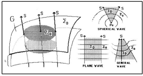
Figure 1: Various geometrical waves G truncated within diffraction-free regions $\Sigma_{D}$ , bound by propagation vectors S ; Within $\Sigma_{O}$ the intensity is zero.

Referring to Fig. 1, a geometrical wave $G(x,y,z,t)$ is truncated according to conditions:

$$G = G\;\;\;\;\text{on}\;\;\Sigma_{D}$$

$$G = 0\;\;\;\;\text{on}\;\;\Sigma_{0}$$ (3)

Where $\Sigma_{D}$ is any limited and well-defined region of space bounded by a ‘wall’ of $S$, and $\Sigma_{O}$ is its complementary region, filling the rest of space outside. Such a wave is, theoretically also a solution because in $\Sigma_{O}$ the wave $G(x,y,z,t)=0$ is also a solution of Eq. 1. This trivial mathematical truth will have great significance when translated to DD physics. In this field, $S$ are straight lines and so within $\Sigma_{D}$ , $G(x,y,z,t)$ constitutes a well-defined geometrical wave. Since energy, by definition, does not cross streamlines, $\Sigma_{D}$ constitutes a ‘flux tube’ ref8 carrying the field’s total energy without any loss whatsoever. $\Sigma_{D}$ is a non-diffracting field. It is important to stress that the border between $\Sigma_{D}$ and $\Sigma_{O}$ does not form a physical barrier to restrain or reflect the waves, such as the walls of a waveguide ref20 nor is there any discontinuity in the medium between $\Sigma_{D}$ and $\Sigma_{O}$ such as a change in the index of refraction: quite simply the amplitude of the waves just drops to zero in certain regions $\Sigma_{O}$ .

Although mathematically possible, such truncated non-diffracting fields do not ordinarily exist in nature ref9 : the moment any attempt is made to truncate an infinite field by placing in its path an opaque screen with an open aperture forming a cross-section of $\Sigma_{D}$ , the field streamlines $S$ automatically swerve behind the screen, slow down near the edge and cause interference effects with regions of zero and maximum intensities, and transform the whole field topologically in a typical diffraction pattern. The field now spreads to fill all of space anew, but now no longer as a geometrical field. Similarly, if the field is emitted from an infinite number of point sources arrayed in an aperture $\Sigma_{D}$ , it diffracts as if a plane wave had passed normally through an open aperture $\Sigma_{D}$ .

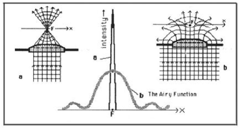
Figure 2: (a) Truncated plane wave super-focused at F, and its spike-like intensity function. (b) An infinite plane wave focused and diffracted an extended Airy intensity function.

Were truncated geometrical fields to exist, they would be very useful indeed. As shown in Fig. 2(a) if a field is passed through a focusing system whose every aperture and field stop is larger than $\Sigma_{D}$ and so does not disturb the edges of the field, it continues to act as a geometrical field and can be theoretically focused to a point with infinite intensity and resolution in imaging systems. Similarly, when the $S$ are parallel, the conceptual flux tube carries a beam of infinite length and uniform cross-section $\Sigma_{D}$ with no loss of intensity. The “diffraction limits” now used as a measure of quality in focusing instruments and beams, and which depend on the wavelength, and inversely on the aperture diameter, would cease to have any significance.

III Geometrical Fields Diffract

In hydrodynamics,

$$\Omega=\text{curl {S}}$$ (4)

is known as the vorticity of the field: it is the measure of how much the field curves around during its flow. When $\Omega=0$ as in Eq. 2, the field is then said to be irrotational ref10 and the vorticity is the same on all of $S$. When such geometrical fields are interrupted or disturbed by a physical obstacle, however, the field acquires vorticity around the edges of the aperture, with $S$ curving into the shadow regions. This is easy to understand by considering sound waves ‘turning’ and being heard behind the corner of a building. Similarly, in hydro- and aerodynamics, obstacles such as the aperture edge can create wakes, vortices and other deviations from geometrical flow ref11 . In wave fields where $\lambda\neq 0$ it is more common to describe these changes as diffraction effects, but in fact I have attempted to show that the two classes of phenomena are closely linked ref5 ; ref6 . An extensive description of the electromagnetic field’s angular momentum, using hydrodynamical concepts has been made by D. Ximing ref12 .

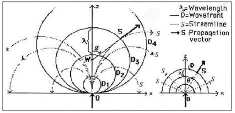
Figure 3: (Left) A dipole or ‘bow-wave’ model of an elementary point field emitted from the origin. (Right) A Huygens-Fresnel wavelet.

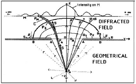
Figure 4: A geometrical field diffracts.

Why do these transformations occur? There is always matter at the edge of a source or an obstacle, where diffraction starts forming. As shown in Fig. 4, the angle $\phi$ which S makes with the normal (the original direction of propagation rotates by $\pi/2$ or more at the edge. Adjoining S follow suit in a domino effect of decreasing $\phi$ until the mainstream $S$ at the center of a symmetrical aperture is reached, where $\phi=0$. This curvature of $S$ around an edge is clearly illustrated by plots of the streamlines and the ellipsoidal wavefronts normal to them, made by Braunbeck and Laukienref13 based on Sommerfeld’s ref14 rigorous solution of the infinite half-plane diffraction problem. This solution also provides another way of visualizing vorticity around the aperture edge: the concept of a cylindrical wave ’emitted’ by the edge, and interfering with the geometrical field to create the diffracted field.

This analysis alternatively gives the diffracted field as an integration of an infinite spectrum of plane waves emitted from the aperture at angles $\phi$ rotating through $\pi$ ref15 . This lends itself naturally to the following physical interpretation: an infinite number of streamlines normal to the aperture make up the original zero-order geometrical field approaching from the $-z$ region. Diffraction bends these $S$ into an infinite number of streamlines each at a different $\phi$, to make up the Fourier orders ($-\pi\leq\phi\leq\pi$) of the field in the $+z$ region ref16 .

Kirchhoff’s theory of diffraction ref17 , although less rigorous than that of Sommerfeld ref14 provides the perfect theoretical framework for demonstrating the transformation of a geometrical field into a diffracted one and then, as shown below, back to a de-diffracted field. A point source $P_{0}$ on the $-z$ axis in Fig. 4 emits a geometrical spherical wave ref18 whose $S$ coincide with the radii centered on $P_{0}$. This wave then passes through an aperture $\overline{AA}$ in an infinite opaque screen and centered on the $x-y$ plane, and spreads throughout the $+z$ portion of space, creating the typical maxima and minima observed on a screen $M$ placed normal to the $z$-axis at some distance from the aperture. Kirchhoff’s method is based on potential theory and is both inaccurate in the vicinity of the edges $A$ and noncommittal on the path the field’s energy takes from $P_{0}$ to $M$. However, the bending of the streamlines into the shadow regions and the transformation of the geometrical wavefront $D_{A}$ into the elliptical wavefronts $D_{1},D_{2},\ldots$ is also quite clear in the rigorous solutions mentioned above ref13 .

A typical flux tube $C$ carries energy from $P_{0}$ to $P_{A}$ in the aperture plane along a straight line. But in the $+z$ region it curves towards the shadow regions behind the obstacle, crossing a typical wavefront $D_{3}$ at $P_{3}$ and creating point $P_{M}$ in the diffraction pattern on $M$. $C$ acts like a channel of a given capacity ref19 , carrying energy from $\overline{P_{0}P_{A}}$ to $P_{M}$ . This idea is confirmed by Helmholtz’ reciprocity (or reversion) theorem ref20 whereby “a point source at $P_{0}$ will produce at $P_{M}$ the same effect as a point source of equal intensity placed at $P_{M}$ will produce at $P_{0}$”. When $P_{0}$ is moved down on the axis to $z=-\infty$ the geometrical field in the $-z$ regions becomes an infinite plane wave arriving normally at $\overline{AA}$. The aspect of Kirchhoff’s integral that is of interest here is that the diffracted field reduces to an integration of Huygens-Fresnel (HF) ref21 wavelets emitted by point sources on $\overline{AA}$. It will be axiomatic to extend this idea to say that a ray from $P_{0}$ reaches the aperture plane at a point $O$ (a source anywhere on the aperture) and is transformed into the ‘exploding’ diffracted pattern of the HF wavelet of Fig. 3 with its inclination factor adjusting the amplitude by $X=(1+\cos\phi)/2$; but this is known to be only an approximation.

Since the precise determination of the wavefronts near the aperture is an essential first step in the implementation of DD theory, an attempt will now be made to examine the wavelet more closely.

IV The Bow Wavelet

A pebble is dropped in a pond and a circular ripple results. But when an atom emits a photon, or when a point element of a field is examined, there is radial momentum but no backward momentum such as in the HF wavelet. Recently Miller ref22 starting out with the wave equation derived a “spatio-temporal dipole” field for the fundamental electromagnetic wavelet. This confirmed my independent intuitive derivation ref23 adapting the model of a bow wave such as that made by a boat ref24 : a stationary atom releases a photon having both radial and foreword velocities $r$ and $f$ and the bow wave or dipole pattern of Fig. 3 emerges. That some such process is at work is suggested by the case of Cerenkov radiation, where a fast-moving electron in glass creates a V-shaped wake of light ref25 . In free space, however, since $r=f=c/2$ the center $W$ of the bow waves’ circular wavefronts $D$, travels up the $+z$ axis at the same rate as the radius $\overline{WP}$ expands, and the V-shaped ‘shock-wave’ now opens up to become a straight line along the $x$-axis. This pattern is also confirmed in the literature, where the streamlines of a dipole ref26 are similar to such circles centered along the $x$-axis. But on this axis, apart from the origin, the field is zero since the contributing wavefronts there would have an infinite radius. The circular streamlines of the bow wavelet provide a natural explanation for the vorticity of the field at the edge of the aperture. In addition the bow wave’s wavelength $\lambda(\phi)$ is $\lambda_{0}$ only in the propagation direction (unlike the HF wavelet which has only amplitude changes with $\phi$. $\lambda(\phi)$ explains the very rapid fluctuations of the diffracted field very near the edge ref13 . This discussion of the primary wavelets of a field is to establish a method to derive the mathematically exact form of the extended wavefronts near the aperture, in order to make DD precise. In section VI experiments will be described that show that the bow wave and the ray that creates it can also have a real physical existence of their own.

V DD: Reversal of the Diffracted Field

It has been long known that electromagnetic fields are time invariant ref27 : any solution $G(x,y,z,+t)$ of Maxwell’s equations will have an equivalent solution $G(x,y,z,-t)$ since replacing $t$ with $-t$, and hence $v$ with $-v$ will lead to the same wave equation Eq. 1. Examples of this are spherical waves and plane waves whose complete solutions show identical waves travelling with opposite velocities $\pm v$, for example the plane wave $G(x,y,z,t)=m(wx+vt)+n(wx-vt)$ ref28 . Time invariance here need not involve any philosophical considerations of the arrow of time, merely that the field retains all its point values when the velocity direction is reversed by rotating all its S by $\pi$. The principle of reversibility along rays has also been derived from Fermat’s principle ref29 .

In optics this principle of reversibility is implicit in any imaging situation where a point object and its image can be interchanged, and in the theory of holography ref30 . With this in mind consider two typical situations where diffraction occurs: First the isolated bow wavelet of Fig. 3. A straight ray is scattered at a point $O$ and then branches into streamlines, creating any of the diffracted wave fronts $D_{1},D_{2},D_{3},\ldots$ Now imagine that a curved mirror shaped as one of the wavefronts say $D_{2}$, is placed to overlap that wavefront exactly. Since all the diffracted streamlines are then normal to the mirror the S vectors are reflected back on themselves, and since amplitude and phase are preserved (phase changes upon reflection will be uniform across $D$) then the field will reverse itself along the same streamlines, and passing point $O$ on the return trip, ends up as a single ray in the $-z$ direction (but without the original source of the ray there) . Alternately, instead of a mirror think that $D_{2}$ now consists of an infinite array of point sources with an identical amplitude function to that of the original diffracted pattern on $D_{2}$. In the $+z$ direction the field will continue to diffract exactly as before. But below $D_{2}$ in the $-z$ direction the sources on $D_{2}$ will recombine to create a reversing ray. The second case is that of an extended field passing through an aperture, for example the diffraction situation of Fig. 5.

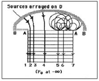
Figure 5: De-diffraction (DD) by reversal of a diffracted wavefront.

Here again any one of the wavefronts $D$ of Fig. 4 can serve as a source for the reverse DD field, or to reflect an already diffracted field. As a result of these procedures, the curved streamlines $1,2,3,\ldots$ of the reversing field emerge from the aperture $\overline{AA}$ normally as a part of a dediffracted truncated geometrical field. If diffraction is to be likened to a topological distortion of an ordinary field, the reverse process can be said to start with a purposely distorted field to produce an ordinary one. It might be argued that the presence of an opaque screen $\overline{BA},\overline{AB}$ reflecting or absorbing portions of the original $-z$ field will necessitate the placement of a similar screen when DD is attempted. Such a screen is not needed for DD however, because the diffracted field immediately touching the screen from the $+z$ side will be negligible or zero; indeed that the field is zero on the screen is one of the boundary conditions in Kirchhoff’s derivation ref17 . Moreover, when the original source is an infinite array of point sources along $\overline{AA}$, no screen $\overline{BA},\overline{AB}$ need be present in the diffracting field, and none will be needed in the reversing field, only the conceptual removal of the original sources on $\overline{AA}$ to allow the DD field to emerge.

Choosing the wavefronts as the source for a DD field insures that the phase is the same there, simplifying the design of the lenses or antennas to be used to create a DD field. However in principle any linear (or surface in the 3D case) array $M$ of sources spanning the diffracted field and mimicking its local phase and amplitude can be used to create the DD field. For example an infinite array of sources having the ring-shaped phase and amplitude pattern of the electric field of the Airy function ref31 , and placed in the focal plane of a lens will cause a reverse DD field to emerge from the lens. This method greatly resembles the zone-plate-type filter described by Toraldo di Francia to achieve superresolution ref2 ; ref3 . Of course, in any practical application, such a filter will have a limited size, and the imitation of the whole diffracted field, and hence of DD, will fail. A more practical filtering DD method would be to wrap a rigid curved holographic film to roughly encircle an aperture, and illuminate both its $z$ sides, in the presence of the aperture, with coherent plane waves. The developed illuminated plate will then recreate the DD field when illuminated from the $+z$ side.

In practice a DD field can be accomplished by any one of five general procedures: 1) An array of sources mimicking the local phase and amplitude values along an entire continuous random cross-section $M$ of the original field. 2) By reflecting a diffracted field normally upon itself. 3) The creation of the wavefronts $D$ by suitably focusing a plane or spherical wave. 4) Holographic methods or 5) A filter illuminated normally by a plane wave (hence the phase is uniform on the filter) having only amplitude changes. Finally, it must be cautioned that when performing DD field calculations, using elementary wavelets, or the Kirchhoff integral, these must be used in the correct orientation. The wavelets always ’point’ from the geometrical rays 5,6,7 of Fig. 5 to the circular diffracted patterns. An integration of bow wavelets on $\overline{AA}$ will give $D$, but integrating wavelets on $D$ will not give the field on $\overline{AA}$ or the DD field in $-z$, since on $D$ the field is already diffracted. A rule of thumb is that the Kirchhoff integral should not be used to evaluate the field of wavefronts such as $D$, whose normals S rotate rapidly through $\pi/2$ at the aperture edge.

VI De-Diffraction Experiments

Simple experiments to prove the DD methods outlined in this paper were performed as follows, but a more sophisticated experimental verification of DD using electromagnetic radiation is still needed.

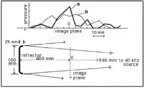
Figure 6: Ultrasound wave field measured after reflection from (a) DD plane reflector, and (b) From a plane reflector of the same size.

DD OF ULTRASOUND WAVES: The field of a 40 kHz ultrasound source as reflected from a plane antenna and one with curved edges were compared as in Fig. 6. The curved edges, roughly approximating the curvature of a DD wavefront, concentrated the field appreciably.

Figure 7: Photographs of waves emitted in a ripple tank from (a) A vibrating plate reflector three wavelengths wide, and (b) From its DD equivalent.

WATER RIPPLES: Water ripple experiments are shown in Fig. 7: a) a vibrating flat plate produced ripples of a wavelength one third its width spreading out in the typical oval diffracted wavefronts (b) roughly curving the edges through a quarter-circular arc of about one $\lambda$ radius produced a dramatic concentration of the waves mainly in the forward direction. Note the absence of waves from either side of the axis in (b): the waves in the bottom right of (b) are spurious, since they are emitted from the back of the plate.

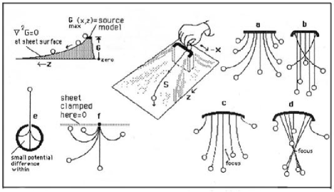
Figure 8: Diagrams of gravity potential field experiments. The path taken by a marble rolling down a flexible sheet stretched over elevated forms, simulates the streamlines S of (a) A diffracted plane wave, (b) DD plane wave, (c) Diffracted focused wave, (d) Focused wave, (e) DD (reversed) bow wave and (f) Bow wave.

GRAVITATIONAL MODEL. It is known that a thin flexible rubber sheet stretched over a solid two dimensional horizontal model of a certain function $G(x,y)$ satisfies Laplace’s equation of $G$: Freezing a wave in time reduces the right hand term of Eq. 1 to zero, and the wave equation becomes $\nabla^{2}G=0$. The surface of the sheet represents both the gravitational and electrostatic potentials of this Laplacian ref32 . For our purposes, the potential of the fields we are studying was represented by a flat model $G(x,z)$ of the wavefront in question. The model was lifted a distance $G_{max}$ representing the initial potential of the wave and the sheet stretched over the model as in Fig. 8.

The gravity-wave-potential equivalence mentioned above (and which might not be coincidental, as discussed below) allows a study of the streamlines $S$ of the field since they will be the path taken by a marble rolling down the sheet’s surface. The equipotential horizontal contours of the sheet’s surface ($G_{1},G_{2},G_{3},\ldots$ the ‘elevation’) are then the wavefronts. $G_{max}$ is proportional to the energy of the source (inversely proportional to the wavelength) and it is interesting to see how increasing the height of the model reduces the diffraction spreading, according to theory. This method though not too quantitatively exact if the membrane slope is larger than around $18^{\circ}$, gives an excellent idea of the physical situation. As shown in the streamline sketches of Fig. 8, such a gravitational model was used to prove that DD proceeds exactly as theoretically predicted for a diffracted and de-diffracted plane (a,b) and focused (c,d) waves. The concentration of the streamlines at a single point-focus in case (d) was a dramatic demonstration of superresolution. The bow wavelet pattern both in the emission (f) and the DD reversing (a) modes (a lone ray) was also verified. In the case of the point source (f) the sheet was also clamped down ($G=0$) along $x$ except for a spike at the origin, because the source was assumed to be located on a flat non-conducting plane. The paths of the rolling marble in (f) were very similar to the streamlines of the bow-wavelet $S$ of Fig. 3.

VII Practical Applications of DD

The cancellation of diffraction improves the performance of a wide range of instruments in many fields. These can be roughly categorized according to whether the truncated field is to be focused or allowed to propagate as a beam. And also according to the type of field such as optical, microwave, acoustic etc. Examples are too numerous to list, but focused field applications include cameras, telescopes (optical and radio) microscopes (optical and electron), imaging radar, and sonar. Beam applications include lasers and tele-communication parabolic antennas. In the case of imaging radar, for example, DD methods ref5 ; ref6 , applied through refocusing the field by reshaping the antenna by curving its rim, will allow fine resolution even with a large wavelength and a small antenna, since a truncated geometrical field can be focused to a point regardless of the field’s wavelength or the aperture size. An optical laser passing through a DD lens with curved edges pointed towards the moon should proceed with no divergence (apart from atmospheric degradation), reaching its target with its original profile relatively intact. Normally diffraction would spread a 10 cm. diameter laser beam to some two kilometers in diameter by the time it arrives there.

VIII Diffraction, Quantum and relativistic Fields

Diffraction has been cited by Heisenberg himself (33) as an example of uncertainty relations. The product of a photon’s momentum and position cannot be less than Planck’s constant $h$. The question now arises: are uncertainty and hence quantum effects cancelled together with the cancellation of diffraction? The inescapable conclusion is that they are, since both momentum and position would be uniquely known in a DD geometrical field. The vectors S of a plane DD field all point in the same direction, and the position is always known within $\Sigma_{D}$ especially in the case of a single ray. In the bow wavelet itself the change from a ray (position and momentum precisely known) to the spread-out diffracted wavelet, with its momentum vectors fanning out at all angles is a model of this transformation from a classical field (the ray) to a quantum field (the fan) and vice versa. Are elementary particles emitting bow wavelets the physical machinery ref34 behind quantum effects? Two particles $P_{1}$ and $P_{2}$ emit bow waves which meet at a random angle $(\phi_{1}-\phi_{2})$ and the resulting interference pattern is taken for that of quantum probability functions. Here then is the physical ‘cause’ of quantum effects: it is the variable energy content transmitted by streamlines or flux tubes from $P_{1}$ and $P_{2}$ to a nearby point $T$, which can be considered as the probability amplitudes ref35 $<P_{1}|T>$ and $<T|P_{2}>$.

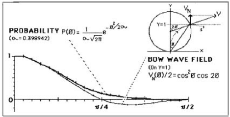
Figure 9: Bow wave and probability functions.

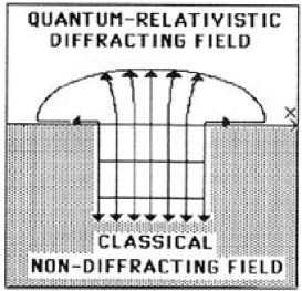
Figure 10: The transformation of a classical field through diffraction into a field with quantum and general-relativistic characteristics.

Fig. 9 shows the similarity between a Gaussian probability function ref36 and the normal of the electric field of a bow wavelet around the propagation axis. Discussions following Toraldo di Francia’s paper on super-resolving filters ref2 also raised the question of quantum uncertainty in diffracted fields, and included this remark: “the only correct quantum electrodynamical version of Heisenberg’s principle imposes no relevant restrictions on resolving power to begin with.” One can speculate even further. The emerging circular streamlines of the bow wavelet first propagate foreword and then ‘fall’ towards the source like a fountain, as if attracted towards the origin. Can the streamlines and equipotential surfaces of the primary wavelet then be interpreted as curved Gaussian coordinates (S being the geodesics ref37 ) of a relativistic gravitational distortion of the field surrounding the atom emitting the photons? This would be a miniature version of Einstein’s results concerning the bending of light in the vicinity of a massive star ref38 . Considering the proportionally smaller atomic masses and distances involved, this might not be too improbable. The distortion of space in the vicinity of an obstacle can be easily observed by moving a pinhole or slit with an aperture of about 1 mm in front of the eye. The aperture seems to act like a concave lens distorting the view, according to the divergence of the diffracted streamlines ref39 . Thomas Young had also combined gravitational and optical concepts to explain diffraction. He hypothesized that the rays refract through a lens-like, increasingly dense ethereal fluid surrounding the obstacle, “attracted to particles of gross matter” ref40 . In view of the preceding analysis, the intriguing possibility exists that sub-atomic bow waves propagated into space can be considered the source of a unified field combining quantum, relativistic-gravitational and electromagnetic effects. In that case field reversal methods such as DD can provide a way to transform quantum-relativistic fields in space into classical ones, and vice versa, as in Fig. 10. But all such speculation must first await acceptance and further experimental proof of DD.

IX Summary and Conclusion

A method was presented, starting from the wave equation, and a truncated version of a geometrical field, and the principle of reversal of wave fields, whereby de-diffracted geometrical wave fields can be created. To clarify the process, the conversion of a ray into the diffracted primary wavelet and back to a ray was studied as a model of such a DD transformation. DD methods allow superresolution in imaging instruments and for infinite beams with no divergence. The simple experiments performed to prove DD could be repeated and refined. Rigorous computer simulation of the field can find the precise waves D for a given device and thus provide the exact design of a DD lens, antenna or other instrument. The similarity of the field equations of flow fields, gravity and electrostatics suggest that methods equivalent to DD might also be used to modify those fields too. For example a boomerang-shaped object would have its gravitational field lines ’focused’ on the concave side. Finally it was speculated whether diffraction could be just one manifestation of a united quantum-relativistic field surrounding an atom, and conversely whether DD means that it is possible to create classical-field regions of space free from such effects.

- (1) S. Schelkunoff, Bell Syst. Techn.Journ. 22, 80 (1943).
- (2) G. Toraldo Di Francia, Nouvo Cimento Suppl. IX, 391-438 (1952).
- (3) I. Cox, C. Sheppard, and T. Wilson, J. Opt. Soc. Am. 72, 1287-1291 (1982).
- (4) J. Durnin, J. Opt. Soc. Am. A 4, 651-654 (1987).
- (5) V. Tamari, Optoelectronics-Devices and Tech. 2, 59-81 (1987).
- (6) V. Tamari, U.S. Patents No. 5,148,315, Sept. 15, 1992 and No. 5,392,155, Feb.21, 1995.
- (7) M. Born and E Wolf, Principles of Optics, 6th.ed. Pergamon, 109-132, (1980).
- (8) W. Hayt, Jr., Engineering Electronics, 3d. Ed., McGraw-Hill, 174, (1974).
- (9) But occasionally, a truncated ripple pattern, similar to the experimental one in Figure 7(b) has been observed in a stream, ’focused’ by a chance arrangement of pebbles and leaves. Also a primitive attempt to create DD sound waves is when a person instinctively cups his or her hands around the mouth to concentrate the emerging waves when shouting to a distant hearer.
- (10) R. Feynman, R Leighton, and M. Sands, The Feynman Lectures on Physics II 40-5 Addison-Wesley (1965).
- (11) S. Goldstein, ed., Modern Developments in Fluid Dynamics, Dover, 61-65 (1965).
- (12) D. Ximing, Laser & Particle Beams 10, 117-134 (1992).
- (13) W. Braunbek and G. Laukien, Optik 9, 174-179 (1952); see also M. Born and E. Wolf, Principles of Optics, op.cit., 575-77.
- (14) Sommerfeld, Math.Ann. 47, 317 (1896); see also M. Born and E. Wolf, Principles of Optics, op.cit., 556-77.
- (15) E. T. Whittaker and G. N. Watson, A Course of Modern Analysis, Camb. Univ., 397 (1927); see also M. Born and E. Wolf, Principles of Optics, op.cit.,562.
- (16) J. Goodman, Introduction to Fourier Optics, McGraw-Hill, (1968).
- (17) G. Kirchhoff, Ann. Physik. 18,663 (1883); see also M. Born and E. Wolf, Principles of Optics, op.cit., 375-382.
- (18) M. Born and E. Wolf, Principles of Optics, op.cit., 15.
- (19) I. Cox and C. Sheppard, J. Opt. Soc. Am. A 3, 1152-1158 (1986).
- (20) L. H. Huxley , The Principles and Practice of Waveguides, Camb. Univ. Press, 7.17, (1947); see also M. Born and E. Wolf, Principles of Optics, op. cit.,381,584.
- (21) C. Huygens, Traite de la Lumiere, Leyden (1690); see also M. Born and E. Wolf, Principles of Optics, op.cit., 370.
- (22) D.A.B. Miller, Optics Lett. 16, 1370-1372 (1991).
- (23) V. Tamari ”Bow Wave Geometry” postdeadline paper, ”Huygens’ Principle 1690-1990” Conference. Scheveningen, The Netherlands (1990).
- (24) F. Crawford, Am. J. Phys. 52, 782-785, (1984).
- (25) N. Feather, Vibrations and Waves, Pelican, 252-3 (1961).
- (26) W. Hayt, Jr., Engineering Electronics, op. cit., 116.
- (27) J. Coveney and R. Highfield, The Arrow of Time, W.H. Allen, 58-62 (1990).
- (28) M. Born and E. Wolf, Principles of Optics, op. cit., 14,15.
- (29) E. Hecht and A. Zajac, Optics, Addison-Wesley, 70 (1974).
- (30) D. Gabor, Nature 161, 777 (1948).
- (31) G. Airy, Trans. Camb. Phil. Soc. 5, 283 (1835); see also M. Born and E. Wolf, Principles of Optics, op.cit., 396.
- (32) W. Hayt, Jr., Engineering Electronics, op. cit., 181.
- (33) W. Heisenberg, The Physical Principles of the Quantum Theory, U. of Chicago Press (1930).
- (34) R. Feynman, R. Leighton, and M. Sands, The Feynman Lectures on Physics III, op. cit., 1-10; Dr. Feynman said quantum effects in the double slit experiment cannot be explained by any ’machinery’ within the electron.
- (35) R. Feynman, R. Leighton , and M. Sands, The Feynman Lectures on Physics III, op. cit., 3-2.
- (36) R. Feynman, R. Leighton , and M. Sands, The Feynman Lectures on Physics I, op. cit., 6-9.
- (37) W. Rindler, Essential Relativity, Springer-Verlag, 182 (1977).
- (38) A. Einstein, Relativity, The Special and General Theory, Bonanza, 126-132 (1961).
- (39) Pinholes and slits have been routinely used by optometrists in place of lenses to test for myopia and astigmatism. See H. Kumagai (ed.) Lectures on Eyeglasses, Vol.II, Koryu Shuppansha, 33 (1985) (In Japanese); Striking parallax effects of nearby objects can also be seen through these devices.
- (40) T. Young, Philos. Trans. R. Soc. London 92, facing p.48 (1802); see also G. Cantor, Am. J. Phys. 52, 305-308 (1984).