Importance of direct and indirect triggered seismicity in the ETAS model of seismicity

Abstract

Using the simple ETAS branching model of seismicity, which assumes that each earthquake can trigger other earthquakes, we quantify the role played by the cascade of triggered seismicity in controlling the rate of aftershock decay as well as the overall level of seismicity in the presence of a constant external seismicity source. We show that, in this model, the fraction of earthquakes in the population that are aftershocks is equal to the fraction of aftershocks that are indirectly triggered and is given by the average number of triggered events per earthquake. Previous observations that a significant fraction of earthquakes are triggered earthquakes therefore imply that most aftershocks are indirectly triggered by the mainshock.

HELMSTETTER and SORNETTE Importance of triggered seismicity Agnès Helmstetter, Institute of Geophysics and Planetary Physics, University of California, Los Angeles, California. (e-mail: helmstet@moho.ess.ucla.edu) Didier Sornette, Department of Earth and Space Sciences and Institute of Geophysics and Planetary Physics, University of California, Los Angeles, California and Laboratoire de Physique de la Matière Condensée, CNRS UMR 6622 and Université de Nice-Sophia Antipolis, Parc Valrose, 06108 Nice, France (e-mail: sornette@moho.ess.ucla.edu)

1 Introduction

There is a growing awareness and an intense research activity based on the fact that a significant fraction of earthquakes are events triggered (in part) by preceding events. In addition, a significant part of triggered events may be indirectly triggered by a previous event through a cascade process. What is then the relative role of earthquake interactions and triggering compared with the underlying tectonic driving forces? Is there a way to distinguish triggered earthquakes from untriggered ones or to estimate the proportion of directly or indirectly triggered earthquakes? Here, we use the Epidemic-Type Aftershock Sequence (ETAS) model to offer a quantification of earthquake interactions. This model is based on the two best established empirical laws of seismicity, the Gutenberg-Richter and the Omori law. The ETAS model has been used in many studies to describe or predict the spatio-temporal distribution of seismicity and reproduces many properties of real seismicity (see [Ogata, 1999] and [Helmstetter and Sornette, 2002] for reviews). The ETAS model assumes that the seismicity results from the sum of an external constant loading and from earthquakes triggered by these sources in direct lineage or through a cascade of generations. From this definition (see below), it is clear that the ETAS model is not only a model of aftershock sequences, as the acronym ETAS would make one to believe, but describes the global seismicity including background and interacting triggered seismicity. We use this model to quantify (a) the fraction of triggered events relative to the sources and (b) the fraction of indirectly triggered events with respect to the total triggered seismicity.

Question (a) has been previously visited in order to provide unambiguous definitions of aftershocks and to decluster seismic catalogs. Several alternative algorithms for the definition of aftershocks have been proposed [see Molchan and Dmitrieva, 1992 for a review]. Gardner and Knopoff [1974] and Knopoff [2000] used a windowing method and found that 2/3 of the events in the catalog of Southern California are aftershocks. Reasenberg [1985] analyzed the central California catalog and found that 48% of the events belong to a seismic cluster. Davis and Frohlich [1991] used the ISC catalog and found that 30% of earthquakes belong to a cluster, of which 76% are aftershocks and 24% are foreshocks. Kagan [1991] estimated the ratio of dependent events in various catalogs (California and worldwide) using an inversion by the maximum likelihood method of the ETAS model. The proportion of dependent earthquakes of the first generation that he estimated displays huge fluctuations from 0.1% for deep events to 90%, but is often close to 20%.

With respect to question (b), it has long been suggested that aftershocks may produce their own aftershocks, commonly known as secondary or indirect aftershocks. The observation of large and sudden changes of the seismicity rate after a mainshock [e.g. Correig et al., 1997] and the existence of strong spatio-temporal clustering of aftershocks shows that a significant proportion of aftershocks may be triggered indirectly by the mainshock, that is, they may be aftershocks of aftershocks triggered by the mainshock [Felzer et al., 2003]. For instance in Southern California, the $M=6.5$ Big-Bear earthquake occurred a few hours following the Landers $M=7.3$ event and has clearly triggered its own aftershock sequence. While each aftershock induces a negligible stress change by comparison to the mainshock, all aftershocks when taken together can significantly alter the stress field induced by the mainshock, so that most aftershocks at large times after the mainshock are triggered by previous aftershocks of the mainshock. Felzer et al. [2002] estimated the rate of indirect aftershocks, from a comparison of the Landers aftershock sequence with numerical simulations of the ETAS model. They found that about 85% of the aftershocks of the Landers event were indirect aftershocks. This implies that the 1999 $M_{W}=7.1$ Hector Mine earthquake was triggered, not by the 1992 $M_{W}=7.3$ Landers earthquake itself [Felzer et al., 2002], but more likely by some of its direct and indirect aftershocks. Felzer et al. [2003] further analyzed the temporal evolution of the proportion of secondary aftershocks. They found that, after a few days or weeks following a mainshock depending on mainshock magnitude, most aftershocks are secondary aftershocks. We now recall the formulation of the ETAS model and its main results on the importance of triggered seismicity.

2 The ETAS model of triggered seismicity

The present parametric form of the ETAS model used in this paper was formulated by Ogata [1988]. We refer to [Ogata, 1999; Helmstetter and Sornette, 2002] for reviews on the ETAS model and for a discussion of the model parameters. The ETAS model assumes that a given event of magnitude $m_{i}\geq m_{0}$ occurring at time $t_{i}$ triggers other events in the time interval between $t$ and $t+dt$ at the rate

$$\phi_{m_{i}}(t-t_{i})=\rho(m_{i})~{}\Phi(t-t_{i})~{}.$$ (1)

$\Phi(t)$ is the direct Omori law normalized to $1$

$$\Phi(t)={\theta~{}c^{\theta}\over(t+c)^{1+\theta}},$$ (2)

where $c$ is a regularizing time scale that ensures that the seismicity rate remains finite close to the mainshock. The average number of aftershocks triggered directly by an event of magnitude $m$ is

$$\rho(m)=k~{}10^{\alpha(m-m_{0})}~{},$$ (3)

where $m_{0}$ is a lower bound magnitude below which no daughter is triggered. The model is complemented by assuming that each earthquake has a magnitude independently chosen according to the density distribution $P(m)$. The magnitude distribution is usually taken equal to the Gutenberg-Richter law $P(m)\sim 10^{-b(m-m_{0})}$ with eventually a cut-off for large magnitudes. The model can also be extended to include the spatial distribution of seismicity [Ogata 1999]. The key parameter of the ETAS model (1) is the average number (or “branching ratio”) $n$ of directly triggered earthquakes per mother-event. This average is performed over time and over all possible mother magnitudes. The branching ratio has a finite value for $\theta>0$ equal to

$$n\equiv\int\limits_{0}^{\infty}dt\int\limits_{m_{0}}^{\infty}~{}P(m)~{}\rho(m)~{}\Phi(t)~{}dm~{}.$$ (4)

The normal regime corresponds to the subcritical case $n<1$ for which the seismicity rate decays after a mainshock to a constant level (in the case of a steady-state source). Note that the realized number of aftershocks for a given earthquake is not $n$ but depends on its magnitude, according to the function $\rho(m)$ given by (3).

The total seismicity rate (or intensity) $\lambda(t)$ at time $t$ is given by the sum of the “external” source $s(t)$ and of the aftershocks triggered by all previous events

$$\lambda(t)=s(t)+\sum_{i|t_{i}\leq t}\phi_{m_{i}}(t-t_{i})~{}.$$ (5)

This external source $s(t)$ acts as an external driving force ensuring that the seismicity does not vanish.

Taking the ensemble average of (5) over many possible realizations of the seismicity, we obtain the following equation for the first moment or statistical average $N(t)$ of $\lambda(t)$ [Sornette and Sornette, 1999; Helmstetter and Sornette, 2002]

$$N(t)=s(t)+n\int\limits_{-\infty}^{t}~{}\Phi(t-\tau)~{}N(\tau)~{}d\tau.$$ (6)

The average seismicity rate is the solution of this self-consistent integral equation, which embodies the fact that each event may start a sequence of events, which can themselves trigger secondary events, and so on.

The global rate of aftershocks including indirect aftershocks triggered by a mainshock of magnitude $M$ occurring at $t=0$ is given by $\rho(M)K(t)/n$, where the renormalized Omori law $K(t)$ is obtained as a solution of (6) with the general source term $s(t)$ replaced by the Dirac function $\delta(t)$. The solution for $K(t)$ is given in [Helmstetter and Sornette, 2002] and is illustrated in Figure 1. The effect of the cascade of direct, secondary, and later-generation aftershocks is to renormalize the bare Omori law $\Phi(t)\sim 1/t^{1+\theta}$ into $K(t)\sim 1/t^{1-\theta}$ at early times $t\ll t^{*}$ where $t^{*}\approx c|1-n|^{-1/\theta}~{}$. The characteristic time $t^{*}$ is infinite for $n=1$ and becomes very small for $n\ll 1$. Figure 1 also shows the rates $N_{i}(t)$ of aftershocks of generation $i$, for $i=1$ to $20$. Taking an ensemble average, we predict $N_{1}(t)=\rho(M)\Phi(t)$, $N_{2}(t)=\int_{0}^{t}n\Phi(t-\tau)~{}\rho(M)~{}\Phi(\tau)d\tau$, and more generally

$$N_{i}(t)=n\int_{0}^{t}\Phi(t-\tau)~{}N_{i-1}(\tau)~{}d\tau~{},$$ (7)

such that the total seismicity rate is reconstructed as the sum $N(t)=\sum_{i=1}^{\infty}N_{i}(t)$. Figure 1 illustrates clearly the role and importance of the successive generation of indirect aftershocks in the construction of the global observable seismicity.

In real data, it is impossible to distinguish unambiguously aftershocks from background seismicity, or direct aftershocks from indirect aftershocks. The distinction is only probabilistic. Each event results in part from the external loading and in part from the effect of all previous earthquakes. Knowing the parameters of the model, we can however estimate the probability that each event results from the external source or is an aftershock of a previous earthquake [Kagan, 1991]. In the sequel, we estimate the ratio of triggered seismicity over total seismicity in section 3 and the proportion of secondary aftershocks over total aftershocks in section 4, and we show that these two quantities are equal to the branching ratio $n$.

3 Proportion of aftershocks

Let us consider the situation in which $s(t)$ corresponds to a constant Poisson source process with intensity $\mu$, representing the effect of the external loading. Then, the observed seismicity results both from this constant source rate and from the direct and indirect aftershocks triggered by this constant external loading. In the regime $n<1$, the global seismicity is stationary, with large fluctuations following large earthquakes due to the triggered aftershock sequences. The rate of aftershocks $r_{0}$ triggered directly by the tectonic source $\mu$ is on average $r_{1}=\mu n$ because each single event triggers on average $n$ events, when averaging over all magnitudes. The rate of second generation aftershocks, triggered by aftershocks of the tectonic source, is $r_{2}=nr_{1}=\mu n^{2}$. At the $i^{th}$ generation, the rate of aftershocks triggered indirectly by the tectonic source $\mu$ is given by $r_{i}=\mu n^{i}$. Summing over all generations, the global rate $R_{aft}$ of direct and indirect aftershocks of the constant external source in the sub-critical regime $n<1$ is given by

$$R_{aft.}=\sum_{i=1}^{i=\infty}r_{i}=\mu\sum_{i=1}^{i=\infty}n^{i}={\mu n\over 1-n}~{}.$$ (8)

The global seismicity rate $R$ is given by the sum of the external loading $\mu$ and of the rate of aftershocks $R_{aft.}$:

$$R=\mu+R_{aft.}=\mu+{\mu n\over 1-n}={\mu\over 1-n}~{}.$$ (9)

The result (9) shows that the effect of the cascade of aftershocks of aftershocks and so on is to renormalize the external constant source $\mu$ to a higher level $R$ that increases as $n$ is close to the critical value 1, as illustrated in Figure (2). This result is well-known in the branching process literature [Harris, 1963] and has also been derived by Kagan [1991] for the slightly modified version of the ETAS model using $c=0$ and replacing it by an abrupt cut-off at early times.

The proportion of aftershocks (of any generation) is thus equal to ${R_{aft.}/R}=n$. This expression shows that the average branching ratio $n$ can be directly observed from a suitable analysis of seismicity catalogs. Indeed, clustering algorithms for detecting and counting aftershocks provide a direct estimation and in general a lower bound of $n$ because most triggered events cannot be distinguished from the background seismicity. Note that the result (9) can also be derived directly from the master equation (6) by inserting $s(t)=\mu$ in (6) and taking the expectation of $N(t)$.

4 Proportion of indirect aftershocks

There is another interpretation for $n$ as well as an additional empirical tool to estimate it. We calculate the total number of aftershocks $n_{t}$ triggered by a mainshock of magnitude $M$, including all the generations of direct and indirect aftershocks, as follows. The number of direct aftershocks is given by $n_{1}=\rho(M)$ using the definition (1). The average number of second generation aftershocks $n_{2}$ is given by the product of $n_{1}$ with the average number of aftershocks per earthquake defined by $n$. Therefore $n_{2}=\rho(M)n$. The number of third generation aftershocks of the mainshock is $n_{3}=\rho(M)n^{2}$. The number of aftershocks for the $i^{th}$ generation is $n_{i}=\rho(M)n^{i-1}$. The total number of aftershocks triggered by a mainshock of magnitude $M$ is thus given by

$$S=\sum_{i=1}^{\infty}n_{i}=\rho(M)\sum_{i=0}^{\infty}n^{i}={\rho(M)\over 1-n}~{}.$$ (10)

For $n\ll 1$, $S\approx\rho(M)$, i.e., most aftershocks are directly triggered by the mainshock. For $n\approx 1$, $S\gg\rho(M)$, i.e., most aftershocks are indirect aftershocks of the mainshock. The proportion of indirect aftershocks is given by

$${S-n_{1}\over S}={{\rho(M)\over 1-n}-\rho(M)\over{\rho(M)\over 1-n}}=n~{}.$$ (11)

This result (11) shows the fraction among all aftershocks of the aftershocks triggered indirectly by the mainshock is given by the average branching ratio $n$, independently of the mainshock magnitude $M$. We can also derive the result (11) from the master equation (6). Inserting $s(t)=\delta(t)\rho(M)$ in (6) and taking the integral of (6) gives after some manipulation the global number of direct and indirect aftershocks

$$S=\int\limits_{0}^{\infty}N(t)dt=\rho(M)+n\int\limits_{0}^{\infty}~{}N(\tau)~{}d\tau=\rho(M)+n~{}S~{},$$

which recovers expression (10) for $S$.

The branching ratio $n$ gives the proportion of indirect aftershocks averaged over the whole aftershock sequence. It is different from the instantaneous proportion of indirect aftershocks $\nu(t)$ that is defined by

$$\nu(t)={K(t)-\Phi(t)\over K(t)}~{},$$ (12)

which can be computed analytically using the expression of $K(t)$ given by Helmstetter and Sornette [2002]. The instantaneous proportion of indirect aftershocks increases from 0 for very small times $t\ll c$ (all aftershocks are triggered directly by the mainshock) to a maximum value smaller than one at large times $t\gg t^{*}$ given by

$$\nu_{\infty}=\lim_{t\to\infty}\nu(t)=1-(1-n)^{2}~{}{\theta~{}\Gamma(\theta)\over\Gamma(1-\theta)}~{}.$$ (13)

The temporal evolution of $\nu(t)$ given by (12) is illustrated in the inset of Figure 1.

5 Conclusion

We have shown that, in the ETAS model, the proportion of earthquakes that are triggered is equal to the proportion of aftershocks that are indirect, and is given by the branching ratio. Previous observations that a significant fraction of earthquakes are triggered earthquakes therefore imply that most aftershocks are indirectly triggered by the mainshock. The importance of indirect aftershocks casts doubts on the relevance of prediction of aftershocks rate based on the calculation of the Coulomb stress change induced by the mainshock only, neglecting the stress changes induced by aftershocks [Stein, 1999]. It also opens the road for improved methods of seismicity forecasts [Felzer et al., 2003].

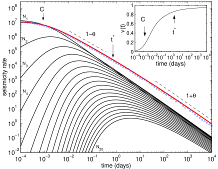
Figure 1: A realization of the ETAS model showing the realized seismicity rate $\lambda(t)$ (circles) following a $M=7$ mainshock obtained by averaging over 1000 simulations with $n=0.8$, $\alpha=0.8$, $b=1$, $\theta=0.2$, $m_{0}=0$, $c=0.001$ day, and the average renormalized propagator $K(t)$ (solid gray line). The bell-shaped curves show the seismicity rates $N_{i}(t)$ of aftershocks of generation $i$ estimated from equation (7), for $i=1$ to $20$ from top to bottom. The inset gives the proportion of indirect aftershocks $\nu(t)$ evaluated by (12). After 15 minutes, most aftershocks are triggered indirectly by the mainshock. At large times $t\gg t^{*}$, the proportion of indirect aftershocks goes to an asymptotic value of 0.97.

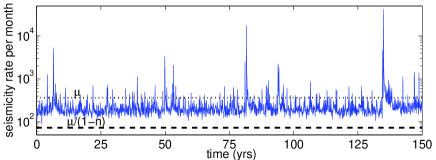
Figure 2: Rate of seismic activity for a synthetic catalog generated using the ETAS model with parameters $\mu=0.1$ source events per day, $c=0.001$ day, $n=0.8$, $\theta=0.2$, $b=1$ and $\alpha=0.8$. The average seismicity rate is close to the expected value $\mu^{*}=\mu/(n-1)$ predicted by (9) (dotted line) and is always significantly larger than the constant external rate $\mu$ (dashed line). 78% of earthquakes are aftershocks, among which 79% are indirect aftershocks, in good agreement with the predictions (9) and (11).

- [1] Correig, A.M., M. Urquizú and J. Vila, Aftershock series of event February 18, 1996: An interpretation in terms of self-organized criticality, J. Geophys. Res., 102, 27,407-27,420, 1997.
- [2] Davis, S. D. and C. Frohlich, Single-link cluster analysis of earthquake aftershocks: decay laws and regional variations, J. Geophys. Res., 96, 6335-6350, 1991.
- [3] Felzer, K. R., T. W. Becker, R. E. Abercrombie, G. Ekström and J. R. Rice, Triggering of the 1999 Hector Mine earthquake by aftershocks of the 1992 Landers earthquake, J. Geophys. Res., 107, doi:10.1029/2001JB000911, 2002.
- [4] Felzer, K. R., R. E. Abercrombie and G. Ekström, Secondary aftershocks and their importance for aftershock forecasting, submitted to Bull. Seism. Soc. Am., 2003.
- [5] Gardner, J. K. and L. Knopoff, Is the sequence of earthquakes in Southern California, with aftershocks removed, Poissonian?, Bull. Seismol. Soc. Amer., 64, 1363-1367, 1974.
- [6] Harris, T. E., The theory of branching processes, Springer, Berlin, 1963.
- [7] Helmstetter, A. and D. Sornette, Sub-critical and Super-critical Regimes in Epidemic Models of Earthquake Aftershocks, J. Geophys. Res., 107, 2237, 10.1029/2001JB001580, 2002.
- [8] Kagan, Y. Y., Likelihood analysis of earthquake catalogues, Geophys. J. Int., 106, 135-148, 1991.
- [9] Knopoff, L., The magnitude distribution of declustered earthquakes in Southern California, Proc. Natl. Acad. Sci. USA, 97, 11880-11884, 2000.
- [10] Molchan, G. M. and O. E. Dmitrieva, Aftershock identification – Methods and new approaches, Geophys. J. Int., 109, 501-516, 1992.
- [11] Ogata, Y., Statistical models for earthquake occurrence and residual analysis for point processes, J. Am. Stat. Assoc., 83, 9-27, 1988.
- [12] Ogata, Y., Seismicity analysis through point-process modeling: a review, Pure Appl. Geophys., 155, 471-507, 1999.
- [13] Reasenberg, P., Second-order moment of central California seismicity, 1969-82, J. Geophys. Res., 90, 5479-5495, 1985.
- [14] Stein, R. S., The role of stress transfer in earthquake occurrence, Nature, 402, 605-609, 1999.
- [15] Sornette, A. and D. Sornette, Renormalization of earthquake aftershocks, Geophys. Res. Lett., 26, 1981-1984, 1999.