Lattice Boltzmann Study of Velocity Behaviour in Binary Mixtures Under Shear

Abstract

We apply lattice Boltzmann methods to study the relaxation of the velocity profile in binary fluids under shear during spinodal decomposition. In simple fluids, when a shear flow is applied on the boundaries of the system, the time required to obtain a triangular profile is inversely proportional to the viscosity and proportional to the square of the size of the system. We find that the same behaviour also occurs for binary mixtures, for any component ratio in the mixture and independently from the time when shear flow is switched on during phase separation.

I Introduction

Recently, the dynamical behaviour of complex fluid and binary mixtures under the action of applied flows has been investigated in many theoretical and experimental works [1]. In phase separating binary mixtures the morphology and the growth properties of the domains of the two components are greatly affected by the presence of a flow[2]. This flow is generally imposed from the boundaries onto the system and takes some time to reach its steady value. If this time is comparable with other typical time-scales in the system, transient effects have to be carefully considered. For example, in the case of an oscillating shear flow, the ratio between the period of the applied flow and the relaxation time of a triangular steady shear profile is relevant for the effectiveness of the flow on the bulk of the system. In spinodal decomposition, if that ratio is small, the growth remains mainly isotropic and elongated domains can be observed only in the boundary layers [3].

The estimation of relaxation times of applied flows is generally based on analogies with simple fluids. However, a careful checking of the laws valid for simple fluids in cases when mesoscopic structures are present in the system - e.g. interfaces between domains in spinodal decomposition, cannot be found in literature. In this paper we evaluate numerically the relaxational properties of a triangular shear flow applied on phase separating binary mixtures. At a certain time during phase separation the top and the bottom boundaries of our system start to move with velocities $w$ and $-w$ respectively and after a while a triangular profile will appear. We study the evolution of the velocity field in terms of the viscosity and of the size of the system and find that the results for a simple fluid also hold in the case of binary mixtures with interfaces inside.

We simulate the binary mixture system by applying lattice Boltzmann methods which allow to mimic the behaviour of a system described by Navier-Stokes and convection-diffusion equations. The lattice Boltzmann algorithm is based on a collision step and a propagation step occurring on time $\Delta t$. Only a finite sets of local velocities are allowed. In particular we use a scheme based on a free-energy approach which has the advantage that the equilibrium thermodynamics of the system is “a priori” known. The role of the simulation time step $\Delta t$ will be also considered. With fast relaxing velocity profiles, the usual choice $\Delta t=1$ is not appropriate for obtaining smoothly relaxing profiles and smaller $\Delta t$ have to be considered.

In the next section we briefly describe the methods used in the simulations; section III contains our results and section IV some conclusions.

II The model

We consider a two-dimensional binary fluid with components A and B of number density $\rho_{A}$ and $\rho_{B}$, respectively. Such a system can be modeled by the following free energy functional,

$$F=\int d{\bf r}[\frac{1}{3}\rho\ln\rho+\frac{a}{2}\varphi^{2}+\frac{b}{4}\varphi^{4}+\frac{\kappa}{2}(\nabla\varphi)^{2}]\text{, }$$ (1)

where $\rho=\rho_{A}+\rho_{B}$ is the local total density and $\varphi=\rho_{A}-\rho_{B}$ is the local density difference and the order parameter of the system; the term in $\rho$ gives rise to a positive background pressure and does not affect the phase behavior. The terms in $\varphi$ correspond to the usual Ginzburg-Landau free energy typically used in studies of phase separation[4]. The polynomial terms are related to the bulk properties of the fluid. The gradient term is related to the interfacial properties. The parameter $b$ is always positive, while the sign of $a$ distinguishes between a disordered ($a>0$) and a segregated mixture ($a<0$) where the two pure phases with $\varphi=\pm\sqrt{-a/b}$ coexist. In this paper we will consider quenches into the coexistence region with $a<0$ and $b=-a$, so the equilibrium values for the order parameter are $\varphi=\pm 1$. The initial state in simulations will be random configurations corresponding to the high temperature disordered phase.

The thermodynamic properties of the fluid follow directly from the free energy (1). The chemical potential difference between the two fluids is given by

$$\Delta\mu=\frac{\delta F}{\delta\varphi}=a\varphi+b\varphi^{3}-\kappa\nabla^{2}\varphi\text{. }$$ (2)

The pressure is a tensor $P_{\alpha\beta}$ since interfaces in the fluids can exert non-isotropic forces[6]. A suitable choice is

$$P_{\alpha\beta}=p_{0}\delta_{\alpha\beta}+\kappa\partial_{\alpha}\varphi\partial_{\beta}\varphi\text{,}$$ (3)

where the diagonal part $p_{0}$ can be calculated using thermodynamics relations from (1):

$$p_{0} = \rho\frac{\delta F}{\delta n}+\varphi\frac{\delta F}{\delta\varphi}-f(\rho,\varphi)$$ (4)

$$= \frac{\rho}{3}+\frac{a}{2}\varphi^{2}+\frac{3b}{4}\varphi^{4}-\kappa\varphi(\nabla^{2}\varphi)-\frac{\kappa}{2}(\nabla\varphi)^{2}$$ (5)

Our simulations are based on the lattice Boltzmann scheme developed by Orlandini et al[8]. and Swift et al.[9] . In this scheme the equilibrium properties of the system can be controlled by introducing a free energy which enters properly into the lattice Boltzmann model. The scheme used in this paper is based on the D2Q9 lattice: A square lattice is used in which each site is connected with nearest and next-nearest neighbors. The horizontal and vertical links have length $\Delta x$, the diagonal links $\sqrt{2}\Delta x$, where $\Delta x$ is the space step. Two sets of distribution functions $f_{i}({\bf r},t)$ and $g_{i}({\bf r},t)$ are defined on each lattice site ${\bf r}$ at each time $t$. Each of them is associated with a velocity vector ${\bf e}_{i}$. Defined $\Delta t$ as the simulation time step, the quantities ${\bf e}_{i}\Delta t$ are constrained to be lattice vectors so that $|{\bf e}_{i}|=\Delta x/\Delta t\equiv c$ for $i=1$, $2$, $3$, $4$ and $|{\bf e}_{i}|=\sqrt{2}c$ for $i=5$, $6$, $7$, $8$. Two functions $f_{0}({\bf r},t)$ and $g_{0}({\bf r},t)$, corresponding to the distribution components that do not propagate (${\bf e}_{0}=0$), are also taken into account. The distribution functions evolve during the time step $\Delta t$ according to a single relaxation time Boltzmann equation[10, 11]:

$$f_{i}({\bf r}+{\bf e}_{i}\Delta t,t+\Delta t)-f_{i}({\bf r},t)=-\frac{1}{\tau}[f_{i}({\bf r},t)-f_{i}^{eq}({\bf r},t)],$$ (6)

$$g_{i}({\bf r}+{\bf e}_{i}\Delta t,t+\Delta t)-g_{i}({\bf r},t)=-\frac{1}{\tau_{\varphi}}[g_{i}({\bf r},t)-g_{i}^{eq}({\bf r},t)],$$ (7)

where $\tau$ and $\tau_{\varphi}$ are independent relaxation parameters, $f_{i}^{eq}({\bf r},t)$ and $g_{i}^{eq}({\bf r},t)$ are local equilibrium distribution functions. Following the standard lattice Boltzmann prescription, the local equilibrium distribution functions can be expressed as an expansion at the second order in the velocity ${\bf v}$[12, 13]:

$$\begin{array}[]{lll}f_{0}^{eq}&=&A_{0}+C_{0}v^{2}\\ f_{i}^{eq}&=&A_{I}+B_{I}v_{\alpha}e_{i\alpha}+C_{I}v^{2}+D_{I}v_{\alpha}v_{\beta}e_{i\alpha}e_{i\beta}+G_{I,\alpha\beta}e_{i\alpha}e_{i\beta}\\ &&i=1,2,3,4,\\ &&\\ f_{i}^{eq}&=&A_{II}+B_{II}v_{\alpha}e_{i\alpha}+C_{II}v^{2}+D_{II}v_{\alpha}v_{\beta}e_{i\alpha}e_{i\beta}+G_{II,\alpha\beta}e_{i\alpha}e_{i\beta}\text{,}\\ &&i=5,6,7,8\text{, }\\ &&\text{ }\end{array}$$ (8)

and similarly for the $g_{i}^{eq}$, $i=0$, $...$, $8$. The expansion coefficients $A_{0}$, $A_{I}$, $A_{II}$, $B_{I}$, $\cdots$ are determined by using the following relations

$$\begin{array}[]{llll}\sum_{i}f_{i}^{eq}({\bf r}\text{, }t)=\rho\text{,}&&&\sum_{i}g_{i}^{eq}({\bf r}\text{, }t)=\varphi\text{,}\end{array}$$ (9)

$$\begin{array}[]{llll}\sum_{i}f_{i}^{eq}({\bf r}\text{, }t){\bf e}_{i}=\rho{\bf v}\text{,}&&&\sum_{i}g_{i}^{eq}e_{i\alpha}=\varphi v_{\alpha}\text{, }\end{array}$$ (10)

$$\begin{array}[]{llll}\sum_{i}f_{i}^{eq}e_{i\alpha}e_{i\beta}=c^{2}P_{\alpha\beta}+\rho v_{\alpha}v_{\beta}\text{, }&&&\sum_{i}g_{i}^{eq}e_{i\alpha}e_{i\beta}=c^{2}\Gamma\Delta\mu\delta_{\alpha\beta}+\varphi v_{\alpha}v_{\beta}\text{,}\end{array}$$ (11)

where $P_{\alpha\beta}$ is the pressure tensor, $\Delta\mu$ is the chemical potential difference between the two fluids and $\Gamma$ is a coefficient related to the mobility of the fluid. We stress that we are considering a mixture with two fluids having the same mechanical properties and, in particular, the same viscosity. The second constraint in Eq. (10) expresses the fact that the two fluids have the same velocity.

A suitable choice of the coefficients in the expansions (8) is shown in Ref.[3]. Such a lattice Boltzmann scheme simulates at second order in $\Delta t$ the continuity, the quasi-incompressible Navier-Stokes and the convection-diffusion equations with the kinematic viscosity $\nu$ and the macroscopic mobility $\Theta$ given by[12, 13, 14]

$$\begin{array}[]{llll}\nu=\Delta t\frac{c^{2}}{3}(\tau-\frac{1}{2})\text{, }&&&\Theta=\Gamma\Delta tc^{2}(\tau_{\varphi}-\frac{1}{2})\text{. }\end{array}$$ (12)

The shear flow can be imposed by introducing boundary walls on the top and bottom rows of lattice sites. The velocities of the upper and lower walls are along the horizontal direction and their values are $w$ and $-w$, respectively, where $w=\gamma(L-1)/2$ and $\gamma$ is the shear rate imposed on the system. The bounce-back rule[15, 16] is adopted for the distribution functions normal to the boundary walls. In order to preserve correctly mass conservation, a further constraint, related to the distribution functions at the previous time step $(t-\Delta t)$, is used. Details of the scheme are given in Ref. [17].

Finally, we observe that if we set $a=b=\kappa=0$ in the free energy functional (1), the present lattice Boltzmann methods can be used to simulate simple fluids.

III Results

We numerically check the relaxation behaviors of the horizontal velocity profile for symmetric and asymmetric binary fluids. We consider two cases: (i) switch on the shear from the beginning of the phase separation and (ii) switch on the shear during the phase separating process and after the interfaces between the two fluids have formed. We denote the time at which the shear is switched on as $t_{on}$. We focus on the effects of viscosity, so we vary $\tau$ in the simulations. The other parameters, if not differently stated, are fixed at the values: $-a=b=1.252\times 10^{-4}$, $\kappa=8\times 10^{-5}$, $\Gamma=40$, $\Delta x=1$, $\Delta t=0.2$, $\gamma=0.005$. Similar results are obtained for other sets of parameters.

Figure 1 shows the relaxation of the horizontal velocity profile for a symmetric binary fluid with $\tau=2$, $L=64$, $t_{on}=5000$. The four lines correspond to $t=5020$, $t=5040$, $t=5060$, $t=5120$. From this figure we can see how the shear flow comes into the bulk of the system. When $t>5120$ the velocity profile shows an almost linear behavior with $y$. Before switching on the shear the domains grow isotropically. After $t_{on}$ anisotropic behavior come into the bulk of the system with time. Figure 2 shows the configuration at the time $t=5120$. Domains separated by well formed interfaces can be observed to incline to the flow direction with time. For the case $t_{on}=0$ we observed the same behavior for the velocity profile, while the interfaces have not reached their equilibrium shape. That means the existence of the interfaces does not influence the shear effects coming into the system. For the asymmetric case, we studied the binary fluid with the ratio $80:20$. After switching on the shear the velocity profile shows the same behavior.

To understand better the time evolution of the velocity profile of binary mixtures, we take the simple fluid as a reference. We consider the Newtonian viscous flow between two infinite plates with a distance of $L$. We use $y$ to denote the coordinate in the vertical direction and $y=0$ in the middle of the system. The velocities of the upper and the lower plates are $w$ and $-w$, respectively . The shear rate imposed on the system is $\gamma$. The motion equation is

$$\rho\frac{\partial u}{\partial t}=\eta\frac{\partial^{2}u}{\partial y^{2}}\text{ }$$ (13)

The velocity profile can be obtained by standard methods[18] and is given by

$$u=\gamma y-\sum_{n}(-1)^{n+1}\frac{\gamma L}{n\pi}\exp(-\frac{4n^{2}\pi^{2}\nu}{L^{2}}t)\sin(\frac{2n\pi}{L}y)\text{.}$$ (14)

When $t$ is large enough, the modes with $n\geq 2$ can be neglected, which is confirmed by simulations. So we can define a relaxation time for the velocity profile in the following way,

$$T_{R}=\frac{L^{2}}{4\pi^{2}\nu}=\frac{3L^{2}}{2\pi^{2}\Delta tc^{2}(2\tau-1)}\text{.}$$ (15)

It is interesting to see if or not such a definition also works for binary fluids. To numerically check the relation between $T_{R}$ and $\nu$ (or $\tau$) or $L$, we calculate $T_{R}$ in the following way,

$$T_{R}=-\frac{t}{\ln(\Xi)}\text{, }$$ (16)

where

$$\Xi=\frac{\pi(\gamma y-u)}{\gamma L\sin(\frac{2\pi}{L}y)}\text{. }$$ (17)

In order to calculate $T_{R}$, we use a time $t$ at which the velocity profile has been almost linear, so that terms with $n\geq 2$ in Eq.(14) can be neglected.

Figure 3 shows the simulation results for $T_{R}$ as a function of $\nu$, where $L=128$, $\Delta t=0.2$, the vertical axis is for $1/T_{R}$ and the horizontal axis is for $\nu$ so that we expect a linear behavior. The dotted line with points correspond to the simulation results and the solid line corresponds to the expected value from the definition (15). The simulation results confirm the existence of the exponential behavior in the relaxation process of the velocity profile and the validity of the definition of $T_{R}$.

Figure 4 shows $T_{R}$ as a function of $L$, where the vertical axis is for $T_{R}$ and the horizontal axis is for $L^{2}$ . The dotted lines with symbols are simulation results for the cases of $\nu=4.17$, $\nu=5.83$ and $\nu=7.5$. The solid lines are the expected values from the definition (15). The four points in each case correspond to $L=64$, $128$, $256$, and $512$. The simulation step in this figure is $\Delta t=0.2$. We find the expected linear behavior between $T_{R}$ and $L^{2}$.

There is a bending tendency in the simulation results for $1/T_{R}$ in Fig.3, so that the simulation results deviate from the expected values. If we continue the simulation up to a much higher viscosity region, we will find a more pronounced bending behavior. We emphasize that this is an artificial phenomenon, which can be mainly attributed to the finite size of the simulation step $\Delta t$. If the viscosity is larger the velocity profile relaxes more quickly and we should use a smaller time step $\Delta t$ for the simulation. When the viscosity is very high and $\Delta t$ is not small enough we can not observe smooth velocity profiles in the simulation. To confirm this numerical analysis we show two simulation results in Fig.5, where the definition value of $1/T_{R}$ is also shown to guide the eyes. Compared with the case of $\Delta t=0.2$, when we use $\Delta t=0.1$ the linear behavior region is almost doubled.

Finally, it is interesting to compare the relaxation behaviors of binary and simple fluids. Fig.6 shows the simulation results of the velocity profiles for the case with $L=256$, $\tau=2$ ($\nu=2.5$), $t-t_{on}=600$. The solid line corresponds to Eq. (14) with $n=1$. From this figure the following remarks are evident: (i) the relaxation process of the binary mixtures follows the same behavior as that of simple fluids; (ii)for binary mixtures the relaxation behavior of the velocity profile is independent of the component ratio and the time when shear is switched on, which means that the forming of the interfaces does not evidently influence the shear effects coming into the system.

IV Conclusions

In this paper we study the relaxation behavior of the velocity profile of binary mixtures under steady shear with lattice Boltzmann methods. Following the simple Newtonian viscous flow, we define a relaxation time of the velocity profile $T_{R}$ whose value is inversely proportional to the viscosity and proportional to the square of the size of the system. The simulation results show that the shear effects come into the system in the same way for binary mixtures and simple fluids, which confirm the validity of the definition of $T_{R}$ in this and previous studies[3]. For binary mixtures, the shear behavior is independent of the component ratio and the time at which the shear is switched on. The presence of interfaces between the two fluids has negligible influence on the relaxation process of the velocity profile.

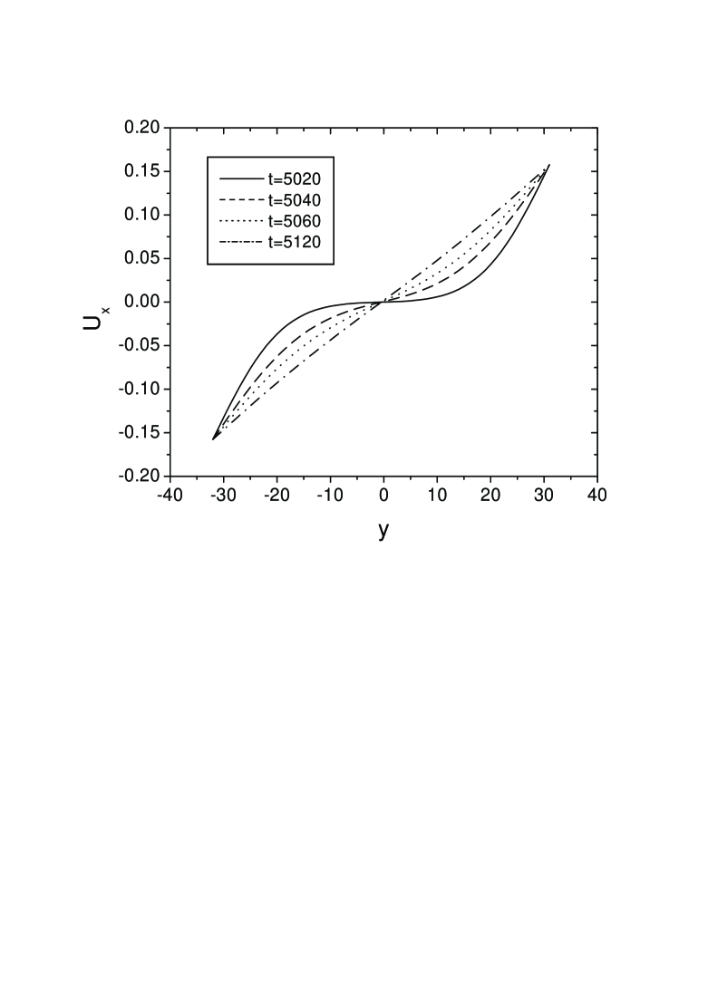
FIG. 1.: Relaxation process of the horizontal velocity profile for the symmetric binary fluids, where $\tau=2$, $L=64$, $t_{on}=5000$. The corresponding times are shown in the inset.

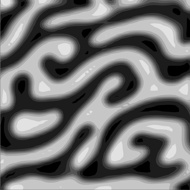
FIG. 2.: The configuration of the field $\varphi$ at the time $t=5120$, the parameters are the same as in Fig.1. From dark to white, the value of $\varphi$ varies in the scope $-1.0\leq\varphi\leq 1.0$.

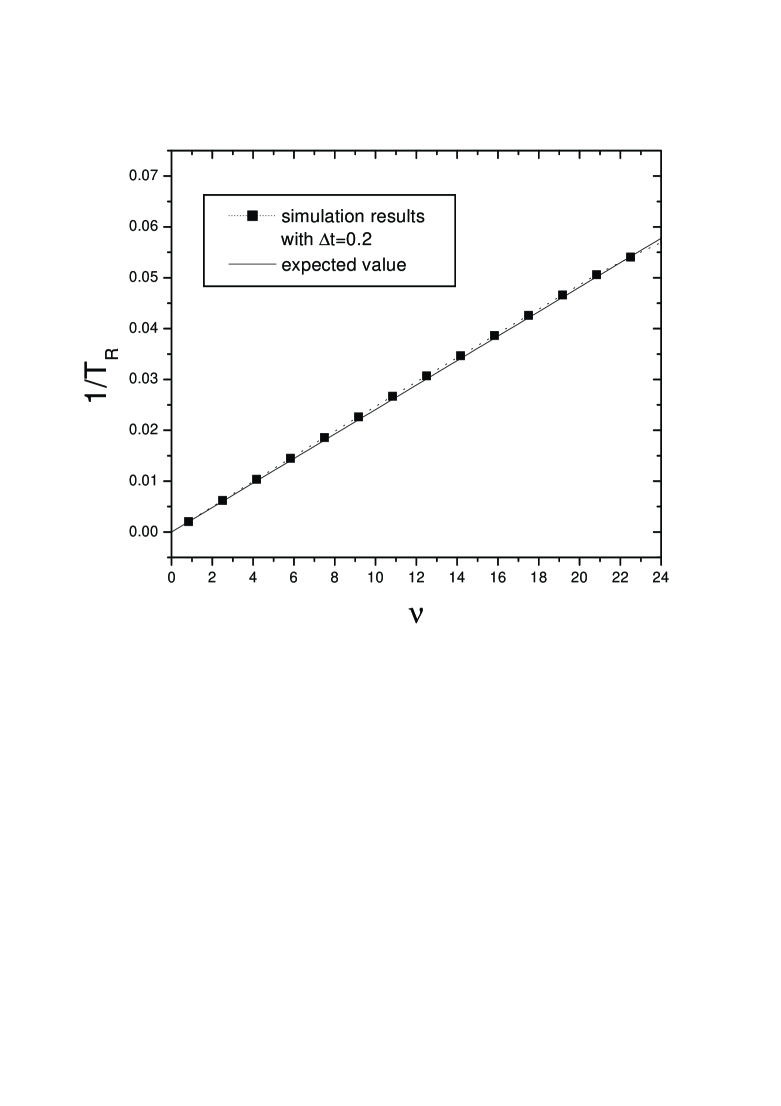
FIG. 3.: $1/T_{R}$ as a function of $\nu$. The lattice size $L=128$ is used in the simulation. The dotted line with symbols correspond to the simulation results and the solid line shows the expected values from the definition (15).

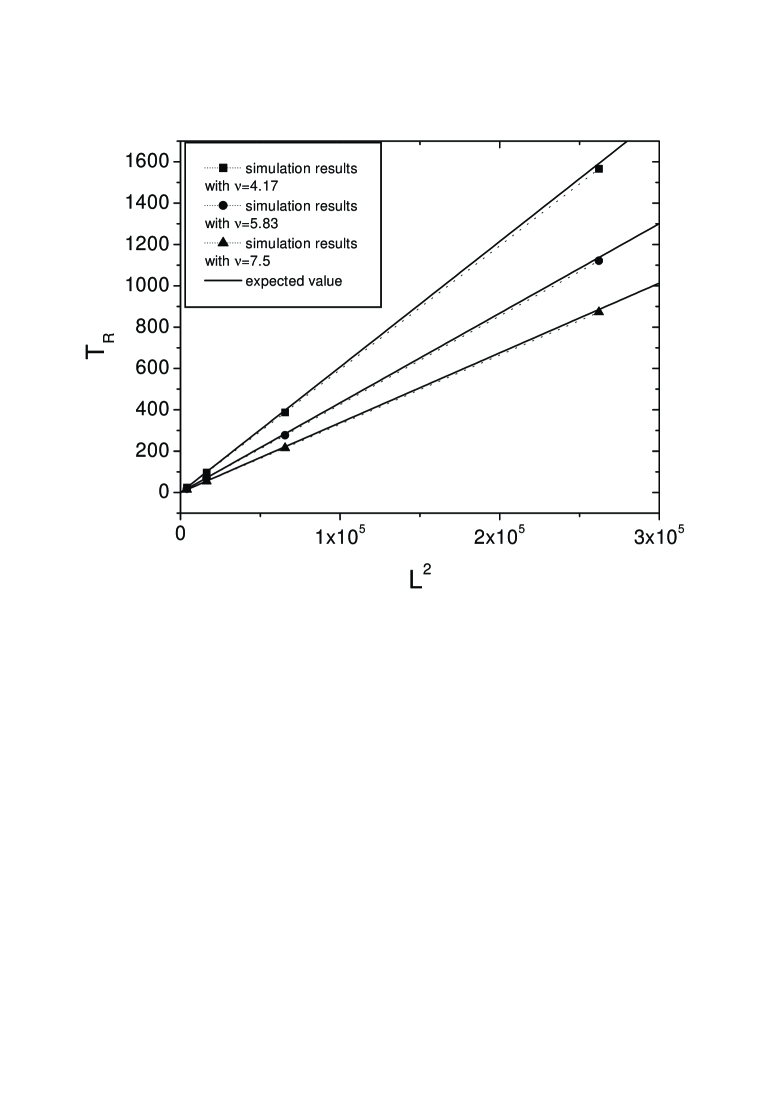
FIG. 4.: $T_{R}$ as a function of $L^{2}$. The dotted lines with symbols show the simulation results and the solid lines show the expected values from the definition (15). The four points in each case correspond to cases of $L=64$, $128$, $256$, and $512$. The simulation step in this figure is $\Delta t=0.2$.

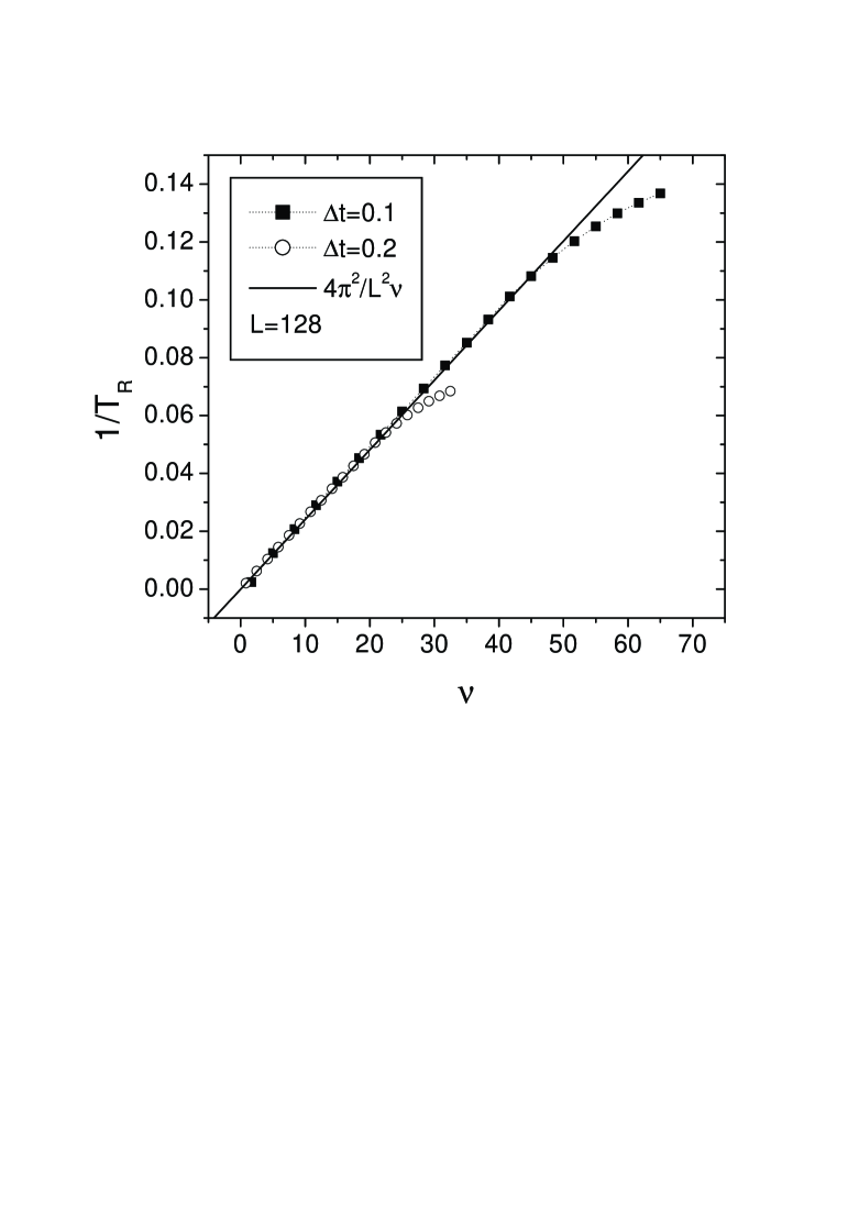
FIG. 5.: Two simulation results for $1/T_{R}$ as a function of $\nu$, where the expected value of $1/T_{R}$ is also shown to guide the eyes. The lattice size and time steps used in the simulations are shown in the inset.

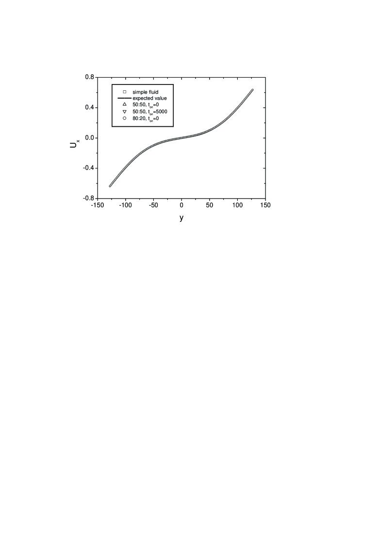
FIG. 6.: Simulation and expected results of the velocity profiles, where $L=256$, $\tau=2$ ($\nu=2.5$), $t-t_{on}=600$. The solid line shows the expected values from Eq. (14) with $n=1$. The symbols show the simulation results. The type of the fluid and the value of $t_{on}$ are shown in the inset.

REFERENCES

- [1] See, e.g., R. G. Larson, The Structure and Rheology of Complex Fluids (Oxford University Press, New York, 1999).
- [2] A. Onuki, J. Phys. Cond. Matter 9, 6119 (1997).
- [3] Aiguo Xu, G.Gonnella and A.Lamura, conden-mat/0211085; to appear in Phys. Rev. E.
- [4] A.J.Bray, Adv. Phys. 43, 357 (1994).
- [5] J.S.Rowlinson and B.Widom, Molecular Theory of Capillarity (Clarendon Press, Oxford, 1982).
- [6] A.J.M.Yang, P.D.Fleming, and J.H.Gibbs, J. Chem. Phys. 64, 3732 (1976).
- [7] R.Evans, Adv. Phys. 28, 143 (1979).
- [8] E.Orlandini, M.R.Swift, and J.M.Yeomans, Europhys. Lett. 32, 463 (1995).
- [9] M.R.Swift, E.Orlandini, W.R.Osborn, and J.M.Yeomans, Phys. Rev. E 54, 5041 (1996).
- [10] P. Bhatnagar, E.P. Gross, and M.K.Krook, Phys. Rev. 94, 511 (1954).
- [11] H.Chen, S.Chen, and W.Matthaeus, Phys. Rev. A 45, R5339 (1992).
- [12] E.Orlandini, M.R.Swift, and J.M.Yeomans, Europhys. Lett. 32, 463 (1995).
- [13] M.R.Swift, E.Orlandini, W.R.Osborn, and J.M.Yeomans, Phys. Rev. E 54, 5041 (1996).
- [14] S.Chapman and T.Cowling, The Mathematical Theory of Non-uniform Gases (Cambridge University Press, Cambridge, 1970).
- [15] P.Lavalée, J.Boon and A.Noullez, Physica D 47, 233 (1991).
- [16] R. Cornubert, D. d’Humieres, and D. Levermore, Physica D, 47, 241 (1991).
- [17] A.Lamura and G.Gonnella, Physica A 294, 295 (2001).
- [18] H.Schlichting, Boundary Layer Theory (McGraw-Hill series in Mechanical Engineering, 1979).
- [19] J.C.Desplat, I.Pagonabarraga, and P.Bladon, Comp. Phys. Comm. 134, 273 (2001).
- [20] A.J.Briant, Papatzacos, and J.M.Yeomans, Phil. Trans. R. Soc. London 360, 485 (2002).