Compensation for Extreme Outages caused by Polarization Mode Dispersion and Amplifier noise

Vladimir Chernyak^a, Michael Chertkov^b, Igor Kolokolov^b,c,d, and Vladimir Lebedev^b,c

^aCorning Inc., SP-DV-02-8, Corning, NY 14831, USA;

^bTheoretical Division, LANL, Los Alamos, NM 87545, USA;

^cLandau Institute for Theoretical Physics, Moscow, Kosygina 2, 117334, Russia;

^dBudker Institute of Nuclear Physics, Novosibirsk 630090, Russia.

Abstract

Joint effect of weak birefringent disorder and amplifier noise on transmission in optical fiber communication systems appears to be strong. The probability of an extreme outage that corresponds to anomalously large values of Bit Error Rate (BER) is perceptible. We analyze the dependence of the Probability Distribution Function (PDF) of BER on the first-order and also higher-order PMD compensation schemes.

© 2024 Optical Society of America
OCIS codes: (060.0060) Fiber Optics and Optical Communication
(030.6600) Statistical Optics

Introduction: Polarization Mode Dispersion (PMD) is recognized to be a substantial impairment for optical fiber systems with the $40$-Gbs/s and higher transmission rates. One may not have a complete control of PMD since the fiber system birefringence is changing substantially under the influence of environmental condition (e.g., stresses and temperature) fluctuations, see e.g. [1, 2]. Thus, dynamical PMD compensation became a major issue in modern fiber optics communication technology [3, 4]. Development of experimental techniques capable of the first- [5, 6, 7] and higher-orders [7, 8] PMD compensation have raised a question of how to evaluate the compensation success (or failure). Traditionally, the statistics of the PMD vectors of first [9, 10, 11] and higher orders [12, 13, 14] is considered as a measure for any particular compensation method performance. However, these objects are only indirectly related to what actually represents the fiber system reliability. In this letter we show that the PMD effects should be considered jointly with impairments due to amplifier noise, since fluctuations of BER caused by variations of the birefringent disorder, are substantial. We demonstrate that probability of extreme outages is much larger than one could expect from naive estimates singling out effects of either of the two impairments. This phenomenon is a consequence of a complex interplay between the impairments of different natures. (Birefringent disorder is frozen, i.e. it does not vary on all propagation related time scales, while the amplifier noise is extremely short-correlated.) The effect may not be explained in terms of just an average value of BER, or statistics of any PMD vectors of different orders, but rather should be naturally described in terms of the PDF of BER, and specifically its tail. A consistent theoretical approach to calculating the tail will be explained briefly, with a prime focus on the analysis of the first- and higher-order compensation effects on the extreme outages measured in terms of the PDF of BER.

Bit-Error-Rate: We consider the so-called return-to-zero modulation format, when pulses (information carriers) are well separated in time, $t$. The quantity measured at the output of the optical fiber line is then pulse intensity:

$$I=\int\mathrm{d}t\,G(t)\left|{\cal K}\bm{\varPsi}(Z,t)\right|^{2}\,,$$ (1)

where $G(t)$ is the convolution of the electrical (current) filter function with the sampling window function. The two-component complex field $\bm{\varPsi}(Z,t)$ describes the output signal envelope. The two components correspond to two polarizations of the optical fiber mode. The linear operator ${\cal K}$ in Eq. (1) stands for a variety of engineering “tricks” applied to the output signal. They consist of the optical filter ${\cal K}_{f}$, and the compensation ${\cal K}_{c}$ parts, respectively, assuming the compensation is applied first followed by filtering, i.e. ${\cal K}={\cal K}_{f}\times{\cal K}_{c}$. Ideally, $I$ accepts two different values depending on whether the information slot is vacant or filled. However, the impairments enforce deviations of $I$ from the fixed values. Therefore, one has to introduce a threshold (decision level) $I_{d}$ and declare that the signal encodes “1” if $I>I_{d}$ and is related to “0” otherwise. Sometimes the information is lost, i.e. an initial “1” is detected as a “0” at the output or vise versa. BER is the probability of such “error” event (with statistics being collected over many pulses coming through a fiber with a given realization of birefringent disorder). For successful system performance the BER must be extremely small, i.e. both impairments typically cause only small distortions to a pulse. It is straightforward to verify that anomalously high values of BER originate solely from the “$1\to 0$” events. We denote the probability of such events by $B$. Non-zero $B$ are caused by the noise, the values, however, depending on particular realization of the birefringent disorder.

Noise averaging: We consider the linear propagation regime, when the output signal $\bm{\varPsi}$ can be decomposed into two contributions: $\bm{\varphi}$, related to a noiseless initial pulse evolution and the noise-induced $\bm{\phi}$ part of the signal. $\bm{\phi}$ appears to be a zero-mean Gaussian variable (insensitive to a particular birefringence and chromatic dispersion in the fiber) and is completely characterized by the pair correlation function

$$\langle\phi_{\alpha}(Z,t_{1})\phi^{\ast}_{\beta}(Z,t_{2})\rangle=D_{\xi}Z\delta_{\alpha\beta}\delta(t_{1}-t_{2}).$$ (2)

Here, $Z$ is the total length of the fiber line, and the product $D_{\xi}Z$ is the amplified spontaneous emission (ASE) spectral density accumulated along the line. The coefficient $D_{\xi}$ is introduced into Eq. (2) to reveal the linear growth of the ASE factor with $Z$ [15].

Disorder averaging: The noise-independent part of the signal is

$$\bm{\varphi}=e^{i\eta\partial_{t}^{2}}\hat{U}\bm{\varPsi}_{0}(t)\,,\quad\hat{U}=T\!\exp\left[\int_{0}^{Z}\!\!\!\mathrm{d}z\,\hat{m}(z)\partial_{t}\right],$$ (3)

where $\bm{\varPsi}_{0}(t)$, $\eta=\int_{0}^{Z}\!\!\!\mathrm{d}z\,d(z)$, $z$, and $d(z)$ are the input signal profile, the integral chromatic dispersion, coordinate along the fiber, and the local chromatic dispersion, respectively. The ordered exponent $\hat{U}$ depends on the $2\times 2$ matrix $\hat{m}(z)$ that characterizes the birefringent disorder. The matrix can be represented as $\hat{m}=h_{j}\hat{\sigma}_{j}$, $h_{j}(z)$ being a real three-component field and $\hat{\sigma}_{j}$ the Pauli matrices. Averaging over many states of the birefringent disorder any given fiber is going through (birefringence varies on a time scale much longer than any time scale related to the pulse propagation through the fiber), or over instant states of birefringence in different fibers, one finds that $h_{j}(z)$ is a zero-mean Gaussian field described by the following pair correlation function

$$\langle h_{i}(z_{1})h_{j}(z_{2})\rangle=D_{m}\delta_{ij}\delta(z_{1}-z_{2}).$$ (4)

If birefringent disorder is weak the integral $\bm{H}=\int_{0}^{Z}\mathrm{d}z\,\bm{h}(z)$ coincides with the PMD vector. Thus, $D_{m}=k^{2}/12$, where $k$ is the so-called PMD coefficient.

PDF of BER is the proper object to describe fluctuations of $B$ caused by the birefringent disorder. For successful fiber system performance the BER should be extremely small, i.e. typically both impairments can cause only small distortions of a pulse. Stated differently, the optical signal-to-noise ratio (OSNR) and the ratio of the squared pulse width to the mean square value of the PMD vector are both large. OSRN can be estimated as $I_{0}/(D_{\xi}Z)$ where $I_{0}=\int\mathrm{d}t\,|\varPsi_{0}(t)|^{2}$ is the initial pulse intensity, and the integration goes over a single slot populated by an ideal (initial) pulse, encoding “1”. Since the value of OSNR is large averaging over the noise can be performed using the saddle-point method. This leads to a conclusion that $D_{\xi}Z\ln B$ depends on the birefringence, shape of the initial signal and the details of the compensation and measurement procedures, being, however, independent of the noise. Typically, $B$ fluctuates around $B_{0}$, the zero-disorder, $h_{j}=0$, value of $B$. For any finite value of $\bm{h}$ one gets, $\ln(B/B_{0})=\Gamma I_{0}/(D_{\xi}Z)$, where the dimensionless factor $\Gamma$ depends on $\bm{h}$. Since the noise is weak, even small disorder can generate strong increase in $B$. This implies that a perturbative calculation of $\Gamma$ based on expanding the ordered exponent $\hat{U}$ in Eq. (3) in powers of $\hat{m}$, describes the most essential part of the PDF of $B$. Thus, in the situation when no compensation is applied one derives $\Gamma=\mu_{1}H_{3}/b$, whereas in the simplest case of the “setting the clock” compensation, accounting for the average (typical) temporal shift, one arrives at $\Gamma=\mu_{2}(H_{1}^{2}+H_{2}^{2})/b^{2}$, $b$ being the pulse width and $\mu_{1,2}$ being dimensionless coefficients.

Long tail: The PDF of $B$, ${\cal S}(B)$ (that appears in the result of averaging over many realizations of the birefringent disorder) can be found by recalculating the statistics of $H_{j}$ using Eq. (4) followed by substituting the result into the corresponding expression that relates $B$ to $H_{j}$. Our prime interest is to describe the PDF tail that corresponds to the values of $H_{j}$ substantially exceeding their typical value $\sqrt{D_{m}Z}$ remaining, however, much smaller than the signal duration $b$. In this range one gets the following estimates for the differential probability ${\cal S}(B)\,\mathrm{d}B$:

$$a)\ \exp\left[-\frac{D_{\xi}^{2}Zb^{2}}{2D_{m}\mu_{1}^{2}I_{0}^{2}}\ln^{2}\left(\frac{B}{B_{0}}\right)\right]\frac{dB}{B},\quad b)\ \frac{B_{0}^{\alpha}\,\mathrm{d}B}{B^{1+\alpha}}\,,$$ (5)

where (a) corresponds to the no-compensation situation, (b) stands for the optimal “setting the clock” case, and $\alpha\equiv D_{\xi}b^{2}/(2\mu_{2}D_{m}I_{0})$. Note, that the result in the case (b) shows a steeper decay compared to the case (a), which is a natural consequence of the “setting the clock” compensation.

PMD compensation: One deduces from Eqs. (1,3) that the output intensity depends on the birefringent disorder via the factor ${\cal K}_{c}\hat{U}$. The idea of the compensation can be restated in a more formal way as building a linear operator ${\cal K}_{c}$ that suppresses the dependence of ${\cal K}_{c}\hat{U}$ on $\bm{h}$. The so-called first-order compensation ${\cal K}_{c}={\cal K}_{1}$

$${\cal K}_{1}=\exp\left(-\int_{0}^{Z}\!\!\!\mathrm{d}z\,h_{j}\hat{\sigma}_{j}\partial_{t}\right)\,,$$ (6)

boils down to compensating the first term in the expansion of the ordered exponential $\hat{U}$ in $\bm{h}$ [12, 13, 14]. Technically, this is achieved by sending the signal aligned with either of the two principal polarization states of the fiber [5], or inserting a PMD controller (a piece of polarization maintaining fiber with uniformly distributed well-controlled birefringence) at the receiver [6]. Expanding ${\cal K}_{1}\hat{U}$ in $\bm{h}$ followed by substituting the result into Eq. (1) and evaluating $B$ leads to

$$\Gamma=(\mu^{\prime}_{2}/b)^{2}\int_{0}^{Z}\!\!\!\mathrm{d}z^{\prime}\int_{0}^{z^{\prime}}\!\!\!\mathrm{d}z\left[h_{1}(z^{\prime})h_{2}(z)\!-\!h_{2}(z^{\prime})h_{1}(z)\right],$$ (7)

$b$ being the pulse width, and only the leading $O(h^{2})$ term is retained in Eq. (7). The dimensionless coefficient $\mu^{\prime}_{2}$ is related to the output signal chirp, produced by the initial signal chirp and/or the nonzero integral chromatic dispersion $\eta$. Recalculating the statistics of $\Gamma$ using Eqs. (4,7) one obtains the following tail ${\cal S}(B)$ for the PDF of $B$

$${\cal S}(B)\,\mathrm{d}B\sim\frac{B_{0}^{\gamma}\,\mathrm{d}B}{B^{1+\gamma}},\qquad\gamma\equiv\frac{\pi D_{\xi}b^{2}}{2|\mu^{\prime}_{2}|D_{m}I_{0}},$$ (8)

and Eq. (8) holds when $\ln(B/B_{0})\gg|\mu^{\prime}_{2}|D_{m}I_{0}/[D_{\xi}b^{2}]$.

Non-chirped signal: If the output signal is not chirped $\mu^{\prime}_{2}=0$ and the first non-vanishing term in the expansion of $\Gamma$ in $h_{j}$ is of the third order. Expanding ${\cal K}_{1}\hat{U}$ up to the leading (third order) term yields

$$\Gamma=\frac{\mu_{3}}{b^{3}}\!\int_{0}^{Z}\!\!\!\!\mathrm{d}z_{1}\!\int_{0}^{z_{1}}\!\!\!\!\mathrm{d}z_{2}\!\int_{0}^{z_{2}}\!\!\!\mathrm{d}z_{3}\,\Bigl{\{}2h_{3}(z_{1}){\cal H}(z_{2},z_{3})\!-\!h_{3}(z_{2}){\cal H}(z_{1},z_{3})\!-\!h_{3}(z_{3}){\cal H}(z_{1},z_{2})\Bigl{\}},$$ (9)

with ${\cal H}(z_{1},z_{2})=h_{1}(z_{1})h_{1}(z_{2})+h_{2}(z_{1})h_{2}(z_{2})$. Substituting Eq. (9) into the expression for $B$ in terms of $\Gamma$ and making use of Eq. (4) leads to a representation of the PDF of $B$ as a path-integral over $\bm{h}$. Integrating over $h_{3}$ explicitly and approximating the resulting integral over $h_{1,2}$ by its saddle-point value, one finds the PDF tail

$$\ln{\cal S}\approx-4.2\frac{(D_{\xi}Z/I_{0})^{2/3}b^{2}}{\mu_{3}^{2/3}D_{m}Z}\left(\ln\frac{B}{B_{0}}\right)^{2/3}.$$ (10)

Eq. (10) is valid at $D_{\xi}Z\ln(B/B_{0})\gg\mu_{3}(D_{m}Z)^{3/2}I_{0}/b^{3}$.

Simple model: The dimensionless coefficients $\mu^{\prime}_{2}$, $\mu_{3}$ can be computed in the framework of a simple model, with the decision level threshold $I_{d}$ being twice smaller than the ideal intensity, the Lorentzian profile of optical filter, ${\cal K}_{f}\bm{\varPsi}=\int_{0}^{t}\mathrm{d}t^{\prime}\exp[-t/\tau]\bm{\Psi}(t-t^{\prime})/\tau$, and the step function form for $G$, $G(t)=\theta(T-|t|)$. We also consider a Gaussian weakly-chirped initial signal $\bm{\varPsi}_{0}\propto\exp(-t^{2}/[2b^{2}])(1+i\beta_{in}t^{2}/b^{2})$, $\beta_{in}\ll 1$ (here both the signal amplitude and its width are re-scaled to unity). The output signal chirp becomes $\beta=\beta_{in}+\eta$, $\eta$ being the integral dimensionless chromatic dispersion. Then, $\mu^{\prime}_{2}$ is proportional to $\beta$, and the slope $\mu^{\prime}_{2}/\beta$, found from the saddle-point equations numerically, along with corresponding values of $\Gamma_{0}\equiv-D_{\xi}z\ln B_{0}/I_{0}$ and $\mu_{1,2,3}$ are shown in Fig. 1 for a reasonable range of the parameters $T,\tau$ (measured in the units of the pulse width $b$).

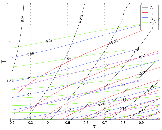
Fig. 1: Dependence of $\Gamma_{0}=-D_{\xi}z\ln B_{0}/I_{0}$, $\mu_{1}$, $\mu_{2}$, $\mu^{\prime}_{2}/\beta$ and $\mu_{3}$ on $T,\tau$, for the model explained in the text. All quantities are measured in the units corresponding to the pulse width and amplitude both equal to one.

Advanced compensation: The fiber system performance can be improved even further. First of all, special filtering efforts can enforce the output pulse symmetry under the $t\to-t$ transformation. Then the $O(H^{3})$ contribution to $\Gamma$ will also be cancelled out and Eq. (9) will be replaced by $\Gamma=O(H^{4})$. Second, one can use a more sophisticated compensation ${\cal K}_{c}$ aiming to cancel as much terms in the expansion of ${\cal K}_{c}\hat{U}$ in $\bm{h}$ as possible. This approach corresponds to the so-called high-order compensation techniques implemented experimentally in many modern setting (see e.g., [7, 8]). The high-order compensation can substantially reduce the dependence of $\Gamma$ on $\bm{h}$, leading to $\Gamma\sim\mu_{k}(H/b)^{k}$ (where $k$ exceeds by one the compensation degree if no additional cancellations occur). In this case the tail of the PDF of $\Gamma$ is estimated by $\exp[-(b^{2}/D_{m}Z)(\Gamma/\mu_{k})^{2/k}]$. This results in the following expression for the tail of the PDF of $B$,

$$\ln{\cal S}\sim-(b^{2}/D_{m}Z)[\mu_{k}^{-1}D_{\xi}Z\ln(B/B_{0})/I_{0}]^{2/k},$$ (11)

valid for $D_{\xi}Z\ln(B/B_{0})\gg(D_{m}Z/\mu_{k}b^{2})^{k/2}I_{0}$. Eq. (11) generalizes Eqs. (8,10). One concludes that, as anticipated, the compensation does suppress the PDF tail. One also finds the outage probability ${\cal O}$, defined as ${\cal O}=\int^{1}_{B_{\ast}}\mathrm{d}B\,{\cal S}(B)$ (with $B_{\ast}$ being some fixed value much larger than $B_{0}$), $\ln{\cal O}\sim-[(\mu_{k}I_{0})^{-1}D_{\xi}Z\ln(B_{\ast}/B_{0})]^{2/k}b^{2}/(D_{m}Z)$.

Example: Summarizing, our major result is quantitative description of the suppression of the extremely long tail in the PDF of BER. We find it useful to conclude with presenting a numerical example that corresponds to a case relevant for the optical fiber communications. Consider a fiber line with $\Gamma_{0}=0.06$, $\mu_{1}=0.06$, $\mu_{2}=0.12$, $\mu^{\prime}_{2}=0.15$ and $\mu_{3}=0.35$, which is also characterized by typical bit-error probability, $B_{0}=10^{-12}$ that corresponds to $I_{0}/[D_{\xi}Z]\approx 460$. We also assume that the PMD coefficient, $k=\sqrt{12D_{m}}$, is $0.2$ $ps/\sqrt{km}$, the pulse width is $b=25$ $ps$, and the system length is $Z=2,500$ $km$, i.e. $D_{m}Z/b^{2}\approx 0.013$. Then the outage probability corresponding to $B_{\ast}=10^{-10}$, that is the probability for $B$ to be at least $2$ orders of magnitude larger than $B_{0}$, is ${\cal O}\approx 0.35$ if no compensation is applied, see Eq. (5a), while one derives ${\cal O}\approx 0.04$, ${\cal O}\approx 4\cdot 10^{-4}$ and ${\cal O}\approx 2\cdot 10^{-13}$ for Eq. (5b), Eq. (8) and Eq. (10), describing the cases of the “setting the clock”, first- and second-order compensations, respectively.

Acknowledgment: We are thankful to I. Gabitov for numerous valuable discussions. We also wish to acknowledge the support of LDRD ER on “Statistical Physics of Fiber Optics Communications” at LANL.