Prospects for Forbidden-Transition Spectroscopy and Parity Violation Measurements
using a Beam of Cold Stable or Radioactive Atoms

Abstract

Laser cooling and trapping offers the possibility of confining a sample of radioactive atoms in free space. Here, we address the question of how best to take advantage of cold atom properties to perform the observation of as highly forbidden a line as the 6S-7S Cs transition for achieving, in the longer term, Atomic Parity Violation measurements in radioactive alkali isotopes. Another point at issue is whether one might do better with stable, cold atoms than with thermal atoms. To compensate for the large drawback of the small number of atoms available in a trap, one must take advantage of their low velocity. To lengthen the time of interaction with the excitation laser, we suggest choosing a geometry where the laser beam exciting the transition is colinear to a slow, cold atomic beam, either extracted from a trap or prepared by Zeeman slowing. We also suggest a new observable physical quantity manifesting APV, which presents several advantages: specificity, efficiency of detection, possibility of direct calibration by a parity conserving quantity of a similar nature. It is well adapted to a configuration where the cold atomic beam passes through two regions of transverse, crossed electric fields, leading both to differential measurements and to strong reduction of the contributions from the $M_{1}$-Stark interference signals, potential sources of systematics in APV measurements. Our evaluation of signal to noise ratios shows that with available techniques, measurements of transition amplitudes, important as required tests of Atomic Theory should be possible in ¹³³Cs with a statistical precision of $10^{-3}$ and probably also in Fr isotopes for production rates of $\gtrsim 10^{6}$ Fr atoms s^-1. For APV measurements to become realistic, some practical realization of the collimation of the atomic beam as well as multiple passages of the excitation beam matching the atomic beam looks essential.

I Introduction : Motivations

Atomic Parity Violation (APV) measurements have proved successful for probing at low energy one of the most fundamental predictions of the Standard Model (SM), namely the existence of a weak electron-nucleus interaction mediated by the exchange of neutral gauge bosons $Z_{0}$ [1, 2, 3]. Up to now the efforts have been focused on the comparison between the experimental determination of the weak charge of the atomic nucleus, $Q_{W}$, and its SM prediction at the 0.5$\%$ level of precision, the cesium atom lending itself to the most precise comparison [4, 5, 6]. Actually, it looks somewhat too early to assert definitely either the absence or existence of a deviation, most likely less than 2.5 $\sigma$ [6, 7]. On the other hand, it has not been possible, yet, to test another important SM prediction concerning the variation of $Q_{W}$ along a string of isotopes belonging to the same element. An original experimental approach is currently pursued for rare-earth elements namely Yb [8] and Dy[9], but it also would be extremely valuable to extend the measurements which have proved successful for natural cesium, ¹³³Cs (the sole stable Cs isotope), to a few of its numerous radioactive isotopes, as well as to other alkali isotopes, more excitingly radioactive francium. With Z=87, francium is expected to lead, due to the fast increase with Z [1], to APV effects 18 times larger than cesium, while it does not look unrealistic to have a theoretical prediction of its weak charge as precise as that for cesium [10]. Indeed, atomic structure calculations for alkali are (barring H and He) the most precise available. This, added to the fact that many isotopes can be produced, makes this element often considered as one of the most interesting candidates for forthcoming experiments. Moreover, since up to now, the nuclear anapole moment [11] has been detected only for ¹³³Cs [2] (an even neutron-number isotope), it is important to measure it for another isotope (preferably one with an odd neutron-number). Regardless of APV, measurements on the forbidden line in alkali-metal atoms are important since forbidden magnetic dipole amplitudes are “the most sensitive among electromagnetic transition amplitudes to the accuracy of the relativistic description of an atomic system” [12], i.e. rigorous tests of atomic theory.

Francium, and more generally short-lived radioactive atoms, either obtained from a radioactive source or produced on line by an accelerated ion beam colliding a target, are produced at a limited rate, with a thermal, or even superthermal, velocity distribution. In order to perform APV measurements the first prerequisite is to avoid their spreading out in space and their loss inside the wall. Only the radiative cooling and trapping techniques [13] possibly combined with Light Induced Atomic Desorption (LIAD) [14] can succeed in this kind of operation. Several successful attempts to load radioactive alkali atoms in a neutral atom trap have been reported with ²¹Na [15], ³⁸K^m, ³⁷K [16], ⁷⁹Rb [17], ¹³⁵Cs [18], ^207-211Fr [19], ²²¹Fr [20]. Observation of several allowed Fr transitions has been realized for atoms trapped inside a MOT, leading to precise spectroscopic measurements [21]. But never, yet, has it been reported for a transition as highly forbidden as the Fr 7S-8S transition. Therefore, before attempting APV measurements with cold atoms, a preliminary - and by no means straightforward - objective consists in observing the 6S-7S transition with trapped Cs atoms. Since the precise value of the parity conserving transition amplitudes, in particular the Stark induced amplitude associated with the vector polarizability $\beta$, is still a somewhat open question (see below), as an assessment of the potential of trapped atoms for this kind of experiment, we suggest a new precision measurement of the ratio $M_{1}^{hf}/\beta$. Here, the magnetic dipole amplitude $M_{1}^{hf}$ induced by hyperfine interaction serves as a precisely known amplitude used for calibration [22, 23]. This would be all the more precious since the previous measurements [3] were made in acrobatic conditions (background equal to 100 times the signal [3]) and have led to a result for $\beta$ which differs from a recent independent semi-empirical determination by (0.7 $\pm$ 0.4)$\%$ [24]. Though small, such a difference is sufficient to narrow the gap between theoretical and experimental values of $Q_{W}({\rm Cs})$ from 2.2 to 0.9$\sigma$. A measurement of $M_{1}^{hf}/\beta$ in cesium will allow us to assess the feasibility of similar measurements in francium, knowing the production rate. Finally, we also attempt to evaluate the feasibility of an even more ambitious project, namely a new high precision measurement of the parity violating electric dipole amplitude $E_{1}^{pv}$ in cesium, and hence $Q_{W}({\rm Cs})$ by an independent method using cold atoms. Indeed, such an independent measurement would be extremely valuable as a cross check of this fundamental quantity [25]. Beyond this, we cannot understate how welcome a measurement of $Q_{W}({\rm Fr})$ would be, if some day feasible.

Our paper is a prospective work suggesting preparatory experiments for much more ambitious projects. Once a sample of cold alkali atoms is produced at the center of a trap, there remains a still unsolved point at issue : what is the best way to use it for exciting and probing the forbidden Cs 6S-7S transition, or the analogous 7S-8S transition in Fr, in the Stark electric field necessary to previous APV measurements? Even for the stable isotope ¹³³Cs, the biggest difficulty is linked to the small number of atoms available in a trap. It is the purpose of the present paper to quantify such a difficulty by making comparisons with conditions realized in previous APV experiments performed with stable, thermal atoms and to suggest an experimental approach using their different specific properties. We suggest advantageous means to exploit their low velocity and we also propose a new physical observable which, we believe, is well adapted to this situation. It is shown to be well suited to the measurement of first $M_{1}^{hf}/\beta$ and later $E_{1}^{pv}/M_{1}^{hf}$. Concerning the measurement accuracy, in an approach of this kind two parameters play an essential role : i) the number of atoms present at a given time in the interaction region, ii) the probability for such an atom to contribute to the APV signal, which takes into account the nature of the physical observable, and both the excitation and detection efficiencies. We have not found the ideal compromise between simplicity and outstanding performances, transferable from Cs to Fr. According to the exact goal to be reached the experimental scheme to be chosen will probably have to change. We consider three different experimental approaches, all of them relying on the production of a cold, slow atomic beam. They differ by the method of production of the beam and its parameters. This will appear explicitly in §II. The observable physical quantity is presented in §III, while §IV describes a method to suppress the dangerous systematic effect which might arise from the Stark-$M_{1}$ interference effect when one wants to measure $E_{1}^{pv}$. Finally (§V), we make predictions for the Signal to Noise ratio for measuring the interesting physical quantities mentioned above, in these three different, well-defined and realistic, experimental configurations.

II Use of a slow and cold atomic beam excited by a colinear laser beam

The energy levels and wavelengths relevant to APV measurements and to laser trapping operation for both cesium and francium are shown on Fig. 1. A precise value of the measured energy difference between the Fr 8S_1/2 and 7S_1/2 levels is given in [26]. Performing the PV measurements inside an optical molasses or a Magneto Optical Trap (MOT), precisely where the atoms are cooled and stored presents some inconvenience. Indeed, both laser cooling and APV measurements require specific conditions which look difficult to reconcile : for instance, the presence of excited atomic species in the interaction region and the interception of the wide cooling light beams by the necessary electrodes are both difficult to avoid. Among a large variety of techniques available for manipulating atomic velocities by electromagnetic forces [27], several of them offer the possibility of producing a well collimated beam of slow, cold atoms. In order to concentrate the discussion on a well defined situation, we shall choose the example of a pyramidal MOT built according to the judicious and simple suggestion of Lee et al. [28], now used by several groups [29, 30]. The trap is built with four mirrors, standing as the four faces of an inverted pyramid. A single cooling beam, circularly polarized, is enough to create, after reflexion on the four mirrors, the same field configuration as a standard six-beam MOT. When the pyramidal trap is vapor-loaded, a beam of slow and cold atoms escapes continuously through the hole bored through the pyramid apex because of local imbalance of intensities. In typical conditions this kind of device can provide a continuous flux $\Phi_{at}$ of $\gtrsim 2\times 10^{9}$ cesium atoms/s with a mean velocity $v$ tunable around 10 m/s and a velocity spread less than 1.5 m/s [30]. The transverse velocity spread of the beam is found to lie close to the Doppler transverse limit for cesium $\sqrt{\hbar\Gamma/m}=0.13$ m/s.

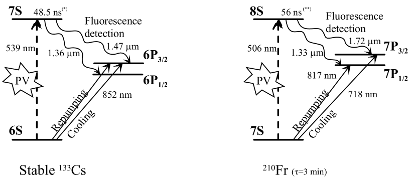
FIG. 1.: Energy levels and wavelengths relevant for APV experiments and atomic cooling and trapping in cesium and francium. $(^{\star})$ Cs 7S state lifetime from experiment [31], and $(^{\star\star})$ Fr 8S state lifetime from theory [32].

The pyramidal trap has advantages of low cost and simplicity, but still better performances can be achieved with more sophisticated devices. In particular, ref.[33, 34] describes how an even slower and colder rubidium beam can be obtained using a vapor loaded laser trap which ensures two-dimensional magneto-optical trapping, as well as longitudinal cooling by a moving molasses (MM-MOT). The average velocity can be as low as 1m/s and the velocity distribution has been evaluated: $\Delta v/v<1/10$. When either one of those slow atomic beams is illuminated by a co- or counter-propagating narrow line-width cw laser beam, the dispersion of the longitudinal velocities is small enough for all atoms excited on the 6S-7S transition to belong to a single velocity class. Moreover, at optimum alignment, the divergence of the atomic beam (26 mrd FWHM) going out of the pyramidal trap is small enough for avoiding any significant atom loss out of a 1 mm radius laser beam over an interaction length of 4 cm. In contrast, the larger divergence of the ultra cold beam [34] unavoidably complicates the design of the experiment (see proposal 2, §V B). Other 2D-MOT, among those delivering larger atomic fluxes [35, 36, 37], have, for the present application, the drawback of either a larger divergence or a larger velocity spread. On the other hand, the features needed here, high flux, moderate velocity and low divergence are met by other techniques, namely Zeeman slowing. In particular, the Zeeman-slower apparatus described in ref [38] has very attractive features : flux of Cs atoms exceeding 10¹⁰ s^-1, very small spread of longitudinal velocities, $\sim$ 1 m/s and much better collimation (divergence angle less than 1 mrd). This gives the possibility of lengthening the interaction region (see proposal 3 in Table I and §V C). Although some adaptation will be necessary to make the system work with radioactive isotopes, depending on their method of production, it is interesting to evaluate its potentiality as compared to that of a thermal atomic beam or a vapor cell.

After a short path beyond the trap exit (or the collimation module [38]), the atomic beam enters the interaction region which includes capacitor plates generating the Stark field, with the plane electrodes parallel to the beam direction. The first relevant parameter to be compared here to previous experimental configurations is the number of atoms $N_{at}$ interacting with the excitation laser beam in the interaction region of length $l$.

For an atomic beam experiment $N_{at}=\Phi_{at}\times l/v$. For a vapor at thermal equilibrium (Paris experiment [40]) we take into account that only a fraction of the atoms can absorb the resonant light beam which has a spectral width much smaller than the Doppler width. By averaging the velocity-dependent transition probability over the thermal distribution, one finds that this can be accounted for by the reduction factor : $R=\sqrt{2\pi}\Gamma/4\Gamma_{D}$ (see ref. [41]), where $\Gamma_{D}=\omega_{0}\sqrt{\frac{kT}{Mc^{2}}}$, and $\omega_{0}/2\pi$ is the transition frequency; $\Gamma$ is the radiative line width of the 7S state, including both the emission rate of spontaneous and stimulated photons. In the conditions realized experimentally, we arrive at $R\approx 0.035$. The factor R yields the fraction of atoms sufficiently slow to be in interaction with the resonant excitation laser, thus we obtain $N_{Cs}=n_{Cs}V\times R$, $n_{Cs}$ being the cesium vapor density, and V the interaction volume.

Table I collects the value of this important parameter $N_{at}$ expected in the present proposals, for comparison with those obtained in the experiment having previously yielded APV data in Cs. It clearly appears that the effect of the much larger atomic flux available with the thermal beam used by the Boulder group [2, 42] is counterbalanced by the much shorter interaction time resulting from a $\sim$ 30 times larger velocity and an interaction length $\sim$ 50 times shorter to ensure transverse excitation of the beam. By comparison, the vapor experiment developed in Paris takes complete advantage of having at one’s disposal a number of atoms in the interaction region up to tens thousands times larger. The thermal beam experiment compensates for this deficit by use of a huge laser power in the interaction region owing to a Fabry-Perot cavity with a finesse of $\sim 10^{5}$. From the point of view of systematics each approach has its advantages and its drawbacks.

Cold atomic beams of several kinds have been described in the literature. Since our purpose is to assess how well each one is adapted to performing APV measurements, with comparison in view, we introduce a quality factor aiming at taking into account the divergence of the atomic beam, $\frac{\Delta v_{\perp}}{v},$ the main limitation to measurement efficiency. We first define the optimum length of interaction $l_{opt}$, as the length over which the atomic beam radius $r$, does not exceed 1mm, a reasonable value for a laser beam radius . For proposals 1, 2 and 3, we obtain $l_{opt}=4$ cm, 1.5 cm and 60 cm respectively . Then, the quality factor is defined as the number of atoms in the interaction region of length $l_{opt}$, namely $f_{APV}=\Phi_{at}\times l_{opt}/v$.

TABLE I.: Number of atoms in the interaction region for the cold atomic beam proposals compared to the previous situations in which APV measurements have been performed. Figures collected in the last column, clearly illustrates that, for stable atoms, a vapor experiment presents from the outset a large advantage.

Atom Flux            Velocity                Length             Int. time               Number of atoms

in the interaction region

$\Phi_{at}$(at s^-1)            $v$ (cm s^-1)            $l$ (cm)                $\tau(s)$                     N_at

Slow, cold beam [30]     $2\times 10^{9}$             $~{}0.8\times 10^{3}$                   4                    $5\times 10^{-3}$               $1\times 10^{7}$

(Proposal 1)

Ultra cold beam  [34]      $2\times 10^{9}$                     $1\times 10^{2}$                        5                         $5\times 10^{-2}$                   $1\times 10^{8}\left(\times\frac{1}{10}\right)^{\star}$

(Proposal 2)

Zeeman-slower [38]     $2.6\times 10^{10}$              $9\times 10^{3}$                  60                 $6.7\times 10^{-3}$              $1.7\times 10^{8}$

(Proposal 3)

Thermal beam            $~{}1\times 10^{13}$                $3\times 10^{4}$                 0.08               $2.6\times 10^{-6}$              $2.6\times 10^{7}$

(Boulder [2])

completed expt.

Vapor                   Density(cm${}^{-3})$          Volume(cm³)              $R$

(Paris [40])

current expt.               $2\times 10^{14}$                  0.1                  3.5 $\times 10^{-2}$                                      $~{}7\times 10^{11}$

^⋆ This additional factor is a rough estimate of the loss occasioned by spreading of the beam, unless special design of the experiment (e.g. multiple passages of the excitation beam) solves this difficulty.

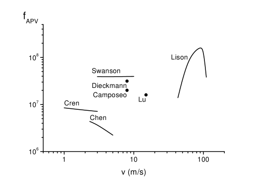
FIG. 2.: The quality factor $f_{APV}$ versus atomic longitudinal velocity for several alkali sources of cold atomic beams. Camposeo et al. [30] (Cs), Chen et al. [33] (Rb), Cren et al. [34] (Rb), Dieckmann et al. [35] (Rb), Swanson et al. [36] (Rb), Lison et al. [38] (Cs), Lu et al. [39] (Rb).

On Figure 2 we plot the quality factor versus the velocity for several beams of cold stable atoms chosen among those having a small spread of longitudinal velocities. The existing designs present themselves as grouped into three categories : the ultra-cold beams using a moving molasses [33, 34], the cold beams extracted from a 2D-MOT [30, 35, 36, 39] and the Zeeman-slowed device using a collimator [38]. In view of optimizing APV measurements on stable atoms, this last device is expected to lead to the best results, although the pyramidal trap remains of real interest due to its simplicity and probably better adaptability to radioactive isotopes. As we noted previously, the performances expected with the cold atomic beams are limited essentially by their divergence. However one may imagine two means of palliating this kind of difficulty.

i) Multiple passages of the excitation beam : it looks possible to widen the interaction region, at fixed density of excitation energy, by performing forward-backward passages of the beam between two spherical mirrors. The two mirrors should be pierced, one for providing the passage of the atomic beam at the output of the MOT and the other the passage of the counterpropagating excitation laser [43].

ii)Insertion of a collimator at the output of the MOT : It would seem very interesting to insert at the output of a two dimensional MOT a collimator similar to that described in [38]. Besides the beam collimation this device has the attractive feature of deflecting the atomic beam by a small angle, thus making possible to place the interaction region inside a Fabry-Perot cavity which provides enhancement of the excitation energy density. However we must be aware that a transverse temperature at the output of the collimator less than 50 $\mu$K looks difficult to achieve. Therefore the divergence of the slow beam remains well above that of the faster Zeeman-slowed beam.

III A well adapted observable physical quantity and two interaction regions

The choice of the observable physical quantity which manifests APV also plays an important role, since it determines the specific nature of the signal (absence or presence of a background), its signature and it also conditions the detection efficiency. In our first experiment in Paris [44], as well as in our current second-generation one [40], we have chosen to detect an angular momentum anisotropy in the excited state (either an atomic orientation in the first version, or an atomic alignment in the latter) providing a very specific signal without background. However, fluorescence detection efficiency of the 7S state orientation was low ($\sim 10^{-3}$), due to the need of polarization analysis on a single fine structure line. Alignment detection can be conducted efficiently using stimulated emission detection [40, 45]. However, in view of the very small number of atoms available in a trap, there is no possibility of signal amplification by the stimulated emission process advantageously used in a dense vapor. Therefore, with a cold beam there is a strong incentive for detecting the PV effect on the absorption rate.

We suggest to create a spin polarization $\vec{P}_{e}$ of the atomic beam at the output of the trap in a direction perpendicular to its velocity. Then, a specially well adapted observable physical quantity is a contribution to the absorption rate involving this spin polarization. It results from an interference between the parity-violating electric dipole amplitude $E_{1}^{pv}$ and the Stark amplitude induced by a transverse electric field. More precisely, the manifestation of APV would

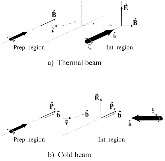
FIG. 3.: Schemes of the geometrical configurations relative a) to the Boulder experiment performed with a thermal atomic beam [2] and b) to the present proposal using a cold and slow atomic beam. Both exploit the spin polarization $\vec{P}_{e}$ of the atoms performed in a preparation region and use a transverse Stark electric field $\vec{E}$ in the interaction region. Both make use of a circularly polarized excitation beam (helicity $\xi$). With the thermal beam, the excitation beam has to be transverse to the velocity and the magnetic field $\vec{B}$, large enough to resolve the Zeeman components, has to rotate its direction by $\pi/2$ between the preparation and interaction regions, while with the cold beam the excitation can be longitudinal and only a small magnetic field $\vec{b}$, of uniform direction, is required, to preserve the spin polarization between the two regions. The pseudoscalar $\vec{E}\cdot\xi\hat{k}\wedge\vec{B}$ manifesting APV in case a) is replaced by $\vec{E}\cdot\xi\hat{k}\wedge\vec{P}_{e}$ in case b).

then rely on the presence in the absorption rate of the pseudoscalar quantity $\vec{E}\wedge\xi\hat{k}\cdot\vec{P}_{e}$, where $\xi\hat{k}$ represents the angular momentum of the light beam which excites the transition and $\vec{E}$ is the applied static electric field. It has the advantage of appearing in the total population of the excited state. It can be detected by monitoring the total intensity of the fluorescence light emitted during the two-step desexcitation process, involving either the $6P_{1/2}$ or the $6P_{3/2}$ state. No polarization analysis nor even light filtering (except for stray light) is necessary in principle. The APV signal is odd under the separate reversals of the electric field, the spin polarization and the helicity of the photons which excite the transition. We relegate to the appendix the derivation of the signal expression in the most general conditions. Here we present the result in the particular case of ¹³³Cs (I=7/2), for the experimental configuration shown in Fig. 4, supposing no magnetic field and a total circular polarization of the excitation beam, $\xi=2\,{\rm Im}\{\epsilon_{x}^{*}\epsilon_{y}\}=\pm 1$ (hence $|\hat{\epsilon}\cdot\hat{u}\,|^{2}=1/2$ whatever $\hat{u}\perp\hat{k}$ ).

$$N_{7S}\propto\beta^{2}E^{2}-\frac{3}{4}\;(M^{\prime}_{1}+\xi\;{\rm Im}E_{1}^{pv})\;\beta\vec{E}\wedge\hat{k}\cdot\vec{P}_{e}\hskip 28.45274pt{\rm for\;the}\;\;6S,F=3\rightarrow 7S,F=4\;\;{\rm line}\;,$$ (1)

$$N_{7S}\propto\beta^{2}E^{2}-\frac{5}{4}\;(M^{\prime}_{1}+\xi\;{\rm Im}E_{1}^{pv})\;\beta\vec{E}\wedge\hat{k}\cdot\vec{P}_{e}\hskip 28.45274pt{\rm for\;the}\;\;6S,F=4\rightarrow 7S,F=3\;\;{\rm line}\;.$$ (2)

$\beta$ denotes the vector polarizability of the transition and $M^{\prime}_{1}$, the magnetic dipole amplitude, which is the sum of the many-body contribution $M_{1}$ and that induced by the hyperfine interaction $M_{1}^{hf}$. Here we assume the applied electric field large enough so that the field-independent contribution proportional to $M_{1}^{\,{}^{\prime}2}$ can be neglected.

We note that this circular dichroism of a transversally polarized sample, $\vec{E}\cdot\xi\hat{k}\wedge\vec{P}_{e}$, could not be envisaged in a dense vapor where the spin polarization is rapidly destroyed by collisions. By contrast, (co-)counter-propagation of the atomic and light beams provides the attractive possibility of having both beams passing through two interaction regions leading to circular dichroism of opposite sign. For instance, one can choose two orthogonal directions of $\vec{E}$ in these two regions, with the direction of $\vec{P}_{e}$ taken at $\pm 45^{\circ}$ to the direction of $\vec{E}$ in one and the other region (See configurations 1 and 2, or 3 and 4, represented in Fig. 4). Then, the difference of fluorescence rates in those two regions can selectively provide the $\vec{P}_{e}$-dependent contribution of interest. In the next section, we shall show that such a differential measurement also offers the important additional advantage of suppressing some dangerous systematic effects.

It is important to notice that real time calibration of the PV signal is easy to obtain. By selecting in the fluorescence rate the contribution odd under the separate reversals of the electric field and the spin polarization, but even in the reversal of the light helicity, we can isolate the $M^{\prime}_{1}$-Stark interference signal. Thereby the amplitude ${\rm Im}E_{1}^{pv}$ is directly calibrated in terms of $M^{\prime}_{1}$. If one reminds that $M^{\prime}_{1}=M_{1}\pm M_{1}^{hf}$, depending on the hyperfine transition $\Delta F=\pm 1$, we see that absolute calibration of ${\rm Im}E_{1}^{pv}$ in terms of the theoretically well known amplitude $M_{1}^{hf}$ is possible.

Another observable physical quantity appearing in the absorption rate has been proposed in [47]. It does not require any spin polarization of the ground state, but it involves the application of a magnetic field $\vec{B}$, transverse to the light beam, which enters explicitly into the definition of the pseudoscalar manifesting parity violation, $\vec{E}\cdot\xi\hat{k}\wedge\vec{B}$. However, for observing this effect the field has to be large enough for the Zeeman components to be resolved, otherwise compensations occur [48]. This is, actually, the APV effect which has been detected by the Boulder group [49]. In the most recent version of their experiment [2] (see Fig. 3-a for a schematic representation of the configuration), the atomic beam is spin polarized in a preparation zone before entering the interaction region, but a magnetic field (6.4 G), whose purpose is to resolve the Zeeman lines is still applied, although the atomic spin polarization prepared in the ground state makes this unnecessary, as Eq. 1 shows. With the same set-up, a much weaker field would be sufficient for preserving the direction of the atomic orientation between the preparation and the interaction regions. This would avoid slight line overlap of adjacent Zeeman lines and the associated difficulties.

We, now, want to comment about the conditions to be fulfilled by the magnetic field, which obviously cannot be perfectly cancelled. There are strict requirements: the magnetic field of the MOT has to be screened. Instead, a small $\vec{B}$ field along the direction wanted for the spin polarization is needed in the optical pumping region as well as in the two interaction regions and, consequently, in between those two regions: otherwise the rapid spin precession might result in spin disorientation (when the spins do not follow adiabatically the field direction). Finally, the exact direction of $\vec{P}_{e}$ inside the interaction regions, involved in the pseudoscalar manifesting APV, is actually determined by the $\vec{b}$ field direction in those regions, eventhough this field (typically 100 mG) is small enough to avoid broadening of the transition. We note that those conditions are easier to fulfill than those realized in [2], since the field direction remains the same between the preparation and the interaction regions (see Fig. 2), instead of having to be rotated by $\pi/2$.

IV Suppression of the systematic effect arising from the $M^{\prime}_{1}$ Stark interference via optical birefringences

As we may note on Eq. 1, when the sign of the true scalar $\vec{P}_{e}\cdot\vec{E}\wedge\hat{k}$ is reversed, the discrimination between the $E_{1}^{pv}$-Stark and the $M^{\prime}_{1}$-Stark interference signals hinges on their opposite behaviour under reversal of the pseudoscalar $\xi$, the excitation light helicity. Since in ¹³³Cs, the latter is the larger of the two signals, by a factor $2\times 10^{4}$, this is a major source of potential systematic effect. Indeed, APV measurements previously performed in a transverse electric field have all met the difficulty associated with the presence of the parity conserving interference effect, which can mimic the PV signal if the reversal of the light helicity $\xi$ is imperfect, i.e. if a small component of linear polarization changes its sign simultaneously with $\xi$. This kind of problem occurs when the optics on the path of the excitation beam possess some birefringence, a defect difficult to avoid completely at the level required.

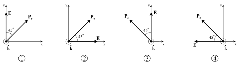
FIG. 4.: The four geometrical configurations considered in the text, specified by the relative directions of the Stark field, $\vec{E}$, the spin polarization created in the ground state, $\vec{P}_{e}$, and the wave vector of the excitation laser $\hat{k}$; $\xi$ is assumed the same in the four configurations; the atom velocity is along $\hat{k}$, orthogonal to the page. By combining measurements performed in those four configurations, the PV signal is obtained with considerable reduction of the systematic effect arising from the $M^{\prime}_{1}$-Stark interference signal via optical birefringences.

For the complete discussion given below, we have to write down the expression for the $M^{\prime}_{1}$-Stark signal assuming the most general description of the excitation light polarization. It is expressed in terms of the four Stokes parameters, which give a general representation of the beam polarization properties: $u_{0}=|\epsilon_{y}|^{2}$ + $|\epsilon_{x}|^{2}$; $u_{1}={\rm Re}\{\epsilon_{x}\epsilon_{y}^{*}+\epsilon_{x}^{*}\epsilon_{y}\}$; $u_{2}\equiv\xi={\rm Im}\{\epsilon_{x}^{*}\epsilon_{y}-\epsilon_{x}\epsilon_{y}^{*}\}$; $u_{3}=|\epsilon_{y}|^{2}$ - $|\epsilon_{x}|^{2}$. The first parameter $u_{0}$ represents the unpolarized intensity. If it is normalized to unity, the other parameters represent polarization ratios measured by a linear analyzer directed along x, then y ($u_{3}$) or along the bisectors of x and y ($u_{1}$) or by a direct then inverse circular analyzer ($u_{2}$).

According to Eq. 19 of Appendix A, the general expression for the $M^{\prime}_{1}$-Stark interference signal ${\cal S}(M_{1})$ is given by:

$${\cal S}(M_{1})=-2M^{\prime}_{1}\,{\rm Re}\{(\beta\vec{E}\wedge\hat{k}\cdot\hat{\epsilon})(\hat{\epsilon}^{*}\cdot\vec{P}_{e})\}\,.$$ (3)

We consider the four distinct geometrical configurations represented on Fig.4. Measurements relative to configurations 1 and 2 (or 3 and 4) can be performed simultaneously in the two distinct interaction regions, whereas reversal of $\vec{P}_{e}$ by $\pi/2$ is needed for changing configuration 1 into 3 and 2 into 4. It is interesting to compare the ${\cal S}(M_{1})$ signals expected in those four configurations:

$${\cal S}_{1}(M_{1})=-2M^{\prime}_{1}\beta E\left(|\epsilon_{x}|^{2}+{\rm Re}\{{\epsilon_{x}^{*}\epsilon_{y}\}}\right)=-M^{\prime}_{1}\beta E\left(u_{0}-u_{3}+u_{1}\right)$$ (4)

$${\cal S}_{2}(M_{1})=\;\;\,2M^{\prime}_{1}\beta E\left(|\epsilon_{y}|^{2}+{\rm Re}\{{\epsilon_{x}^{*}\epsilon_{y}\}}\right)=\;\;\,M^{\prime}_{1}\beta E\left(u_{0}+u_{3}+u_{1}\right)$$ (5)

$${\cal S}_{3}(M_{1})=\;\;\,2M^{\prime}_{1}\beta E\left(|\epsilon_{x}|^{2}-{\rm Re}\{{\epsilon_{x}^{*}\epsilon_{y}\}}\right)=\;\;\,M^{\prime}_{1}\beta E\left(u_{0}-u_{3}-u_{1}\right)$$ (6)

$${\cal S}_{4}(M_{1})=-2M^{\prime}_{1}\beta E\left(|\epsilon_{y}|^{2}-{\rm Re}\{{\epsilon_{x}^{*}\epsilon_{y}\}}\right)=-M^{\prime}_{1}\beta E\left(u_{0}+u_{3}-u_{1}\right)$$ (7)

On the other hand configurations 1 and 2 provide opposite circular dichroism i.e. opposite PV signals, ${\cal S}_{1}(PV)=-{\cal S}_{2}(PV)=\left({\rm Im}E_{1}^{pv}\beta\vec{E}\wedge\xi\hat{k}\cdot\vec{P}_{e}\;\right)$, and the same result holds for 3 and 4. From the above set of four equations one can form the linear combination

$${\cal S}_{1}-{\cal S}_{2}-{\cal S}_{3}+{\cal S}_{4}=4\left({\,\cal S}_{1}(PV)-M^{\prime}_{1}\,\beta E\,u_{0}\;\right)\,,$$ (8)

which shows up an important property : the contribution of the $M^{\prime}_{1}$-Stark interference signal involves only the unpolarized intensity, $u_{0}$. Thereby when $\xi$ is reversed, so as to isolate the $E_{1}^{pv}$ contribution, we reduce considerably the risk which would have come from $\xi-odd$-contributions contaminating either $u_{3}$ or $u_{1}$, via the birefringence of the optics.

As a convenient and reliable means of performing helicity reversal, one can use the polarization modulator described in ref [51]. It provides specific labelings of the three Stokes parameters, $u_{1},\;\xi\equiv u_{2}$, and $u_{3}$, by distinct modulations. In this way both signals ${\cal S}(PV)$ and ${\cal S}(M_{1})$ appearing at different frequencies are detected by synchronous detection.

Additional discrimination of ${\cal S}(PV)$ against ${\cal S}(M_{1})$, respectively even and odd under $\hat{k}$ reversal, can be obtained by performing multiple passages of the beam between two mirrors pierced in their center, following a procedure used in [43, 44].

V Magnitude of the expected signals

In the preceding sections we have made precise suggestions for adapting APV measurements to a source of cold atoms. Now, we intend to give an estimate of both the APV and the $M^{\prime}_{1}$-Stark interference signals, ${\cal S}(PV)$ and ${\cal S}(M_{1})$, and their Signal to Noise ratios (SNR), assuming reasonable magnitudes of the Stark field and the laser intensity. We note that the shot noise limited SNR is independent of the magnitude of the Stark field. We take the example of ¹³³Cs in order to make easier comparison with other atomic sources already exploited. First, we need to evaluate the excitation probability per unit of time: ${\cal R}_{ex}=\frac{dN_{Cs}^{*}}{dt}/N_{Cs}=\sigma_{ex}(E)\times\Phi_{ex}$, where $\Phi_{ex}$ is the flux of excitation photons. The excitation cross section without electric field, $\sigma_{nat}=\sigma_{ex}(E=0)$, without Doppler broadening, for an isotope without nuclear spin, excited by a single-mode laser centered in frequency at the transition peak, is given in ref [41]:

$$\sigma_{nat}=\frac{\lambda^{2}}{2\pi}\;\frac{\Gamma_{M^{\prime}_{1}}}{\Gamma_{7S}}=2.45\times 10^{-23}\;{\rm cm}^{2}\,.$$ (9)

Here ${\Gamma_{7S}}$ denotes the natural width of the 7S state and $\Gamma_{M^{\prime}_{1}}$ the partial width associated with the $M^{\prime}_{1}$ amplitude. Assuming excitation of the $6S_{F}\rightarrow 7S_{F^{\prime}}$ line in an electric field, using the results of Appendix A, we obtain:

$$\sigma_{ex}(E)=\frac{(2F^{\prime}+1)}{2(2I+1)}\times\frac{2}{3}(1-g_{{}_{F^{\prime}}})\times\left(\frac{\beta E}{M^{\prime}_{1}}\right)^{2}\sigma_{nat}$$ (10)

A Measurement of $M^{\prime}_{1}/\beta E$ with a cold atomic beam (proposal 1)

For a Stark electric field of 1000 V/cm, leading to $\sigma_{ex}(E)=0.89\times 10^{-20}$ cm² for the $6S_{F=3}\rightarrow 7S_{F^{\prime}=4}$ line and $\beta E/M_{1}=1000/30$, for an excitation beam of waist radius 1 mm, delivering 500 mW at 539.4 nm ($\Phi_{ex}$ = 0.95 $\times 10^{20}$ photons s^-1/cm²), we predict ${\cal R}_{ex}=0.89\times 10^{-20}\times 0.95\times 10^{20}=0.84$ s^-1. Using the number of Cs atoms in the interaction region, given in Table 1 (proposal 1), we expect $\frac{dN^{*}_{Cs}}{dt}=0.84\times 10^{7}$s^-1 for the two interaction regions, each 20 mm long. Supposing a fluorescence detection efficiency of 10 $\%$, we predict a collected fluorescence rate of $\sim 10^{6}$ s^-1. Using Eq. 1 (and 2), with $|\vec{E}\cdot\hat{k}\wedge\vec{P}_{e}|=1/\sqrt{2}$, we expect a SNR$\simeq 15/\sqrt{\rm Hz}$ for ${\cal S}(M_{1})$ for the $6S_{F=3}\rightarrow 7S_{F^{\prime}=4}$ line (and $\simeq 20/\sqrt{\rm Hz}$ on the $6S_{F=4}\rightarrow 7S_{F^{\prime}=3}$ line). Hence a statistical precision of $10^{-3}$ can be obtained with an integration time of about one hour. For the measurement of $M_{1}^{hf}\sim M^{\prime}_{1}/5$ at the same level of precision, the integration time has to be 25 times longer, for both $\Delta F=1$ and $-1$ lines. This looks possible to achieve. We believe that the conditions for observing this signal could be made excellent : thanks to the very good vacuum realized by differential pumping in the beam compartment which is well separated from the MOT by the pyramidal assembly, we can expect nearly no background. In this respect the signature given to ${\cal S}(M_{1})$ by modulating $u_{3}$ and $u_{1}$ (see Eqs 4 to 7) should be of great help.

On the other hand, with ${\rm Im}E_{1}^{pv}/\beta E=1.6\times 10^{-6}$, there is no chance to achieve APV measurements without recourse to some amplification process. A possibility might rely on multiple passages of the excitation beam which can also provide efficient suppression of the $M^{\prime}_{1}$-Stark interference signal and hence further reduction of the associated systematics. If we denote by $\kappa$ the signal enhancement factor, the SNR for ${\cal S}(PV)$ becomes $\sim\sqrt{\kappa}\times 10^{-3}/\sqrt{\rm Hz}$, hence the time required for observing the PV effect with SNR = 1 is $10^{6}/\kappa$ seconds. An enhancement factor larger than 100 would be necessary for obtaining worthwhile conditions of measurement.

We can now examine the situation with francium. As mentioned earlier we can expect the francium $M^{\prime}_{1}$ amplitude to be one order of magnitude larger than the cesium one. This increases the ${\cal S}(M_{1})$ without adding noise. The shot noise limited SNR ratio is thus increased by a factor of 10. On the other hand, the atom flux will certainly be reduced. The best production rates of Fr⁺ ions available in the world is, to our knowledge, at the ISOLDE facility at CERN : it amounts to $\sim 10^{9}$ s^-1. We are presently uncertain about the efficiency of neutralization and collection in the MOT, $\zeta$, one may expect. A fairly conservative estimate might be $\zeta\sim 10^{-2}$. However, taking into account that a 80$\%$ ion to atom conversion efficiency has been reported for the converter used on-line at ISOLDE [52] and that a 16$\%$ collection and trapping efficiency has been achieved with Fr atoms [39], we can reasonably hope that $\zeta\approx 0.1$ is achievable. The SNR is reduced by $\sqrt{\zeta}$. All in all, we can consider that not only does the observation of the forbidden 7S-8S transition look feasible but so too does a measurement of its magnetic dipole amplitude with an accuracy better than 10$\%$. This would provide an important test of atomic models [12]. Such an experiment would also give invaluable insight into how to perform a future measurement of $Q_{W}({\rm Fr})$ : for such a measurement to become possible with an efficiency $\zeta=10^{-2}$, the same enhancement factor $\kappa=100$ as for cesium is required.

B Prospect for APV observation with an ultra cold atomic beam (proposal 2)

As shown in Table I, the ultra cold beam can a priori offer better performances owing to the possibility of lengthening the interaction time. However, this advantage is spoiled by the effect of the beam divergence, which one would like to reduce by a factor of $\sim 3$. One possibility consists in making additional transverse cooling of the atomic beam simultaneously at the output of the MM-MOT, using an auxiliary 2D MOT according to a scheme used by the authors of ref[34] for loading the beam into a magnetic guide. If one wants to benefit from the lowest velocities, $\sim$ 20 cm/s reported in[34], a priori very interesting here, one has to solve the problem of collisional losses of the slow atomic beam with atoms in the vapor cell on its way to the interaction region, possibly by using other means for loading the trap.

Another important technical question, beyond the scope of the present paper, concerns the possibility of combining the advantages of multiple passages of the longitudinal excitation beam with those of the ultra-cold atomic beam.

C APV observation with a Zeeman-slowed atomic beam (proposal 3)

The number of atoms in the interaction region obtainable with the Zeeman slower is given in table I. It corresponds to a gain by a factor of $\sqrt{17}$ with respect to the slow and cold atomic beam (proposal 1). The shot noise limited S/N ratio for ${\cal S}(PV)$, increased by that same factor, becomes $\sqrt{17\kappa}\times 10^{-3}/\sqrt{\rm Hz}$. For becoming competitive with the thermal beam Boulder experiment, from the sole point of view of SNR ratio, an enhancement factor $\kappa$ of $\sim 6\times 10^{3}$ is necessary. In this experiment, the collimator causes a deflection of the atomic beam and a Fabry-Perot cavity enhancing the intensity of the excitation beam all along the interaction region does not look too unrealistic, but the enhancement factor required for obtaining the same SNR is comparable to that achieved in Boulder. One may, however, expect that the high power stored inside the cavity will have here somewhat milder drawbacks. Indeed, longitudinal excitation allows to all the excited atoms to explore the interference pattern over several wavelengths during their lifetime, hence the difficulty associated with inhomogeneous light shifts causing asymmetric line shapes should be suppressed. In conclusion, for APV measurements on the stable ${}^{133}Cs$ atom the Zeeman slower is an interesting possibility but, with respect to the thermal beam [2], we cannot expect neither simplifications of the set-up, nor drastic improvement of the SNR ratio.

VI Conclusion

In this paper we have addressed the question of how to best use a cold atom source for performing APV measurements. For fighting against the large drawback associated with the small number of atoms compared with cells, one must take the maximum advantage of their narrow velocity distribution. This advantage makes it possible to excite a beam of slow and cold atoms by a (co-)antico-linear laser, spatially matching the atomic beam over several centimeters, without any Doppler broadening. With respect to a thermal beam, the lengthening of the interaction time thus achieved ranges between $10^{3}$ and $10^{4}$. On the other hand, we have made a new proposal concerning the observable physical quantity manifesting APV. The atomic beam should be given a transverse spin polarization, $\vec{P}_{e}$. The new observable reflects existence of a circular dichroism. It involves the pseudoscalar $\vec{E}\cdot\xi\hat{k}\wedge\vec{P}_{e}$ and appears in the population of the upper state, hence in the total fluorescence light. Therefore fluorescence detection efficiency is a crucial parameter to be optimized. Moreover, with two interaction regions leading to opposite circular dichroism, it is possible to make differential measurements. If, in addition, the spin polarization $\vec{P}_{e}$ can be sequentially rotated by $\pi/2$, then by combining the four results obtained in the two interaction regions for the two orientations of $\vec{P}_{e}$, it is also possible to achieve important reduction of the systematic effects that birefringence of the optics may generate from the $10^{4}$ times larger $M_{1}$-Stark interference signal.

The merit of cold atom sources relies on their potential to localize atoms, only one of the conditions required to extend APV measurements in the long term to radioactive isotopes. Suppression of Doppler broadening and lengthening of the interaction time are other important benefits. However, our estimate of the S/N ratio shows that, in the present state of the art, those do not appear sufficient to solve the difficulty of precise APV measurements. Nevertheless, exploratory experiments performed on stable alkali highly forbidden transitions, can provide a valuable step enabling us to define the beam specifications required for APV experiments with radioactive isotopes. We have shown that by combining experimental techniques proven elsewhere, there is a reasonable hope of observing the 6S-7S transition for ¹³³Cs and of making a $10^{-3}$ accurate measurement of $M_{1}^{hf}/\beta$ with a beam of slow, cold atoms with an unsophisticated set-up. Furthermore, such an experiment could be considered as a prototype to evaluate the production rate of Fr atoms needed to extend such measurements from stable ¹³³Cs to radioactive Fr. With a Zeeman slower providing a monokinetic beam of high flux and low divergence, PV measurements on ¹³³Cs as precise as those presently existing do not look impossible, but a real progress with respect to a thermal beam does not look obvious to us. We hope that our present contribution will stimulate both reflections and experimental work towards advances in this emerging field of research.

We thank particularly D. Guéry-Odelin, L. Moi, C. J. Foot, D. Cassettari, A. Camposeo and F. Cervelli for very stimulating discussions and practical advice for preparing the ongoing construction of a laser trap. We are grateful to M.D. Plimmer for critical reading of the manuscript. A.W. acknowledges support from CNRS (IN2P3) and S.S. from the European Commission.

^a Also at E. Fermi Physics Dept., Pisa Univ., Pisa, Italy.

References

Appendix A

We are now going to present the derivation of the population signal in the experimental configuration specified in this paper. The nS, F $\rightarrow$ (n+1)S, F’ transition amplitudes can be obtained from the effective transition matrix $T$ acting on the electronic spin states of the form:

$$T=a1{\rm I}+\vec{b}\cdot\vec{\sigma}$$ (11)

$1{\rm I}$ is the two-by-two unit matrix and the components of $\vec{\sigma}$ are the three Pauli matrices. The parameters $a$ and $\vec{b}$ are given by:

$$a = \alpha\vec{\rm E}\cdot\hat{\epsilon}$$ (12)

$$\vec{b} = i\beta\;{\rm\vec{E}}\wedge\hat{\epsilon}-M^{\prime}_{1}\hat{k}\wedge\hat{\epsilon}+i{\rm Im}E_{1}^{pv}\hat{\epsilon}\;.$$ (13)

where $\alpha$ and $\beta$ are the scalar and vector transition polarizabilities, $M^{\prime}_{1}$ and $E_{1}^{pv}$ are the magnetic dipole and the parity-violating electric dipole transition amplitudes, and $\hat{\epsilon}$ represents the laser polarization.

In the present situation, stimulated emission is totally negligible compared with spontaneous emission and optical coherences between the two S states can be ignored. We assume that the laser selects one hfs component nS, F $\rightarrow$ (n+1)S, F’. The excited state density matrix, up to a normalization factor, is then given by:

$$\rho=P_{{}_{F^{\prime}}}\,TP_{{}_{F}}\,\rho_{g}P_{{}_{F}}\,T^{\dagger}\,P_{{}_{F^{\prime}}}\,,$$ (14)

where $\rho_{g}$ is the restriction of the density operator to the nS ground state. $P_{{}_{F}}$ is the projector on the nS, F sublevel and $P_{F^{\prime}}$ the projector on the (n+1)S, F’ sublevel. We assume an electronic orientation, $\vec{P}_{e}$, has been created in the ground state:

$$\rho_{g}=1{\rm I}+\vec{P}_{e}\cdot\vec{\sigma}\,.$$ (15)

This definition implies that : ${\rm Tr}\rho_{g}=2(2I+1)$. Therefore, a common normalization factor 1/2(2I+1) has to be applied to all the quantities computed below. It is taken into account in Eq. 10.

In order to compute the 7S population and its spin polarization, proportional respectively to Tr $\rho$ and Tr $\rho\vec{\sigma}$, we apply the Wigner-Eckart theorem to the spin operator $\vec{\sigma}$ acting in the hyperfine subspace F :

$$P_{{}_{F}}\,\vec{\sigma}P_{{}_{F}}=2g_{{}_{F}}\,P_{{}_{F}}\,\vec{F},\hskip 28.45274pt{\rm where}\hskip 14.22636ptg_{{}_{F}}=2(F-I)/(2I+1).$$ (16)

Using Eqs 1 to 6 we obtain for the $\Delta F=F^{\prime}-F$ transition:

$${\rm Tr}\rho=n_{{}_{F^{\prime}}}(\delta_{{}_{FF^{\prime}}}aa^{*}+h_{{}_{FF^{\prime}}}\,\vec{b}\cdot\vec{b}^{*})+[n_{{}_{F^{\prime}}}p_{{}_{F^{\prime}}}\delta_{{}_{FF^{\prime}}}(a\vec{b}^{*}+a^{*}\vec{b}\,)-n_{{}_{F}}p_{{}_{F}}g_{{}_{F^{\prime}F}}i\vec{b}\wedge\vec{b}^{*}]\cdot\vec{P}_{e}\,,$$ (17)

$${\rm Tr}\rho\vec{\sigma}=n_{{}_{F^{\prime}}}p_{{}_{F^{\prime}}}[\delta_{{}_{FF^{\prime}}}(a\vec{b}^{*}+a^{*}\vec{b}\,)+g_{{}_{FF^{\prime}}}i\vec{b}\wedge\vec{b}^{*}]+\vec{P}_{e}\;{\rm-dependent\;contributions}\,,$$ (18)

where $n_{{}_{F^{\prime}}}=2F^{\prime}+1,\;p_{{}_{F^{\prime}}}=(1+2g_{{}_{F^{\prime}}})/3,\;$ and,

if $\Delta F=0,h_{{}_{FF^{\prime}}}=p_{{}_{F^{\prime}}}$, and $g_{{}_{FF^{\prime}}}=g_{{}_{F^{\prime}}}$;

if $\Delta F=\pm 1,h_{{}_{FF^{\prime}}}=2(1-g_{{}_{F^{\prime}}})/3\equiv 4g_{{}_{F}}^{2}F(F+1)/3$ and $g_{{}_{FF^{\prime}}}=1-g_{{}_{F^{\prime}}}$.

The second term in the RHS of Eq. 17 represents the contribution to the upper state population which depends on the initial state orientation $\vec{P}_{e}$, while Eq. 18 gives the orientation of the upper state created by the excitation process, the observable physical quantity that we detected in our first APV experiment [44]. We note the close connection between those two contributions in which the role of the initial and final states is interchanged. (Note the appearance of F, and not F’, in the last term of the RHS of Eq. 17).

Keeping only the terms which depend on the Stark field, we obtain for a $\Delta F=\pm 1$, nS, F $\rightarrow$ (n+1)S, F’, transition:

$${\rm Tr}\rho=(2F+1)\frac{1-g_{{}_{F}}}{3}\times$$ (19)

$$\left[2\beta^{2}|\vec{E}\wedge\hat{\epsilon}|^{2}-(1+2g_{{}_{F}})\left({\rm Im}E_{1}^{pv}\beta\vec{E}\wedge\xi\hat{k}\cdot\vec{P}_{e}+2M^{\prime}_{1}{\rm Re}\{(\beta\vec{E}\wedge\hat{k}\cdot\hat{\epsilon})(\hat{\epsilon}^{*}\cdot\vec{P}_{e})\}+\beta^{2}\xi(\vec{E}\cdot\hat{k})(\vec{E}\cdot\vec{P}_{e})\right)\right]\;.$$ (20)

The last $\vec{P}_{e}$-dependent contribution in Eq. 19 vanishes when there is no longitudinal component of the electric field.

References

- [1] M. A. Bouchiat and C. Bouchiat, J. Phys. France, 35, 899 (1974) and Rep. Prog. Phys. 60, 1351 (1997).
- [2] C. S. Wood, et al, Science, 275, 1759 (1997).
- [3] S. C. Bennett and C. E. Wieman, Phys. Rev. Lett. 82, 2484 (1999).
- [4] V. A. Dzuba, V. V. Flambaum and O. P. Sushkov, Phys. Lett. A 141, 147 (1989); and 142, 373 (1989); S. A. Blundell, W. R. Johnson and J. Sapirstein, Phys. Rev. Lett. 65 1411 (1990) ; Phys. Rev. D 45, 1602 (1992).
- [5] A. Derevianko, Phys. Rev. Lett. 85, 1618 (2000).
- [6] A.I. Milstein, O.P. Sushkov, I.S. Terekhov, Phys. Rev. Lett 89, 283003 (2002).
- [7] V. A. Dzuba, V. V. Flambaum, J. S. M. Ginges, Phys Rev. D 66 076013 (2002); M. Yu. Kuchiev and V.V. Flambaum, Phys. Rev. Lett 89, 283002 (2002).
- [8] D. DeMille, Phys. Rev. Lett. 74, 4165 (1995).
- [9] A.-T. Nguyen, D.E. Brown, D. Budker, D. DeMille, D.F. Kimball, and M. Zolotorev, in ”Parity Violation in Atoms and Electron Scattering”, B. Frois and M. A. Bouchiat, eds., World Scientific, 1999, p. 295; A.-T. Nguyen, D. Budker, D. DeMille, and M. Zolotorev, Phys. Rev. A 56, 3453 (1997).
- [10] V. A. Dzuba,V. V. Flambaum, O. P. Sushkov, Phys. Rev. A 51, 3454 (1995).
- [11] Y. B. Zel’dovich, Sov. Phys. JETP 6, 1184 (1957); V. V. Flambaum and I. B. Khriplovich, Sov. Phys. JETP 52, 835 (1980); C. Bouchiat and C. A. Piketty, Z. Phys. C, 49, 49 (1991).
- [12] I. M. Savukov, A. Derevianko, H. G. Berry, W. R. Johnson, Phys. Rev. Lett. 83, 2914 (1999).
- [13] H. J. Metcalf and P. Van der Straten, in Laser cooling and trapping of atoms, Springer, New-York (1999).
- [14] S. N. Atutov et al., Phys. Rev. A 60, 4693 (1999).
- [15] Z-T. Lu et al., Phys. Rev. Lett. 72 , 3791 (1994).
- [16] J. A. Behr et al., Phys. Rev. Lett. 79 , 375 (1997).
- [17] G. Gwinner et al., Phys. Rev. Lett. 72 , 3795 (1994).
- [18] M. D. Di-Rosa, S. G. Crane, J. J. Kitten, W. A. Taylor, D. Vieira, X. Zhao, SPIE-Int. Soc. Opt. Eng. 34-45, 4634 (2002).
- [19] J. E. Simsarian et al., Phys. Rev. Lett. 76 , 3522 (1996).
- [20] Z-T. Lu et al., Phys. Rev. Lett. 79 , 994 (1997).
- [21] J.S. Grossman, L.A. Orozco, M. R. Pearson, G. D. Sprouse, Physica Scripta, TIE1, 1 (2000).
- [22] M. A. Bouchiat and J. Guéna, J. Phys. France 49, 2037 (1988); C. Bouchiat and C. A. Piketty, J. Phys. France, 49, 1851 (1988).
- [23] W.R. Johnson, Phys. Rev. A 60, R1741 (1999); V. A. Dzuba, V. V. Flambaum, Phys. Rev. A 62, 052101 (2000).
- [24] A.A. Vasilyev, I.M. Savukov, M.S. Safronova and H.G. Berry, Phys. Rev. A 66, 020101 (2002).
- [25] R. Casalbuoni et al., Phys. Lett. B 460, 135 (1999); J. Erler and P. Langacker, Phys. Rev. Lett. 84, 212 (2000); D.E. Groom, http://pdg.lbl.gov/ (ch.10).
- [26] J. E. Simsarian, W. Z. Zhao, L. A. Orozco, and G. D. Sprouse, Phys. Rev. A 59, 195 (1999).
-
[27]
See for example: S. Chu, Rev. Mod. Phys. 70, 685 (1998);
C. N. Cohen-Tannoudji, Rev. Mod. Phys. 70, 707 (1998);
W. D. Phillips, Rev. Mod. Phys. 70, 721 (1998). - [28] K. I. Lee, J.A. Kim, H. R. Noh, W. Jhe, Opt. Lett. 21 1177 (1996).
- [29] J. J. Arlt et al., Opt.Commun. 157, 303 (1998).
- [30] A. Camposeo et al., Opt.Commun. 200, 231 (2001).
- [31] M. A. Bouchiat, J. Guéna, and L. Pottier, J. Physique Lett. 45, 523 (1984).
- [32] E. Biémont, P. Quinet, and V. Van Renterghem, 31 5301 (1998).
- [33] H. Chen and E. Riis, Appl. Phys. B 70, 665 (2000)
- [34] P. Cren, C.F. Roos, A. Aclan, J. Dalibard, D. Guéry-Odelin, Eur. Phys. J. D 20, 107 (2002).
- [35] K. Dieckmann, R.J.C. Spreeuw, M. Weidemüller, J. T. M. Walraven, Phys. Rev. A 58, 3891 (1998).
- [36] T. B. Swanson, N. J. Silva, S. K. Mayer, J. J. Maki, D. H. McIntyre, J. Opt. Soc. Am. B 13, 1833 (1996).
- [37] J. Schoser et al., Phys. Rev. A 66, 023410 (2002).
- [38] F. Lison, P. Schuh, D. Haubrich, D. Meschede, Phys. Rev. A 61, 013405 (1999).
- [39] Z. T. Lu et al., Phys. Rev. Lett. 77, 3331 (1996).
- [40] J. Guéna et al., e-print physics/0210069, to appear in Phys. Rev. Lett.
- [41] M. A. Bouchiat and C. Bouchiat, J. Phys. France, 36, 493 (1975).
- [42] C.S. Wood et al., Can. J. Phys. 77, 7 (1999); B.P. Masterson et al., Phys. Rev. A, 47, 2139 (1993).
- [43] D. Herriott, H. Kogelnik, R. Kompfner, Appl. Opt., 3, 523 (1964); M. A. Bouchiat and L. Pottier, Appl. Phys. B 29, 43 (1982).
- [44] M. A. Bouchiat, J. Guéna, L. Hunter and L. Pottier, Phys. Lett. B 117, 358 (1982); ibid B 134, 463 (1984); J. Phys. (France) 47, 1709 (1986).
- [45] D. Chauvat, et al., J. Guéna, Ph. Jacquier, M. Lintz, and M. A. Bouchiat, Eur. Phys. J. D 1, 169 (1998); M. A. Bouchiat and C. Bouchiat, Z. Phys. D 36, 105 (1996).
- [46] V. A. Dzuba, V. V. Flambaum, J. S. M. Ginges, Phys. Rev. A 63, 062101 (2001).
- [47] M. A. Bouchiat and L. Pottier in Proceedings of the International Workshop on Neutral Current Interactions in Atoms, W. L. Williams and M. A. Bouchiat Ed. (Univ. of Michigan Press, Ann Arbor, 1979), p. 122, and Science 234, 1203 (1986).
- [48] M. A. Bouchiat, M. Poirier, C. Bouchiat, J. Physique (Paris) 40, 1127 (1979).
- [49] S. L. Gilbert and C.E. Wieman, Phys. Rev. A 34, 792 (1986).
- [50] M. A. Bouchiat, Ph. Jacquier, M. Lintz, L. Pottier, Opt.Commun. 56, 100 (1985).
- [51] M. A. Bouchiat and L. Pottier, Opt.Commun. 37, 229 (1981).
- [52] F. Touchard, et al., Nucl. Instr. and Meth. 186, 329 (1981).