Transient growth and instability in rotating boundary layers

Abstract

The three-dimensional temporal instability of rotating boundary layer flows is investigated by computing classical normal modes as well as by evaluating the transient growth of optimal disturbances. The flows examined are the rotating Blasius (RB) and the rotating asymptotic suction layers (RAS), with the rotation axis normal to the basic flow plane. In agreement with an inviscid criterion, streamwise unstable modes are found in both flow cases for anti-cyclonic rotation: at high Reynolds numbers, one obtains the Rossby number unstable range $0<1/{\rm Ro}<0.57$ for RB, or $0<1/{\rm Ro}<1$ for RAS. Critical Reynolds and Rossby numbers are also determined in both instances. Moreover the dependence of transient growth with respect to wavenumbers, Rossby and Reynolds numbers is presented for both cyclonic and anti-cyclonic régimes. In particular, the peak transient growth is computed for a wide range of parameter values within the cyclonic regime and is shown to be reduced by rotation. A scaling analysis with respect to the Reynolds number is performed showing that the standard ${\rm Re}^{2}$ scaling is recovered only at very weak rotation. Optimal disturbances resemble oblique vortices. At weak rotation, they are almost streamwise vortices though their structure departs from the classical non-rotating case. Strong rotation imposes two-dimensionality and the optimal disturbances vary weakly in the spanwise direction and exhibit growth by the Orr mechanism.

I Introduction

The standard development of boundary layers may be transformed by various effects, the modification of boundary conditions (riblets, compliant walls) or the presence of bulk forces such as centrifugal DR and/or Coriolis forces, ZebBot to name just a few. In astrophysical, geophysical and technological flows, rotation through the Coriolis effect plays a major role: technological examples appear most notably for turbomachinery but also include rotary atomization nozzles. Lefebvre Astrophysical examples include the solar tachocline SpiegelZahn and, on a larger scale, accretion disk flow at the disk-star boundary layer. Frank

For shear flows $(U(x,y),V(x,y),0)$, it is known that rotation along the $z-$axis can produce an instability generating streamwise oriented vortices, also known as longitudinal rolls. TrittonDavies . This instability arises due to the imbalance of pressure and Coriolis forces. DR Rotating channel flows have been shown to exhibit this instability, in both theory and experiment, Hart ; LezJon ; AlfPer while rotating free shear flows have been predicted to be likewise unstable. YFMR

However, this modal instability is present only for a certain range of rotations rates and depends on the direction of the frame rotation vector (here the $z$-axis) with respect to the vorticity vector of the base flow. When the latter quantities are parallel (anti-parallel), the rotation is called cyclonic (anti-cyclonic). Cyclonic rotation and strong anti-cyclonic rotation are found to stabilize normal modes. On the contrary, weak anti-cyclonic rotation results in unstable streamwise vortices. All these properties have been verified for rotating Poiseuille flow, Hart ; LezJon ; AlfPer rotating planar wakes and rotating mixing layers. YFMR In addition, instability thresholds have been determined in terms of Rossby and Reynolds numbers (the Reynolds number ${\rm Re}$ and Rossby number ${\rm Ro}$ are defined explicitly in §III(A)). Such an instability mechanism is fundamentally inviscid and is reduced by the presence of viscosity. For instance, in rotating Poiseuille flow, LezJon a critical point was found at ${\rm Re_{C}}\approx 89$ and Rossby number ${\rm Ro}=1$. Even though the boundary layer over a flat plate continues to be an essential prototypical flow in the study of transition to turbulence, rotating boundary layers have been less extensively studied. In one early study, PotCha it was found that rotating Blasius flow (denoted hereafter by RB) is destabilized by weak anti-cyclonic rotation. However stabilization for stronger anti-cyclonic rotation was not found since strong rotation rates were not considered. This study was limited to a few fixed values of streamwise wavenumbers and no critical point was sought. The first purpose of the present work is to investigate the characteristics of the unstable normal modes of rotational boundary layer flows by emphasizing the ranges of Reynolds and Rossby numbers where the rotational instability is active.

In non-rotating shear flows (plane Couette, Poiseuille, boundary layer flows), nearly streamwise vortices have also been observed during the transition to turbulence (note that no fundamental connection exists between these two kind of streamwise vortices). These are thought to be the result of a transient growth process that can occur even when linear stability theory predicts that all modes are stable. The ability of disturbances in shear flows to grow transiently was first proposed by Kelvin Kelvin and explored by Orr; Orr later, Ellingson and Palm, EllPal Landahl Landahl and Hultgren and Gustavsson HulGus proposed mechanisms for this growth. Transient growth theory has taken shape more recently see e.g. papers BobBro, ; ButFar, ; TTRD, ; RedHen, , reviews, Refs. Grossmann, ; Reshotko, and the monograph SchHen, . For steady flows, transient growth can be related to the non-orthogonality, with respect to a suitable energy norm, of the eigenvectors of the linear evolution operator. This feature permits certain initial conditions to experience relatively large amplification $G(t)$ at intermediate times even for asymptotically stable flows. The most amplified transient disturbances for boundary layers ButFar typically take the form of streamwise vortices. The well known streaks seen in such flows at high levels of free stream turbulence, are now thought to be formed as these optimal vortices lift up Landahl low velocity fluid from the wall region and push down high velocity fluid toward the wall. MatAlf2001 In rotating boundary layers, there exists also a wide range of rotation rates for which the instability is not present and little attention has been paid to this rotationally stable regime. In particular, the possibility that disturbances experience significant transient growth in rotating boundary layers, has not been addressed yet (although some preliminary results for rotating channel flow appears in Ref. SchHen, ). The second and major purpose of this paper is to study transient growth in rotating boundary layer flows, primarily in the regime where no unstable normal modes are present. Transient growth factors, maximized in time, are calculated for a broad range of wavenumbers and Rossby numbers. Peak transient growth factors, maximized both in time and in wavenumber space, are also computed as a function of rotation. Calculations based on RB flow are presented alongside equivalent calculations based on the rotating asymptotic suction (denoted hereafter by RAS) profile. The base flows are discussed in §II, then in §III the disturbance equations and calculation methods are presented. Results for modal instability and transient growth for both base flows are contained in §IV and the study is concluded in §V.

II Base Flows

To examine the effect of rotation on boundary layers, we choose as base flows two well-known boundary layer solutions which are rapidly recalled in the following sub-section: the Blasius boundary layer and the asymptotic suction profile.

II.1 Base Flows without rotation

The paradigmatic Blasius velocity profile $U(y)$ SchGer is related to the streamfunction $f$ by $U(y)=U^{*}f^{\prime}(\eta)$ where $U^{*}$ denotes the free-stream velocity, primes the differentiation with respect to the similarity variable $\eta$. More precisely $f$ and $\eta$ satisfy

$$f^{\prime\prime\prime}+{1\over 2}ff^{\prime\prime}=0~{}\hbox{with}~{}\eta=y/\Delta(x)~{}\hbox{and}~{}\Delta(x)=\sqrt{\nu x/U^{*}}\;.$$ (1)

The quantity $\Delta(x)$ denotes a boundary layer thickness defined in terms of the free-stream velocity $U^{*}$, the downstream distance $x$ and the kinematic viscosity $\nu$. Equation (1) is easily evaluated using straightforward numerical schemes (Falkner-Skan routines built into Matlab Matlab were used in this work). Blasius flow includes as well a weak transverse velocity,

$$V(y)={1\over 2}\sqrt{\nu U^{*}\over x}\left(\eta f^{\prime}-f\right),$$ (2)

which is zero at the wall and approaches the constant displacement velocity, $V^{*}=0.8604U^{*}\sqrt{\nu/xU^{*}}$ as $y,\eta\rightarrow\infty$. The displacement thickness

$$\delta_{B}=\int_{0}^{\infty}\left({1-{U\over U^{*}}}\right)dy=\Delta(x)\lim_{\eta\rightarrow\infty}[\eta-f(\eta)]=1.7208~{}\Delta(x)\;,$$ (3)

defines the length scale used to build a Reynolds number ${\rm Re}=U^{*}\delta_{B}/\nu$.

The non-rotating asymptotic suction profile (denoted hereafter by AS) describes the velocity field obtained when a fluid flows parallel to a surface on which uniform suction $V^{*}$ is applied. This boundary layer profile

$$U(y)=U^{*}\left(1-e^{-y/\delta_{S}}\right);~{}~{}V(y)=-V^{*}~{}~{}\hbox{with}~{}\delta_{S}={\nu\over V^{*}}$$ (4)

is a true Navier-Stokes solution and, contrary to Blasius flow, does not vary in the downstream direction. The linear SchGer ; HugRei and nonlinear Hocking stability properties of flow (4) have been long known: AS flow remains stable for much higher Reynolds numbers than Blasius flow for a Reynolds number based on the displacement thickness (for AS equal to $\delta_{S}$) and free stream velocity, i.e. ${\rm Re}=U^{*}\delta_{S}/\nu$. Note that the non-dimensional transverse velocity is such that $V^{*}/U^{*}=1/{\rm Re}$.

II.2 Base Flows with rotation

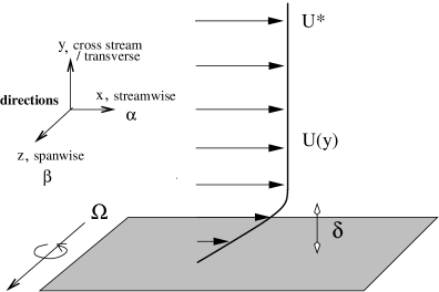
Figure 1: Yecko, Phys. Fluids

Let us now consider a frame rotating along the $z$-direction with a constant angular velocity $\Omega$ (see Fig.1). By applying the usual boundary layer scalings SchGer to the rotating Navier-Stokes equations, the nondimensional equations read in the limit of large ${\rm Re}$,

$${\partial u\over\partial x}+{\partial v\over\partial y}=0$$ (5)

$$u{\partial u\over\partial x}+v{\partial u\over\partial y}=-{\partial p\over\partial x}+{\partial^{2}u\over\partial y^{2}}+{1\over{\rm Re}{\rm Ro}}v$$ (6)

$$0=-{\partial p\over\partial y}-{1\over{\rm Ro}}u$$ (7)

where the Rossby number is defined such as ${\rm Ro}=U^{*}/2\Omega\delta$ where $\delta$ stands for the displacement thickness ($\delta=\delta_{B}$ or $\delta_{S}$). Unless rotation is very strong (i.e. the rotation number ${\rm Rot}=(2{\rm Ro})^{-1}>>1$), the term ${1\over{\rm Re}{\rm Ro}}v$ is weak relative to the leading order terms (the strongest rotation numbers used in this study are ${\cal O}(1)$) and can thus be neglected in the streamwise momentum equation, (6). A non-rotating boundary layer profile such as the Blasius profile or AS profile, is then preserved in the presence of rotation PotCha although rotation calls for an added cross-stream base pressure gradient, $dP/dy=-{1\over{\rm Ro}}U(y)$ to balance the Coriolis force resulting from the streamwise velocity $U(y)$. The rotating asymptotic suction (RAS) profile continues to be an exact solution of the rotating Navier-Stokes equations if, in addition to the normal base pressure gradient, $dP/dy=-{1\over{\rm Ro}}U(y)$, a streamwise pressure gradient $dP/dx={1\over{\rm Re}{\rm Ro}}V$ is included in the base flow to balance the Coriolis term in the streamwise momentum equation.

In the following stability and transient growth calculations, the downstream variation of boundary layers is not accounted for. Two major hypothesis follow: (a) the streamwise profile is considered at a given streamwise position $x=x_{0}$, and (b) the transverse velocity component is discarded, i.e. we set $V=0$. For all RB computations and most RAS calculations (unless otherwise stated), the approximated profile ${(U(y),0,0)}$ will be hence used. However, as mentioned above, RAS flow with $V\neq 0$ is an exact parallel solution of the Navier-Stokes equations; it can thus be used as a test for the validity of the second hypothesis. In the Appendix, a comparison between the two possibilities $V\neq 0$ and $V=0$ is presented for RAS, based on growth rates and neutral curves of normal modes as well as transient growth. This study shows that the effect of the transverse velocity on the normal modes and transient properties is negligible.

III Mathematical Formulation

III.1 Linearized disturbance equations

In a frame rotating along the $z$-direction with a constant angular velocity $\Omega$ (see Fig.1), the dimensionless Navier-Stokes Equations read

$${\partial{\bf u}_{tot}\over\partial t}+{\bf u}_{tot}\cdot\nabla{\bf u}_{tot}+{1\over{\rm Ro}}{\hat{z}}\times{\bf u}_{tot}=-\nabla p_{tot}+{1\over{\rm Re}}\nabla^{2}{\bf u}_{tot};~{}~{}~{}\nabla\cdot{\bf u}_{tot}=0\$$ (8)

where non-dimensionalization has been performed using free stream velocity $U^{*}$, displacement thickness $\delta$ ($=\delta_{B}$ or $\delta_{S}$), and pressure scale $\rho(U^{*})^{2}$. Two dimensionless number then arise: the Reynolds number ${\rm Re}=U^{*}\delta/\nu$ , and the Rossby number ${\rm Ro}=U^{*}/2\Omega\delta$.

Following standard methods, the base state velocity footnote $(U(y),V,0)$ and pressure $P(y)$ are perturbed by adding an infinitesimal disturbance $(u_{p},v_{p},w_{p})$ and $p_{p}$. These linear perturbations can be assumed to satisfy a modal behavior in $x$,$z$, viz.

$$(u_{p},v_{p},w_{p};p_{p})=({u}(y,t),{v}(y,t),{w}(y,t);{p}(y,t))e^{i(\alpha x+\beta z)}\;,$$ (9)

where $\alpha,\beta$ are assumed to be purely real. By using normal velocity ${v}(y,t)$ and normal vorticity

$${\zeta}(y,t)=i\beta{u}-i\alpha{w},$$ (10)

the linear dynamics is described by one equation governing normal velocity ${v}$:

$$(\frac{\partial}{\partial t}+i\alpha U+VD)(D^{2}-k^{2}){v}-i\alpha(D^{2}U){v}+{1\over{\rm Ro}}i\beta{\zeta}-{1\over{\rm Re}}(D^{2}-k^{2})^{2}{v}=0,$$ (11)

and a second equation governing normal vorticity ${\zeta}$:

$$(\frac{\partial}{\partial t}+i\alpha U+VD){\zeta}-{1\over{\rm Ro}}i\beta{v}+i\beta(DU){v}-{1\over{\rm Re}}(D^{2}-k^{2}){\zeta}=0,$$ (12)

where $k^{2}\equiv\alpha^{2}+\beta^{2}$, $D\equiv d/dy$. Equation (11) (resp. (12)) is nothing but the Orr-Sommerfeld (resp. Squire) equation modified to account for rotation. Boundary conditions

$${v}=D{v}={\zeta}=0\;\;\;\;$$ (13)

should be imposed at the wall $(y=0)$ and in the far field $(y\rightarrow\infty)$. A dynamical system is thus defined for ${\bf{q}(y,t)}=({v}(y,t),{\zeta}(y,t))^{T}$.

III.2 Normal mode approach

In this work, we study the above problem using two different approaches: the normal mode approach (cf asymptotic dynamics) and the non-normal approach (cf transient dynamics). The first approach consists in recasting the problem in §III(A) into an eigenvalue problem by assuming ${\bf q}={\bf{\tilde{q}}(y)}e^{-i\omega t}$ where ${\bf{\tilde{q}}}=({\tilde{v}},{\tilde{\zeta}})^{T}$ and $\omega=\omega_{r}+i\omega_{i}$ are complex. Clearly a mode having $\omega_{i}>0$ is unstable. Equations (11)-(12) can then be written

$$i\omega{\bf M{\tilde{q}}}={\bf L{\tilde{q}}}$$ (14)

where

$${\bf M}=\begin{pmatrix}D^{2}-k^{2}&0\\ 0&1\end{pmatrix}\;\;,\;\;{\bf L}=\begin{pmatrix}{\cal L}_{OS}&{\cal R}_{OS}\\ {\cal R}_{SQ}&{\cal L}_{SQ}\end{pmatrix}$$ (15)

with

$${\cal L}_{OS}=(i\alpha U+VD)(D^{2}-k^{2})-i\alpha(D^{2}U)-{1\over{\rm Re}}(D^{2}-k^{2})^{2},$$ (16)

$${\cal L}_{SQ}=i\alpha U+VD-{1\over{\rm Re}}(D^{2}-k^{2}),$$ (17)

$${\cal R}_{OS}={1\over{\rm Ro}}i\beta,~{}~{}{\cal R}_{SQ}=i\beta(DU)-{1\over{\rm Ro}}i\beta$$ (18)

It should be emphasized that as a result of rotation, the Orr-Sommerfeld equation is explicitly coupled to the Squire equation since both ${\cal R}_{OS}$ and ${\cal R}_{SQ}$ are nonzero while only the Squire equation is coupled through ${\cal R}_{SQ}$ in the absence of rotation. These equations together with the boundary conditions

$${\tilde{v}}=D{\tilde{v}}={\tilde{\zeta}}=0\;\;\;\;$$ (19)

imposed at the wall $(y=0)$ and in the far field $(y\rightarrow\infty)$ define the eigenvalue problem to be solved. A Chebyshev collocation algorithm developed in previous work YZF is implemented. First the semi-infinite domain is approximated by a sufficiently large interval $[0,L]$, a method known to be effective ButFar . In practice, the domain extended to sixteen displacement thicknesses $\delta$, $L=16~{}\delta$. This spatial interval is then mapped to the interval $[-1,1]$. Finally eigenfunctions are expanded into Chebyshev polynomials. The number $N$ of polynomials was generally $N=75$, although as many as $N=125$ were used to give improved accuracy in some calculations. Collocation points are the standard Gauss-Lobatto points. The eigenvalue problem (14) and boundary conditions (19) are then transformed into a corresponding $2N\times 2N$ matrix problem. To facilitate calculation, the eigenvalue problem (14) is actually written as

$$i\omega{\bf{\tilde{q}}}={\bf{\cal L}{\tilde{q}}}~{}~{}\hbox{with }~{}~{}{\bf{\cal L}}\equiv{\bf M}^{-1}{\bf L}\;.$$ (20)

III.3 Transient Growth Calculations

Transient amplification calculations have also been implemented on the problem in §III(A) according to the singular value decomposition (SVD) method given by Reddy and Henningson RedHen and the algorithms published in Ref. SchHen, . The main steps of the method are briefly described below; more details can be found in the references. First, the standard kinetic energy norm

$$||{\bf q(t)}||^{2}_{E}=\int_{0}^{L}(|Dv|^{2}+k^{2}|v|^{2}+|\zeta|^{2})dy$$ (21)

is used to measure the magnitude of a disturbance ${\bf q(t)}$ at time $t$. At time $t$, one can define

$$G(t)=\sup_{{\bf q}(0)\neq 0}~{}{||{\bf q(t)}||^{2}_{E}\over||{\bf q(0)}||^{2}_{E}}=||e^{i{\cal L}t}||^{2}_{E}\;,$$ (22)

where ${\bf q(0)}$ is an initial disturbance and ${\cal L}$ is the linear operator defined in (20). This quantity $G(t)$ represents the maximum possible energy amplification at time $t$, optimized over all possible initial disturbances. Finally the maximum or optimal growth is defined as $G_{MAX}=\sup_{t\geq 0}G(t)$. The peak value $G_{P}({\rm Ro},{\rm Re})\equiv\sup_{\alpha,\beta}G_{MAX}(\alpha,\beta,{\rm Ro},{\rm Re})$ can also be computed. Note that $G_{MAX}$ is associated with a particular initial disturbance which reaches $G_{MAX}$ at a specific time $t_{MAX}(\alpha,\beta,{\rm Ro},{\rm Re})$ such that $G_{MAX}=G(t_{MAX})$. Similarly one may define a specific time $t_{p}({\rm Ro},{\rm Re})$ related to $G_{P}$.

The quantity $G(t)$ is obtained as follows. Assume that the eigenvalues of (20)-(19) are sorted in order of decreasing imaginary part $\omega_{i}$. One can approximate $G(t)$ by computing the maximum possible energy amplification at time $t$, optimized over all possible initial combinations of the $K$ eigenfunctions associated with the first $K$ eigenvalues of (20). In this case, it is possible to transform the energy norm of the matrix exponential (22) to an ordinary 2-norm via the following equation

$$||e^{i{\cal L}t}||^{2}_{E}\approx||{\bf F}e^{-i\Lambda t}{\bf F^{-1}}||^{2}\;,$$ (23)

where $\Lambda$ is a $K\times K$ diagonal matrix with the first $K$ eigenvalues ${\omega_{1},\omega_{2},...,\omega_{K}}$ along the diagonal and ${\bf F}$ is obtained by Cholesky factorization of $K\times K$ Hermitian matrix ${\bf{\cal M}}={\bf F^{H}F}$ which is calculated using the inner product of the $K$ eigenfunctions of (20), the inner product used being the same as the one defining the norm (21).

The approximation of (23) is a result of the finite number $K$ used in the expansion. Following Ref RSH, , $K$ is chosen such that convergence is reached; in practice, $K\approx 60$ was found to be sufficient. The 2-norm on the RHS of (23) can now be evaluated using SVD. This procedure gives both $G_{MAX}$ and the $K$ expansion coefficients of the disturbance associated with $G_{MAX}$ RedHen ; ButFar . Note that, since eigenfunctions have been expressed as an expansion in Chebyshev polynomials, all calculations are ultimately performed in terms of the Chebyshev expansion coefficients. In particular, the energy norm (21) and the weight matrix ${\bf{\cal M}}$ are easily recast in terms of the expansion coefficients using the properties of Chebyshev polynomials and their derivatives (for details see Ref. RSH, ).

IV RESULTS

IV.1 Modal Stability Properties

It can be shown that within inviscid theory, Hart ; LezJon the stability of a rotating shear flow is analogous to that of Boussinesq convection in which the total base vorticity $(2\Omega-dU/dy)$ plays the role of temperature gradient. The dimensionless instability criterion then states that total vorticity must be negative somewhere in the flow Hart i.e.

$${\rm Ro}~{}{dU\over dy}>1\;.$$ (24)

The relative vorticity of the base flow $-dU/dy$ which is directed along the $z$ direction, is always negative for both RB and RAS flows. Positive Rossby ${\rm Ro}>0$, thus corresponds to oppositely directed rotation and flow vorticity, that is why it is referred to, in the geophysical literature, as anti-cyclonic. This is the region we will consider here since negative Rossby ${\rm Ro}<0$ correspond to cyclonic case where this instability disappears.

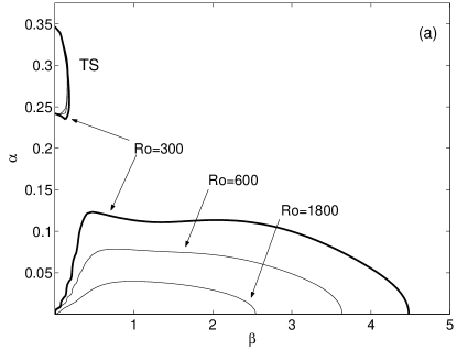
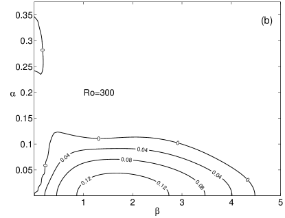
Figure 2: Yecko, Phys. Fluids

Neutral stability curves of RB flow at ${\rm Re}=600$ and several Rossby numbers are shown in Fig. 2a. The region identified as “TS” corresponds to the (rotationally modified) Tollmien-Schlichting modes of the non-rotating Blasius flow. The TS region is only slightly modified by rotation, becoming discernibly larger only when ${\rm Ro}$ is below $300$. The lower curves in Fig. 2a, identified by their ${\rm Ro}$ values, delineate the region of rotational instability. The largest growth rates are found for streamwise uniform modes ($\alpha=0$) having a non-zero spanwise wavenumber $\beta$ (Fig. 2b), that depends on the value of Ro, in agreement with previous results for other rotating shear flows. Hart ; LezJon ; AlfPer ; YFMR The extent of the rotationally unstable region grows rapidly with rotation, and is quite large at ${\rm Ro}=300$ which is the strongest rotation depicted in figure Fig. 2a. Ultimately, this instability is suppressed for very strong rotation as examined below. Note that the rotational instability takes on much larger growth rates than the TS instability, as illustrated by the curves of constant growth rate shown in Fig. 2b for the case ${\rm Re}=600$, ${\rm Ro}=300$. More precisely the largest TS growth rate is found in this case to be $\sup_{\alpha,\beta}(\omega_{i})_{TS}=0.006$ while the maximum value in Fig.2b is $\sup_{\alpha,\beta}\omega_{i}=0.145$

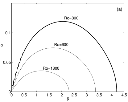
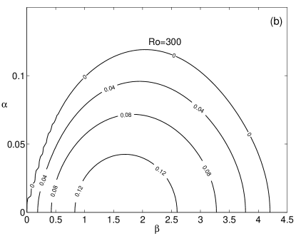
Figure 3: Yecko, Phys. Fluids

As in RB flow, an anti-cyclonic rotation for RAS leads, if not too strong, to a rotationally-induced instability which also reaches its maximum at $\alpha=0$, while a cyclonic rotation (${\rm Ro}<0$) is stabilizing. These rotationally unstable regions in $(\alpha,\beta)$-plane are presented in Fig. 3a for ${\rm Re}=600$ and several Rossby numbers ${\rm Ro}$. Note that growth rates of the rotational instability for RAS are of comparable magnitude to those found for RB flow (see Fig.3b for the case ${\rm Ro}=300$ where $\sup_{\alpha,\beta}\omega_{i}=0.144$ is found). On the contrary, no TS neutral curves appear for RAS (Fig. 3a) for ${\rm Re}=600$. Recall that the AS profile is known to be much more stable with respect to TS instability compared with non-rotating Blasius flow. This effect is very apparent in the large critical Reynolds number of the AS profile (${\rm Re_{c}}=54370$); DR RAS flow thus lacks TS instability at ${\rm Re}=600$.

Re-stabilization –

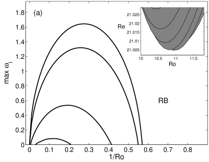
Figure 4: Yecko, Phys. Fluids

In RB flow, the condition for instability (24) corresponds to $1/{\rm Ro}<0.5714$foot57 while in RAS flow the condition becomes $1/{\rm Ro}<1$. The re-stabilization of rotating boundary layer flows by strong anti-cyclonic rotation is confirmed by numerical computations. The curves in Fig. 4 represent the largest growth rates ${\rm max}~{}\omega_{i}$ of this rotational instability found in the $(\alpha,\beta)$-plane as a function of $1/{\rm Ro}$ (this maximum was always found to occur for $\alpha=0$). At the largest Reynolds number depicted in Fig. 4a, ${\rm Re}=6000$, re-stabilization of RB flow occurs at $1/{\rm Ro}\approx 0.57$ while for RAS, re-stabilization occurs at $1/{\rm Ro}\approx 0.98$ when ${\rm Re}=60000$, in agreement with the predicted values. Large positive rotations have also been found to re-stabilize channel flows, LezJon ; MatAlf2001 at ${\rm Ro}$ values consistent with the vorticity criterion (24).

Since the rotational instability is fundamentally inviscid, the minimum Reynolds number below which the rotational instability is suppressed is quite low. The minimum Reynolds numbers below which no instability is found are ${\rm Re_{C}\approx 21}$ at ${\rm Ro_{C}\approx 10.9}$ for RB (see Fig. 4a) flow and ${\rm Re_{C}\approx 25.9}$ at ${\rm Ro_{C}\approx 23.5}$ for RAS flow (see Fig. 4b).

IV.2 Transient Amplification

The effect of rotation on transient growth for the RB and RAS flows is quantified through the analysis of amplification gain $G_{MAX}(\alpha,\beta,{\rm Ro},{\rm Re})$ as a function of streamwise wavenumber $\alpha$, spanwise wavenumber $\beta$, Reynolds number and Rossby number. Note that, in calculating $G_{MAX}$ and $G_{P}$ values, a fixed time interval $[0,T]$ is used during which the maximum growth is allowed to occur; the value of $T$ required to capture the maximum varies with ${\rm Re}$ and is adjusted accordingly in the calculations.

Non-rotating boundary layer flows are known to display the following transient growth features: (i) the most amplified disturbances tend to be three-dimensional with $\beta\neq 0$ and $\alpha=0$; (ii) the peak amplification for large Reynolds number is proportional to the square of the Reynolds number i.e.

$$G_{MAX}\propto\frac{{\beta}^{2}{\rm Re}^{2}T(k,\alpha{\rm Re})}{{k}^{2}}\;,$$ (25)

where it is recalled that $k^{2}=\alpha^{2}+\beta^{2}$ and $T$ is a function of $k$ and $\alpha{\rm Re}$ only; (iii) the time to achieve peak amplification increases linearly with the Reynolds number i.e. $t_{MAX}\propto{\rm Re}$. For rotating boundary layers, scaling (25) or its straightforward consequence $G_{P}\propto{\rm Re}^{2}$ is not preserved as shown below.

For non-rotating boundary layers $(U(y),0,0)$, the Reynolds scalings rely on the following statements (see also Ref.SchHen, ): upon performing the rescalings ${\hat{t}}=t/{\rm Re}$, ${\hat{\zeta}}=\zeta/(\beta{\rm Re})$, ${\hat{v}}=v$, equations (11)-(12) become dependent only on $k^{2}$ and $\alpha{\rm Re}$ and the energy turns into

$$||{\bf q({\hat{t}})}||^{2}_{E}=\int_{0}^{L}(|D{\hat{v}}|^{2}+k^{2}|{\hat{v}}|^{2})dy+(\beta{\rm Re})^{2}\int_{0}^{L}(|{\hat{\zeta}}|^{2})dy\;.$$ (26)

When the Rossby number is present, the energy expression is still valid but, in addition to $k^{2}=\alpha^{2}+\beta^{2}$ and $\alpha{\rm Re}$, the parameters ${\rm Ro}$ and ${(\beta{\rm Re})^{2}\over{\rm Ro}}$ explicitly appear in equations (11)-(12)

$$(\frac{\partial}{\partial{\hat{t}}}+i\alpha{\rm Re}U)(D^{2}-k^{2}){{\hat{v}}}-i\alpha{\rm Re}(D^{2}U){{\hat{v}}}+{1\over{\rm Ro}}i(\beta{\rm Re})^{2}{\hat{\zeta}}-(D^{2}-k^{2})^{2}{\hat{v}}=0,$$ (27)

$$(\frac{\partial}{\partial{\hat{t}}}+i\alpha{\rm Re}U){\hat{\zeta}}-{1\over{\rm Ro}}i{\hat{v}}+i(DU){\hat{v}}-(D^{2}-k^{2}){\hat{\zeta}}=0.$$ (28)

The standard arguments are thus no longer valid when the Rossby number is present, implying that the classical scalings will not be replicated. The numerical computations which confirm this idea, are presented below with the observed scalings.

Rotating Blasius boundary layer –

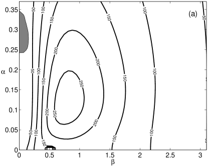
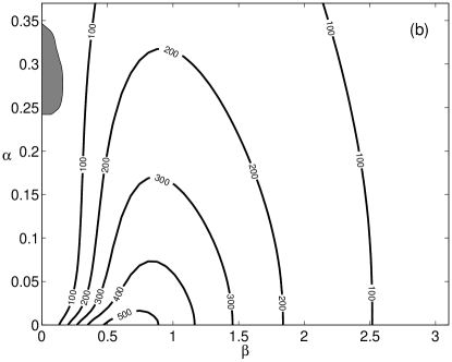
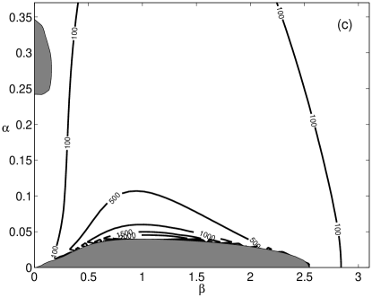
Figure 5: Yecko, Phys. Fluids

In Fig.5, level curves of $G_{MAX}$ in the $(\alpha,\beta)$-plane are presented for RB flow in three cases: weak cyclonic rotation ${\rm Ro}<0$ (Fig.5a), no rotation (Fig.5b), and weak anticyclonic rotation ${\rm Ro}>0$ (Fig.5c), the Reynolds number being always fixed at ${\rm Re}=600$ which is just above the critical value ${\rm Re}_{c}\approx 520$ for unstable Tollmien-Schlichting waves. The TS instability region is apparent along the $\alpha$-axis centered at $\alpha\approx 0.3$ and has only minor influence on the transient growth (see below).

In the absence of rotation, the peak $G_{MAX}$ value was found to occur at $\alpha=0$ and $\beta=0.651$ (Fig.5b), and to take the value $G_{P}=545.8$ ( $G_{P}=545.9$ with $N=75$ polynomials and $G_{P}=545.8$ with $N=125$). This value is in good agreement with other studies. ButFar ; BreKur ; CorBot From previous computations by Butler and FarrellButFar ($G_{P}=1514$ at ${\rm Re}=1000$) or Corbett and BottaroCorBot ($G_{P}=1515$ at ${\rm Re}=1000$) the scaling law $G_{P}=1.515\times 10^{-3}{\rm Re}^{2}$ should be the correct one for non-rotating Blasius flow. Using this latter formula, it is found that $G_{P}=545.4$ at ${\rm Re}=600$.

When the rotation is anti-cyclonic (Fig.5c) i.e. for ${\rm Ro}>0$, rotational instability of §IV(A) appears along the $\beta$-axis and the level curves of $G_{MAX}$ are distorted in the neighborhood of the highlighted region of unstable normal modes. Moreover, the $G_{MAX}$ values adjacent to the neutral curve are enhanced by the nearby modal instability, and the peak amplification occurs along the rotational neutral curve at $\beta\approx 1$. In such a case, transient growth must compete with the strong modal instability.

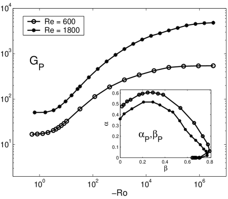
Figure 6: Yecko, Phys. Fluids

With cyclonic rotation (Fig.5a) i.e. for ${\rm Ro}<0$, $G_{MAX}$ values are reduced in magnitude everywhere in the $(\alpha,\beta)$-plane and the rotational instability is absent. In addition, $G_{P}$ is now found at non-zero streamwise wavenumber (for ${\rm Ro}=-1800$ and ${\rm Re}=600$, $\alpha\approx 0.12$), while the spanwise wavenumber slightly shifts from the value of the non-rotating case (for ${\rm Ro}=-1800$ and ${\rm Re}=600$, $\beta\approx 0.75$). An optimal disturbance (hereafter denoted by OD) with weak streamwise dependence ($\alpha\neq 0$) is often referred to as oblique, and is more typical of plane Couette flow than of boundary layer flow. Here, the obliquity is a consequence of the Coriolis effects. The ${\rm Ro}$ dependence of the peak growth $G_{P}$ is illustrated in Fig.6. Each point in this figure was obtained by first performing a calculation of $G_{MAX}$ throughout the $(\alpha,\beta)$-plane (like the one of Fig.5a), then finding the peak value, $G_{P}$, and the wavenumbers, $\alpha_{P}$ and $\beta_{P}$ at which the peak occurs. Two Reynolds numbers are shown: ${\rm Re}=600$, marked by open circles, and ${\rm Re}=1800$, marked by dots.

The inset of Fig.6 shows the location in the $\alpha-\beta$ wavenumber plane corresponding to the plotted $G_{P}$ values. When rotation is very weak, $G_{P}$ is found at $\alpha_{P}=0$, $\beta_{P}=0.651$; as rotation increases, the location of $G_{P}$ loops through the plane, eventually settling at $\beta_{P}=0$ for strong rotation, with a streamwise wavenumber $\alpha_{P}({\rm Re})$ dependent on the Reynolds number. The value $G_{P}=16.70$ is found at $\alpha_{P}=0.467$ for ${\rm Re}=600$ while $G_{P}=51.02$ is found at $\alpha_{P}=0.364$ when ${\rm Re}=1800$. These values are also recovered for strong values of anti-cyclonic rotation. The wavenumber $\alpha_{P}$ and $G_{P}$ values at strong rotation agree with two-dimensional non-rotating transient growth calculations. Butler & Farrell ButFar give $G_{P}=28$ at $\alpha_{P}=0.42$ for the best optimal 2D ($\beta_{P}=0$) disturbance for non-rotating Blasius flow at ${\rm Re}=1000$. At the same Reynolds number, we find $G_{P}=28.4$ for ${\rm Ro}=-0.5$ at $\alpha_{P}=0.42$. These findings are consistent with the idea that strong rotation imposes a two-dimensional Taylor-Proudman régime. LezJon ; Mutabazi

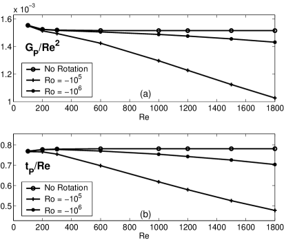
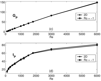
Figure 7: Yecko, Phys. Fluids

The ratio of the two $G_{P}$ curves in Fig.6 is a measure of the ${\rm Re}$ dependence of $G_{P}$ over a range of ${\rm Ro}$. From the figure, this dependence is clearly inconsistent with a $Re^{2}$ scaling throughout the entire ${\rm Ro}$ range. This ${\rm Re}$ dependence is explicitly shown in Fig.7a and 7c. For weak rotation (${\rm Ro}=-10^{6}$), $G_{P}/{\rm Re}^{2}$ possesses a weak ${\rm Re}$ dependence (Fig.7a) which strengthens for slightly stronger rotations (${\rm Ro}=-10^{5}$). In the strong rotation régime (Fig.7c), no simple ${\rm Re}$ dependence is found for $G_{P}$ in RB flow: although $G_{P}$ seems linear in ${\rm Re}$, a careful analysis reveals that this is not strictly correct. In addition, figure Fig.7c confirms that, for transient growth properties, the flow becomes increasingly two-dimensional in character as rotation increases. Note that, in a similar manner, the time $t_{p}$ is not linear in ${\rm Re}$ for weak rotation (${\rm Ro}=-10^{6}$) (Fig.7b) while we obtain scaling $t_{P}=0.78{\rm Re}$ with no rotation. In the strong rotation régime (Fig.7d), $t_{P}$ possesses no obvious scaling though one would guess by eye a $\sqrt{{\rm Re}}$ law, which is not confirmed by a rigorous fit.

Rotating asymptotic suction flow –

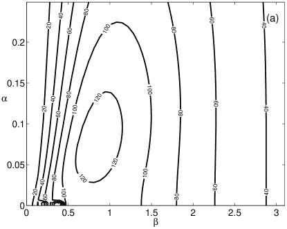
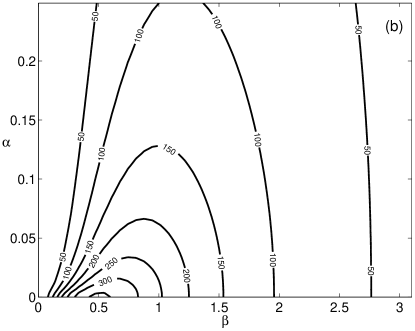
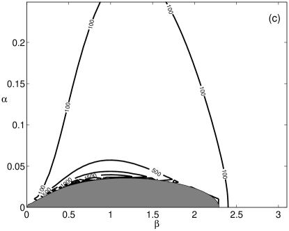
Figure 8: Yecko, Phys. Fluids

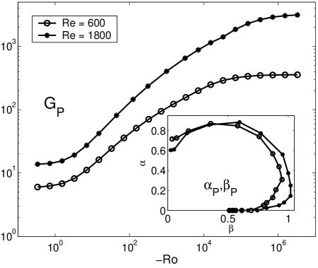
Figure 9: Yecko, Phys. Fluids

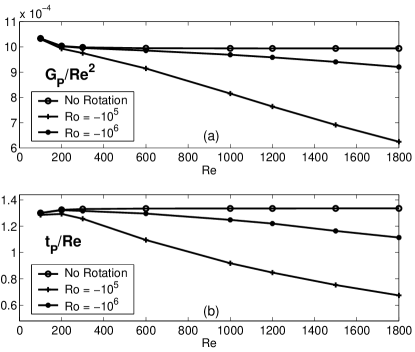
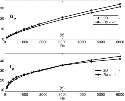
Figure 10: Yecko, Phys. Fluids

The qualitative features found for RB flow are also recovered for RAS flow; the following presentation can therefore be relatively terse. Figure 8 is the equivalent of Fig. 5, but for RAS flow at ${\rm Re}=600$. AS flow is well below its critical value $R_{c}=54370$ for TS instability, so no TS region is present. The most amplified disturbances in the absence of rotation (Fig.8b) are again streamwise uniform $(\alpha=0)$ while for weak cyclonic rotation (Fig.8a) they begin to show weak streamwise variability ($\alpha\approx 0.07$ for the case of Fig.8a). Figure 9 is the RAS flow equivalent of Fig. 6; here, again, both ${\rm Re}=600$, marked by open circles, and ${\rm Re}=1800$, marked by dots, are calculated. These are the only known calculations of transient growth in RAS flow. For AS flow (i.e. no-rotating case), the values of $G_{P}$ and $\beta_{P}$ have appeared in recent works: Ref. FranssonCorbett, provides a scaling law of the form $G_{P}=0.99Re^{2}$ which gives e.g. $G_{P}=356.4$ at $Re=600$. In the limit of very weak rotation, we find $G_{P}({\rm Re}=600)=358.12$ (or, when the transverse velocity $V$ is included, $G_{P}({\rm Re}=600)=356.74$, in good agreement with Ref.FranssonCorbett, ). As in RB, scalings $G_{P}\propto{\rm Re}^{2}$ and $t_{P}\propto{\rm Re}$ are not recovered, except for very weak rotation (Fig.10a and 10b). Again as in RB, a careful analysis does not reveal a clear scaling for $G_{P}$ and $t_{P}$ in the strong rotation régime (Fig.10c and 10d) though one would guess by eye a scaling in ${\rm Re}$ and $\sqrt{{\rm Re}}$ respectively.

The inset of Fig.9 shows the location in the $\alpha-\beta$ wavenumber plane corresponding to the plotted $G_{P}$ values. As in RB, the optimal disturbance in RAS flow makes an excursion in wavenumbers, starting at $\alpha_{P}=0$, $\beta_{P}=0.499$ ($\beta_{P}=0.530$ when $V$ is included) for very weak rotation, looping through the plane and settling on $\beta=0$ and a ${\rm Re}$-dependent $\alpha_{P}({\rm Re})$ when rotation is strong. For instance, the value $G_{P}=5.736$ is found at $\alpha_{P}=0.670$ for ${\rm Re}=600$ while $G_{P}=13.12$ is found at $\alpha_{P}=0.617$ for ${\rm Re}=1800$. When $V$ is included, these values shift to $G_{P}=5.661$ at $\alpha_{P}=0.675$ for ${\rm Re}=600$ and $G_{P}=13.01$ at $\alpha_{P}=0.621$ for ${\rm Re}=1800$. These same values are also recovered for strong values of anti-cyclonic rotation.

IV.3 Optimal Disturbances

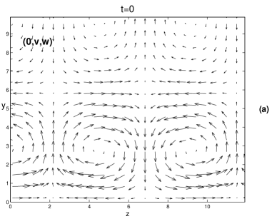
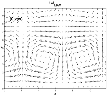
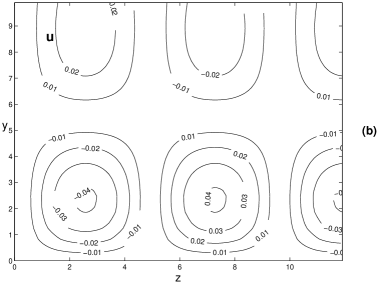
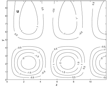
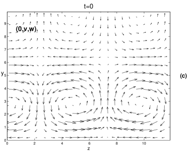
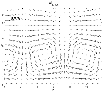
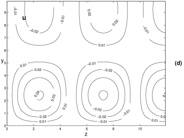
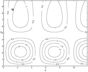
Figure 11: Yecko, Phys. Fluids

The most amplified disturbances in cyclonic RB and RAS flows possess a non-null streamwise wavenumber: they thus correspond to oblique vortices. The flow field of these disturbances can be calculated from its expansion coefficients, already obtained in the SVD solution of $G_{MAX}$. An example of the optimal disturbance (OD) in a weakly rotating RB flow, at ${\rm Re}=600$, ${\rm Ro}=-1\times 10^{6}$, is depicted in Fig.11 and can be compared to the OD for the classical Blasius flow at the same Reynolds. In figures Fig.11 and 12, the velocity field $v{\hat{y}}+w{\hat{z}}$ and the streamwise velocity component $u$ are shown at a given streamwise location ($x=0$). Due to the similarity of the optimal disturbances for RB and RAS flows, RAS examples are not shown.

While the OD in RB at very weak rotation ${\rm Ro}=-1\times 10^{8}$ is indistinguishable from the OD in non-rotating Blasius flow at both $t=0$ and $t=t_{P}$, this is not so for larger but still weak rotations. Indeed the OD in RB at ${\rm Ro}=-1\times 10^{6}$ (Fig.11 a) –which resembles with apparent counter-rotating streamwise rolls, the OD in non-rotating Blasius flow at $t=0$ (Fig.11c)– is such that the extrema of streamwise velocity $u$ (Fig.11b) are not precisely aligned with the up- and down-flows (Fig.11a) between the vortices, as found in non-rotating Blasius flow (Figs.11c,d). This offset is still found in the OD at its greatest amplification at $t=t_{P}$. Except for a shift of phase, little change is seen in the $u$ field. This explains why the $G_{P}$ value is not too different from the one found in the non-rotating limit. The kinetic energy of the OD is initially mainly in the $v$ or $w$ components and not in $u$ component. At $t=t_{P}$ it is contained mainly in $u$ field.

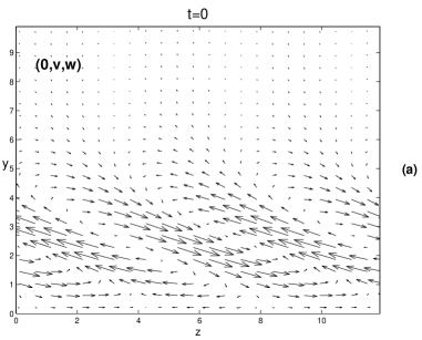
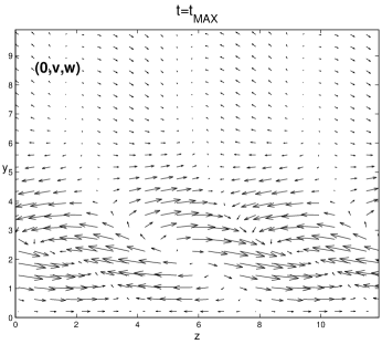
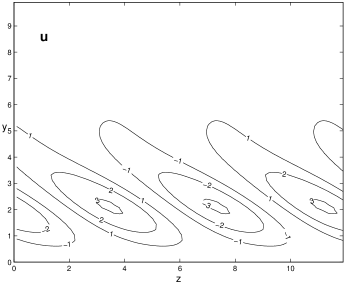
Figure 12: Yecko, Phys. Fluids

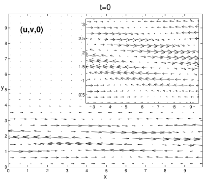
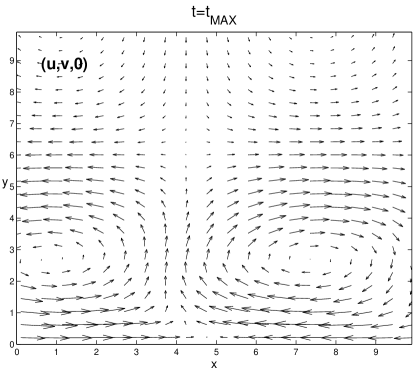
Figure 13: Yecko, Phys. Fluids

The above features are enhanced at stronger rotations as depicted in Fig.12, where ${\rm Ro}=-1800$: even the OD at $t=0$ being profoundly modified. Finally, at very strong rotation (e.g. ${\rm Ro}=-1$ in Fig.13), two-dimensionality is imposed in the $x-y$ plane and the OD at $t=0$ (Fig.13) clearly exhibits the characteristic tilting against the shear of the 2D Orr mechanism. At $t=t_{P}$, the shear has evolved the initial disturbance into vortices counter-rotating along the $z$-axis (Fig.13).

V Conclusions

This work has expanded on previous studies of boundary layer flows to account for frame rotation. In particular, the temporal evolution of three-dimensional disturbances has been studied for RB and RAS boundary layer flows in the presence of spanwise rotation. Normal mode and transient growth disturbances properties were calculated and compared for the two flows. Rotational modal instability, similar to that known for rotating channel and free shear flows, was found for weak anti-cyclonic rotation in RB and RAS; neutral curves, growth rates and the critical point were calculated for both flows. Rotating boundary layer flows were also found to exhibit transient growth. In the modally stable cyclonic regime the transient growth properties strongly depend on the rotation rate. In particular: (i) peak growth factors are reduced by rotation; (ii) even at weak rotation, the classical $Re^{2}$ dependence is not recovered; (iii) optimal disturbances take the form of oblique vortices which transform continuously from streamwise uniformity ($\alpha=0$) when rotation is very weak to spanwise uniformity ($\beta=0$) when rotation is strong, this last feature being a consequence of a Taylor-Proudman régime.

It is anticipated that the results presented here may be useful in dealing with geophysical and astrophysical flows, where rotation is important and curvature is often negligible. Most noteworthy is the example of Keplerian flow in an accretion disk, where no purely hydrodynamic inviscid linear eigenvalue instability has been identified. A study of transient growth in two-dimensional accretion disks IK has recently been performed and further inquiry is already under way. The problems analyzed in this work constitute an interesting element of disk flow studies.

Finally let us mention that the longitudinal roll instability in rotating shear flow exhibits weak downstream development AlfPer . Because the development is weak and because a great deal of closely related previous work Johnson ; PotCha ; YFMR ; LezJon ; Hart is based on temporal theory, this study adopted a temporal framework. However recent spatial analyses of ordinary boundary layer transient growth Luchini12 ; AndBerHen ; TumRes are shown to be more realistic with respect to observations. White In future investigation, this aspect should be envisaged to complement the present temporal theory.

APPENDIX: The transverse velocity in the presence of rotation.

Transverse velocity $V$ is normally neglected in the classical temporal stability analysis of Blasius flow, being of the same order as other neglected terms. The effect of this assumption on the instability normal modes is well documented for non-rotating AS and Blasius flows (see standard references, e.g. Ref. DR, ). In this appendix, we examine the effect of this assumption on two aspects which have not been previously studied: (a) the effect of $V$ on transient growth properties with or without rotation; (b) the effect of $V$ on the rotational normal mode instability properties. We consider these two effects on the AS and RAS flows since they are true Navier-Stokes solution when $V$ is present which authorizes a quantitative comparison between the simplified analysis ($V=0$) and the complete one.

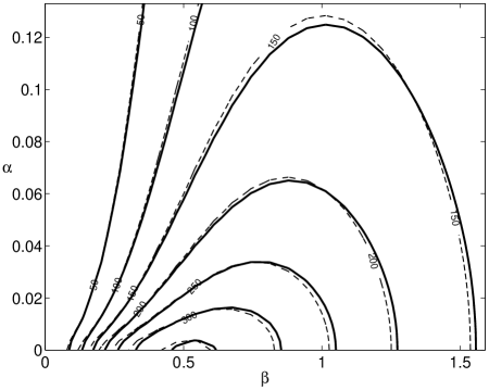
Figure 14: Yecko, Phys. Fluids

An overview of the effect of $V$ on the transient growth properties of the AS flow (i.e. non-rotating) can be found in Table I. Briefly, the neglect of $V$ has little effect on the peak growth factors $G_{P}$ of AS flow, less than one percent. The wavenumber of peak growth, $\beta_{P}$, is shifted to larger values when $V$ is included in AS calculations, but the shift is relatively small. The two cases are illustrated in Fig. 14 where level surfaces of $G_{P}(\alpha,\beta)$ are shown for the AS calculated with and without the $V$ term. As regard $t_{P}$ values, we obtain $t_{P}=1.145{\rm Re}$ when V is included which agrees with Ref.FranssonCorbett, and we find $t_{P}=1.331{\rm Re}$ when V is neglected.

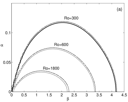
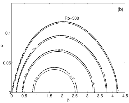
Figure 15: Yecko, Phys. Fluids

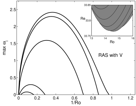
Figure 16: Yecko, Phys. Fluids

The effect of $V$ on the rotational instability neutral curves and growth rates is small, except near the critical point $({\rm Re}_{C},{\rm Ro}_{C})$. These properties are illustrated for RAS in Fig.15a, showing the shifted neutral curves, and Fig.15b, showing the modified growth rates. When $V$ is included, the location of the critical point shifts from ${\rm Re}_{C}=25.9,{\rm Ro}_{C}=23.5$ to ${\rm Re}_{C}=33.7,{\rm Ro}_{C}=14.6$, as seen in Fig.16 (compare to Fig.4(b)).

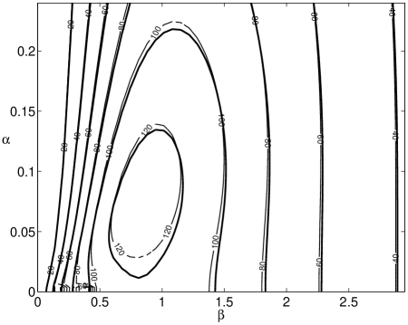
Figure 17: Yecko, Phys. Fluids

Under rotation, the effect of $V$ on the transient growth properties of the RAS remains negligible. To show this we display in Fig.17 the differences in peak growth factors $G_{P}$ calculated with and without the $V$ term for ${\rm Re}=600,{\rm Ro}=1800$.

Table 1: Peak transient growth quantities for non-rotating AS flows computed with and without the transverse velocity, $V$ term. Values for non-rotating Blasius flow with $V=0$ are given for the sake of completeness.

	Blasius	Blasius	AS	AS
	$Re=600$	$Re=1800$	$Re=600$	$Re=1800$
$G_{P}(V=0)$	545.93	4910.5	358.12	3220.2
$G_{P}(V\neq 0)$	—	—	356.74	3207.5
$\beta_{P}$(V=0)	0.651	0.651	0.499	0.499
$\beta_{P}(V\neq 0)$	—	—	0.529	0.530

Table I, Yecko, Phys. Fluids

List of Figure Captions

FIG. 1: Sketch of the flow configuration.

FIG. 2: (a) Neutral curves of RB flow at Reynolds number ${\rm Re}=600$ and various Rossby numbers ${\rm Ro}$; $\alpha$ and $\beta$ are the streamwise and spanwise wavenumber, respectively. (b) Curves of constant growth rate $\omega_{i}$ for RB flow at ${\rm Re}=600$ and ${\rm Ro}=300$.

FIG. 3: (a) Neutral curves of RAS flow at Reynolds number ${\rm Re}=600$ and various $Ro$; (b) Curves of constant growth rate $\omega_{i}$ for RAS flow at ${\rm Re}=600$ and ${\rm Ro}=300$.

FIG. 4: (a) Largest growth rates ${\rm max}~{}\omega_{i}$ for anti-cyclonic RB flow at Reynolds numbers $Re=25,60,600,6000$ (curves bottom to top); Inset: projection of the neutral surface $\omega_{i}(\beta,Re,Ro)=0$ onto the $Re-Ro$ plane, showing the critical point $Re_{C}=21.005,Ro_{C}=10.9$; (b) Same as (a) but for RAS at $Re=40,60,600,6000,60000$ (curves bottom to top); Inset: critical point $Re_{C}=25.9,Ro_{C}=23.5$.

FIG. 5: Level curves of $G_{MAX}$ in the $(\alpha,\beta)$-plane for RB flow at ${\rm Re}=600$ and for weak cyclonic $({\rm Ro}=-1800)$ rotation (a), no rotation (b), and weak anti-cyclonic $({\rm Ro}=1800)$ rotation (c). Regions of modal instability are shaded.

FIG. 6: Peak amplification factors $G_{P}$ of RB flow at ${\rm Re}=600$ and ${\rm Re}=1800$ as a function of cyclonic ${\rm Ro}<0$; Inset: corresponding location in the wavenumber $\alpha-\beta$ plane of the optimal disturbance associated with $G_{P}$ values in the figure; weak rotation cases lie along the $\beta$ axis while strong rotation cases lie along $\alpha$.

FIG. 7: (a) $G_{P}/{\rm Re}^{2}$ of RB flow as a function of ${\rm Re}$ for two weak rotation cases ${\rm Ro}=-10^{5}$, ${\rm Ro}=-10^{6}$ and no-rotation; (b) $t_{P}/Re$ of RB flow as a function of ${\rm Re}$ for the same cases as (a); (c) $G_{P}$ of RB flow as a function of ${\rm Re}$ for strong rotation, ${\rm Ro}=-1$, and two-dimensional disturbances; (d) $t_{P}$ of RB flow as a function of ${\rm Re}$ for the same cases as (c).

FIG. 8: Level curves of $G_{MAX}$ in the $(\alpha,\beta)$-plane for RAS flow at ${\rm Re}=600$ for weak cyclonic $({\rm Ro}=-1800)$ rotation (a), no rotation (b), and weak anti-cyclonic $({\rm Ro}=1800)$ rotation (c). Regions of modal instability are shaded.

FIG. 9: Peak amplification factors $G_{P}$ of RAS flow at ${\rm Re}=600$ and ${\rm Re}=1800$ as a function of cyclonic ${\rm Ro}<0$; Inset: corresponding location in the $\alpha-\beta$ plane of the optimal disturbance associated with $G_{P}$ values in the figure; weak rotation cases lie along the $\beta$ axis while strong rotation cases lie along the $\alpha$ axis.

FIG. 10: (a) $G_{P}/{\rm Re}^{2}$ of RAS flow as a function of ${\rm Re}$ for two weak rotation cases ${\rm Ro}=-10^{5}$, ${\rm Ro}=-10^{6}$ and no-rotation; (b) $t_{P}/Re$ of RAS flow as a function of ${\rm Re}$ for the same cases as (a); (c) $G_{P}$ of RAS flow as a function of ${\rm Re}$ for strong rotation, ${\rm Ro}=-1$, and two-dimensional disturbances; (d) $t_{P}$ of RAS flow as a function of ${\rm Re}$ for the same cases as (c).

FIG. 11: (a) Velocity vectors $v{\hat{y}}+w{\hat{z}}$ of the most amplified disturbance in cyclonic RB flow at ${\rm Re}=600$ and ${\rm Ro}=-10^{6}$. The disturbance is shown at $t=0$ (left) and at the time of maximum growth (right). (b) Streamwise velocity $u$ for OD of (a). (c) Velocity vectors $v{\hat{y}}+w{\hat{z}}$ for non-rotating Blasius flow at ${\rm Re}=600$. The disturbance is shown at $t=0$ (left) and at the time of maximum growth (right). (d) Streamwise velocity $u$ for OD of (c).

FIG. 12: (a) Velocity vectors $v{\hat{y}}+w{\hat{z}}$ of the most amplified disturbance in cyclonic RB flow at ${\rm Re}=600$ and ${\rm Ro}=-1800$. The disturbance is shown at $t=0$ (left) and at the time of maximum growth (right). (b)Streamwise velocity $u$ for OD of (a).

FIG. 13: Velocity vectors $u{\hat{x}}+v{\hat{y}}$ in the $x-y$ plane of the most amplified disturbance in cyclonic RB flow at ${\rm Re}=600$ and ${\rm Ro}=-1$. The disturbance is shown at $t=0$ (left) and at the time of maximum growth (right).

FIG. 14: Comparison of the level curves of $G_{MAX}$ in the $(\alpha,\beta)$-plane for AS flow calculated with $V$ included (solid curves) and $V$ neglected (dashed). The peak growth is found at $\alpha_{P}=0$ and $\beta_{P}=0.529$ (V included) or $\beta_{P}=0.499$ (V neglected).

FIG. 15: (a) Neutral curves of RAS flow at Reynolds number ${\rm Re}=600$ and three $Ro$; (b) Curves of constant growth rate $\omega_{i}$ for RAS flow at ${\rm Re}=600$ and ${\rm Ro}=300$. In the figure, the dashed curves correspond to calculations in which $V$ was neglected, reproducing Fig.3; the solid curves were computed with $V$ included.

FIG. 16: Largest growth rates ${\rm max}~{}\omega_{i}$ for anti-cyclonic RAS flow with $V$ included at Reynolds numbers $Re=40,60,600,6000,60000$ (curves, bottom to top); Inset: projection of the neutral surface $\omega_{i}(\beta,Re,Ro)=0$ onto the $Re-Ro$ plane, showing the critical point at ${\rm Re}=33.77$, ${\rm Ro}=14.5$. To be compared to Fig.4(b).

FIG. 17: Comparison of maximum transient growth level curves for RAS flow at ${\rm Re}=600,{\rm Ro}=1800$, calculated with $V$ included (solid curves) and $V$ neglected (dashed curves). The peak growth factor is $G_{P}=130.79$ ($V$ included) or $G_{P}=129.86$ ($V$ neglected).

References

- (1) P.G. Drazin and W.H. Reid Hydrodynamic stability (Cambridge Univ. Press, Cambridge, 1981).
- (2) A. Zebib and A. Bottaro “Goertler vortices with system rotation: Linear theory,” Phys. Fluids A 5(5) 1206 (1993).
- (3) A.H. Lefebvre Atomization and Sprays (Taylor & Francis, New York, 1989).
- (4) E.A. Spiegel and J.P. Zahn “The solar tachocline,” Astron. and Astroph. 265(1), 106 (1992).
- (5) J. Frank, A. King and D. Raine Accretion Power in Astrophysics (Cambridge University Press, Cambridge, 1992).
- (6) D.J. Tritton and P.A. Davies “Instabilities in geophysical fluid dynamics,” in Hydrodynamic Instabilities and the Transition to Turbulence, edited by H.L. Swinney and J.P. Gollub (Springer-Verlag, Berlin, 1985).
- (7) J.E. Hart “Instability and secondary motion in a rotating channel flow,” J. Fluid Mech. 45, 341 (1971).
- (8) D.K. Lezius and J.P. Johnston “Roll-cell instabilities in rotating laminar and turbulent channel flows,” J. Fluid Mech. 77, 153 (1975).
- (9) P.H. Alfredson and H. Persson “Instabilities in channel flow with system rotation,” J. Fluid Mech. 202, 543 (1989).
- (10) S. Yanase, C. Flores, O. Métais and J.J. Riley “Rotating free-shear flows: I. Linear stability analysis,” Phys. Fluids A5(11), 2725 (1993).
- (11) M.C. Potter and M.D. Chawla “Stability of boundary layer flow subject to rotation,” Phys. Fluids 14(11), 2278 (1971).
- (12) Lord Kelvin (W. Thompson) “Stability of fluid motion: rectilinear motion of viscous fluid between two parallel planes,” Phil. Mag. 24, 188 (1887).
- (13) W.M.F. Orr “The stability or the instability of the steady motions of a perfect liquid and of a viscous liquid,” Proc. R. Irish Acad. A 27, 9 (1907).
- (14) T. Ellingson and E. Palm “Stability of linear flow,” Phys. Fluids 18(4), 487 (1975).
- (15) M.T. Landahl “A note on an algebraic instability of inviscid parallel shear flows,” J. Fluid Mech. 98, 243 (1980).
- (16) L.S. Hultgren and L.H. Gustavsson “Algebraic growth of disturbances in a laminar boundary layer,” Phys. Fluids 24, 1000 (1981).
- (17) L. Boberg and U. Brosa “Onset of turbulence in a pipe,” Z. Naturforschung 43a, 697 (1988).
- (18) K.M. Butler and B.F. Farrell “Three-dimensional optimal perturbations in viscous shear flow,” Phys. Fluids A 4(8), 1637 (1992).
- (19) L.N. Trefethen, A.E. Trefethen, S.C. Reddy and T.A. Driscoll “Hydrodynamic instability without eigenvalues,” Science 261, 578 (1993).
- (20) S.C. Reddy and D.S. Henningson “Energy growth in viscous channel flows,” J. Fluid Mech. 252, 209 (1993).
- (21) S. Grossmann “The onset of shear flow turbulence,” Rev. Mod. Phys. 72(2), 603 (2000).
- (22) E. Reshotko “Transient growth: A factor in bypass transition,” Phys. Fluids 13(5), 1067 (2001).
- (23) P.J. Schmid and D.S. Henningson Shear Flow Instability (Springer-Verlag, New York, 2000)
- (24) M. Matsubara and P.H. Alfredsson “Disturbance growth in boundary layers subjected to free-stream turbulence,” J. Fluid Mech. 430, 149 (2001).
- (25) H. Schlichting and K. Gersten Boundary Layer Theory, 8th edition, Springer, Berlin (2000).
- (26) The Mathworks, Inc. MatLab 6.5 (R13) (2002).
- (27) T.H. Hughes and W.H. Reid “On stability of asymptotic suction boundary-layer profile,” J.Fluid Mech. 23, 715 (1965).
- (28) L.M. Hocking “Non-linear instability of the asymptotic suction velocity profile,” Q.J. Mech. Appl. Math. 28(3), 341 (1975).
- (29) A constant transverse base velocity is included in this discussion to include the RAS flow with . In the other cases, it will be turned off i.e. .
- (30) P. Yecko, S. Zaleski and J.-M. Fullana “Viscous modes in two-phase mixing layers,” Phys. Fluids 14(12), 4115 (2002).
- (31) S.C. Reddy, P.J. Schmid and D.S. Henningson “Pseudospectra of the Orr-Sommerfeld operator,” SIAM J. Appl. Math. 53(1), 15 (1993).
- (32) In Blasius flow the vorticity at the wall: .
- (33) K.S. Breuer and T. Kuraishi “Transient growth in two- and three-dimensional boundary layers,” Phys. Fluids 6(6), 1983 (1984).
- (34) P. Corbett and A. Bottaro “Optimal perturbations for boundary layers subject to stream-wise pressure gradient,” Phys. Fluids 12(1), 120 (2000).
- (35) I. Mutabazi, C. Normand and J.E. Wesfried “Gap size effects on centrifugally and rotationally driven instabilities,” Phys. Fluids A 4(6) 1199 (1992).
- (36) J.H.M. Fransson and P. Corbett “Optimal linear growth in the asymptotic suction boundary layer,” Eur.J. Mech. B. 22, 259 (2003).
- (37) P.J. Ioannou and A. Kakouris “Stochastic dynamics of Keplerian accretion disks,” Ap.J. 550, 931 (2001).
- (38) J.A. Johnson “The stability of shearing motion in a rotating fluid,” J. Fluid Mech. 17, 337 (1963).
- (39) P. Luchini “Reynolds-number-independent instability of the boundary layer over a flat surface,” J. Fluid Mech. 327, 101 (1996). and P. Luchini “Reynolds-number-independent instability of the boundary layer over a flat surface: optimal perturbations,” J. Fluid Mech. 404, 289 (2000).
- (40) P. Andersson, M. Berggren and D.S. Henningson “Optimal disturbances and bypass transition in boundary layers,” Phys. Fluids 11(1), 134 (1999).
- (41) A. Tumin and E. Reshotko “Spatial theory of optimal disturbances in boundary layers,” Phys. Fluids 13(7), 2097 (2001).
- (42) E.B. White “Transient growth of stationary disturbances in a flat plate boundary layer,” Phys. Fluids 14(12), 4429 (2002).