SLAC-PUB-9616 February, 2003 physics/0302044

Abstract Applets:
a Method for Integrating Numerical Problem-Solving
into the Undergraduate Physics Curriculum

Michael E. Peskin

Stanford Linear Accelerator Center
Stanford University, Stanford, California 94309 USA

ABSTRACT

In upper-division undergraduate physics courses, it is desirable to give numerical problem-solving exercises integrated naturally into weekly problem sets. I explain a method for doing this that makes use of the built-in class structure of the Java programming language. I also supply a Java class library that can assist instructors in writing programs of this type.

Submitted to Computing in Science and Engineering

1 Introduction

A typical upper-division undergraduate physics course, for example, the course in classical electrodynamics at the level of Griffiths’ text [1], involves extensive analytic problem solving. Students learn to solve Laplace’s equation in rectangular coordinates, in cylindrical coordinates, with Bessel functions, with Legendre polynomials. The methods taught are important in their own right and as methods to illustrate central physical concepts. But it would be better if numerical problem-solving methods were discussed at a similar level. Students today typically have in their dorm rooms, and even carry in their backpacks, computers with the power of a typical university central mainframe of the 1970’s. It would be wonderful to put this power to work both to developing intuition and in explicit problem-solving.

The inclusion of numerical calculations in the physics curriculum is even more important because our students typically go to careers, either in research or in industrial settings, in which the basic task is modelling of physical systems. Analytic methods are useful for estimates, or for working out the dependence on parameters, but understanding a realistic system in detail typically requires a computer simulation. So we should make clear to our students right away that it is straightforward to put the equations that appear in their classes onto a computer and obtain sensible physical results.

This problem is currently addressed in the physics curriculum in two ways. First, specific physics problems are encoded in computer programs which students can run as black boxes, changing the parameters and seeing what consequences develop. The ‘scripted applets’ of the Davidson College group represent a very beautiful development along this line [2]. Such black-box programs are useful in introductory courses, but, for upper-division courses, they do not teach all of the skills one would like to develop. These programs are time-consuming to write, and it is often the philosophy that students should not touch the code. (The Davidson applets are designed so that not even professors modify the code.) But we would like students to write some code, and to understand how simple sets of instructions can iterate to the patterns that solve interesting equations of Nature. Often in undergraduate mechanics courses, instructors give students differential equations to be integrated by commercial packages such as Maple or Mathematica. Such projects have a similar black-box approach.

The other common approach is a computational physics course, on the model of the textbooks of Gould and Tobochnik [3] and Koonin [4]. Such courses are often constructed around major projects. Students spend a large part of a semester learning a learing a computer environment, then construct an elaborate code for one particular application. Such a course is important to give students experience with large-scale computer applications and to begin studying sophisticated numerical methods. But it would be good also to allow students to do simpler numerical problems that tie in directly to material being covered in their core courses.

Ideally, a weekly problem set in mechanics or electrodynamics should consist of several analytical and one numerical problem. The reason this is not done as a matter of course is the difficulty of having students master the purely computer programming aspects of the task.

In this article, I propose a way of solving this problem. The method is based on the structure of the programming language Java. Java is an object-oriented computer language which allows programs that have a hierarchial structure. Thus, one can assign to students the writing of a small piece of code, perhaps one subroutine that carries out a numerical computation. This code can then fit together with a larger program that implements a graphical user interface for visualizing the results of the program. The user interface code can be assembled by the instructor; students need not be bothered by its complexity. Finally, the instructor’s task in writing this larger program can be simplified if the various user interface elements are drawn from a pre-assembled ‘class library’.

At heart, this is the familiar strategy of asking students to write a subroutine which can be tied to a larger package of code. The use of Java assists this in two ways. First, it allows the instructor to neatly encapsulate the part of the code for which the student is responsible, hiding the details of the graphical elements and user interface. Second, it makes available to the instructor a programming library that makes it rather simple to write graphical elements that are interesting and pleasing.

This strategy could also be carried out in other programming languages that allow easy access to graphical user interface components, for example, Visual Basic. The CUPS project has created a range of pleasing simulations in Pascal [5], and these are extensible by working at the code level. Java has the advantage that the same code runs on UNIX, Windows, or Macintosh systems, so that students can put together their assignments on whatever operating system is most convenient for them. In addition, Java belongs to a family of computer languages, including C, C++, and Pascal, in which numerical computations have a common syntax. The part of the code that the student must write is almost indistinguishable among these four languages, so their is no need for students to have prior experience in Java.

An extensive set of software resources for creating educational simulations in Java is being put together by Christian, Gould, and Tobochnik [6] as a part of their work for the second edition of the textbook [3]. In contrast to that work, I provide here a minimal set of Java resources to provide exercises of the type I have described.

In this paper, I present this method of constructing problems with numerical solutions. In Section 2, I present a sample numerical exercise that I have given on a problem set. In Section 3, I give some further examples of such numerical exercises. All of these examples are based on a relatively simple class library of graphical elements that are specifically useful for programming exercises of this type. In Section 4, I describe the basic structure and format of this library. To illustrate its features, the master program for the first exercise is discussed in detail. Section 5 presents some conclusions. Appendix A gives the complete documentation for the class library. Appendix B gives a list of the example programs included in the software distribution.

The Java code for the class library and for the example programs discussed in this article can be found in a tar file at the web site at which the eprint of this paper is posted [7].

2 Laplace Applet

Textbook discussions of Laplace’s equation (e.g. [1]) note the fact that a solution $\phi(x)$ is the average of the solution at neighboring points, and that this fact can be the basis for a numerical solution of Laplace’s equation. In this section, I will present a homework problem that allows a student to implement this observation in a numerical program and see it work.

Look at the computer program shown in Fig. 1. It is not so difficult to make sense of this program. Its idea is to sweep through an array phi[i][j], updating successive values. The programs tests for the maximum change over the array and quits when this is sufficiently small. The algorithm for updating the array is not given. But one can explain in words that each array element can be, successively, set equal to the average of its neighbors, and that the equilibration of this process yields a solution of the Laplace equation.

To implement this algorithm, it is necessary to modify only one line of the code, replacing the assignment to newphi by

$$\verb!double newphi = !$$

$$\hskip 21.68121pt\verb!(0.25)*(phi[i+1][j]+phi[i][j+1]+phi[i-1][j]+phi[i][j-1]);!\ .$$ (1)

This statement has the same form in C, C++, Pascal, or Java. It should be at least recognizable by students whose only programming experience is in Basic or FORTRAN.

import java.awt.*;
import java.awt.event.*;
import java.applet.Applet;

public class Laplace extends LaplaceGUI{
  double criterion = 1.0e-2;

  void solve(){
    double maxdiff = 1.0;
    int iteration = 0;
    while ( maxdiff > criterion){
      for (int n = 1; n <= 20; n++){
        maxdiff = 0.0;
        for (int i = 1; i < Nx; i++){
          for (int j =1 ; j < Ny; j++){
              /* check whether (i,j) is a cathode or ground point */
            if (normal(i,j) == false) continue;
              /* update the phi array  */
            double oldphi = phi[i][j];
              /*  put something more sensible here  : */
            double newphi = 33.0;
            phi[i][j] = newphi;
Ψ    /*  compute the criterion for stopping */
            double delta = Math.abs(newphi-oldphi);
            if (delta > maxdiff) maxdiff = delta;
          }
        }
        iteration++;
      }
      refreshPicture();
      Legend.write("max. diff : "+maxdiff+ "      "+iteration);
      if (timetostop) break;
    }
  }

Figure 1: The program Laplace.java.

The statement class Laplace extends LaplaceGUI indicates that the simple program Laplace.java shown in Fig. 1 is intended to work with functions and data structures defined in a parent program LaplaceGUI.java. This program, its parent PhysicsApplet.java, and a small file Laplace.html are given the directory Laplace in the software distribution mentioned at the end of the Introduction. These files can be made available for download on the course Web page. Compiling these programs together, one obtains a working simulation toy. The method of linking the programs depends on the precise operating system, but under UNIX (or Mac OS X) it is as simple as putting the four files in the same directory and typing javac Laplace.java. The compiled program, or ‘applet’, is then run by viewing the file Laplace.html with a Web browser. The student would not be expected to modify, or even open, any of these files except for the original Laplace.java. This file contains all of the physics; the others simply supply the computer interface.

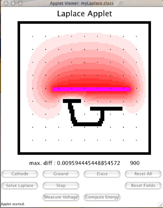
Figure 2: Working version of the Laplace applet.

The result of this process is a working application, a view of which is shown in Fig. 2. The applet shows a figure with a box that displays the values of the array phi in greyscale. In the specific example shown, phi is chosen to be a $100\times 100$ array. The box contain dots as fiducial marks at each tenth grid point, to facilitate specific numerical computations. By clicking on the buttons ‘Cathode’ and ‘Ground’, one can paint a set of boundary conditions with the mouse. Clicking on the button ‘Solve Laplace’ calls the method solve() in the program Laplace.java. As the array phi[i][j] is updated, the values of phi are displayed on the screen in grayscale. Clicking on the button ‘Measure Voltage’ and then clicking on the screen causes the value of phi at that point to appear as a label under the box.

Once the applet is programmed and working correctly, it can be used for many illuminating exercises. Some of these are qualitative problems, for example, illustrating the principle of a Faraday cage by placing small grounded conductors around a cathode. Others are quantitative, for example, working out the size of edge effects on the capacitance of a capacitor of finite size. To aid in the latter calculation, the button ‘Compute Energy’ computes the electrostatic energy stored in the configuration shown from a discrete approximation to the expression $\int d^{2}x\frac{1}{2}\epsilon_{0}E^{2}$. The problem set that contained this applet asked the student to implement a function Energy() that would be called by this button and return the result. The GUI would then take care of writing this result to the screen.

3 Further Examples

Many other computational exercises can be constructed along these lines. Eight additional applets are included with the software distribution. I describe two of these below.

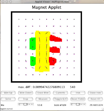
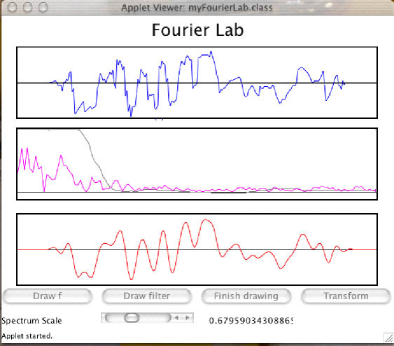
Figure 3: Working versions of the Magnet (left) and FourierLab (right) applets.

The left-hand side of Fig. 3 shows an applet that computs the magnetic fields in an array of wires and magnetic material that can be drawn on the screen. The situation is uniform in the third dimension, with current flowing up or down through the screen. A fixed current, up or down, is assigned to squares colored, respective, green or red. These squares can be painted with the mouse. The student can also color in regions to be filled with a linear magnetic material (‘iron’) with adjustible permeability $\mu$. The magnetic fields are generated from a vector potential $\vec{A}=(0,0,{\cal A})$, where ${\cal A}$ solves the Poisson equation

$$-\nabla^{2}{\cal A}=\mu{\cal J}\ ,$$ (2)

in which ${\cal J}$ is the current density in the wires (in A/m²). The equation can be solved by the same relaxation method discussed in the previous section for the Laplace equation. The problem set containing this applet explained the strategy, then asked the students to work out the details using their experience with the Laplace applet of Section 2. They were then asked to use this Magnet applet to to solve qualitative examples in the theory of magnetism and quantitative problems of magnet design.

The right-hand side of Fig. 3 shows an applet that can be used to illustrate the basic principles of signal analysis. The applet displays three boxes on the screen. In the upper box, a waveform can be entered, either from the computer program as a mathematical function or by drawing with the mouse. The center box shows the (modulus of the) Fourier transform of the waveform. This is multiplied by a filter function which, again, can either be supplied by the program or drawn on the screen. To present this applet on a problem set, I supplied to the students five files: FourierLab.java, FourierTransform.java, FourierLabGUI.java, PhysicsApplet.java, and FourierLab.html. The last of these is simply used to display the compiled program. The file FourierLab.java contains the functions defining the initial waveform and filter. The file FourierTransform.java contains the methods called by the button ‘Transform’. The remaining two Java programs define the graphical user interface and are not meant to be modified by the student. They do not contain any of the physics of the computation.

The contents of FourierTransform.java given to the student are shown in Fig. 4. The structure is based on notions of object-oriented programming, but it is self-explanatory. The real-space function is a real-valued function $f(x)$, represented as an array f[n], $n=0,\ldots,(N-1)$. The real and imaginary parts of the Fourier Transform are represented as arrays fcos[m] and fsin[m], $m=0,\ldots,N/2$. Using only the basic understanding of the treatment of arrays in any familiar programming language, it is straightforward to complete the Fourier transform algorithms so that they work correctly. (Java does have the peculiar feature that $\sin x$, $\cos x$ and $\pi$ are written Math.Sin(x), Math.Cos(x), and Math.PI; students must be told about this.) In principle, one could build different versions of FourierTransform.java from this basic structure, incoporating different algorithms for computing the Fourier Transform.

public class FourierTransform{

    int Nx, N2;
    double[] f, fcos, fsin;

    FourierTransform(int N){
        Nx = N;
        N2 = Nx/2;
        f = new double[Nx];
        fcos = new double[N2+1];
        fsin = new double[N2+1];
    }

    void Transform(){
        for (int i = 0; i <= N2 ; i++){
Ψ    double Tc = 0.0;
Ψ    double Ts = 0.0;
            for (int j = 0; j < Nx ; j++){
ΨΨ/*  do something intelligent here   */
            }
            fcos[i] = Tc;
            fsin[i] = Ts;
Ψ}
    }

    void InverseTransform(){
        for (int i = 0; i < Nx ; i++){
Ψ    double T = fcos[0] + fcos[N2];
            for (int j = 1; j < N2 ; j++){
ΨΨ/*  do something intelligent here   */
            }
            f[i] = 0.0;
Ψ}
    }
}

Figure 4: The class FourierTransform.java, as provided to the student.

4 Construction of the Laplace Applet

The computer programs described in the previous two sections are constructed from a simple program, containing the actual physics and accessible to the student, and a more complex user interface program whose contents the student can ignore. Up to now, I have not discussed any aspect of the Java programming language. However, the object-oriented nature of this language is the key to the way that these programs are structured. In this section, I will first review some notions of object-oriented programming and then explain how these ideas are applied in the specific case of the Laplace applet.

In object-oriented programming, the basic element of a program is a ‘class’, a set of data variables together with function (‘methods’) that act on these variables. One class can be created from another in a parent-daughter relation. The daughter class is said to ‘inherit’ the variables and methods of the parent; new variables and methods intrinsic to the daughter can be added to these. In this way, a complex structure can be built up in stages. It is possible to define an ‘abstract class’ in which one or more methods are defined in principle but are not implemented. An abstract class cannot be created (‘instantiated’) in a computer program. However, a daughter of the abstract class which defines the required methods can be created and used. In Java, each individual class A is defined in a separate file A.java.

The Java language defines an ‘applet’, a mini-program accessible through a Web browser, as a predefined parent class. This Applet class manages the window in which the program appears and provides methods to draw in this window.

The definition of the Laplace applet starts from a parent class PhysicsApplet which is a daughter class of Applet. This class defines various user interface elements that are useful in constructing problem set applets of the type that I have presented above. A complete documentation of the classes, variables, and methods of PhysicsApplet is given in Appendix A. PhysicsApplet is an abstract class that leaves a large number of methods undefined. The Java language contains many hooks to graphical elements, making it straightforward to construct basic user interfaces. There are many excellent books that describe user interface programming in Java [8, 9] However, I hope that the collection of specialized elements contained in PhysicsApplet will make it even a step easier for instructors to build their own programs of the type illustrated above.

The class LaplaceGUI is constructed as a daughter class of PhysicsApplet. The construction this class puts into the applet the specific displays and buttons described in Section 2. LaplaceGUI is still an abstract class. It defines almost all of the methods of PhysicsApplet but leaves undefined the methods solve(), which actually carries out the solution of Laplace’s equation, and Energy(), which computes the electrostatic energy. When the class Laplace adds a definition of solve() to this structure, as shown in Fig. 1, and also a definition of Energy(), all needed methods are defined and the class can be instantiated. In the writing of the Laplace class, the definitions of all of the other methods of LaplaceGUI can remain hidden.

The code for the class LaplaceGUI is shown in Figs 5–8. The program is lengthy, but it is all straightforward bookkeeping of the graphical elements.

The program begins by defining the basic array phi involved in the numerical computation, an array of integers State that keeps track of the boundary conditions drawn by the user, a graphic element of type ArrayDisplay, which produces the large square in described for the applet. and a graphic element of type TitleBanner, which displays a caption under this square.

The next segment of the program defines integer constants that label the options for the behavior of various elements of the program. Books on graphical user interfaces (notably [10]) ask that a user interface be ‘modeless’, so that the user has as many options as possible at any given time. The price of this feature is a complex programming style. My philosophy is just the reverse. I would like to make the programming task as easy as possible for the instructor, even if this costs the user some flexibility. Thus, the programming style is completely modal.

import java.awt.*;
import java.awt.event.*;
import java.applet.Applet;

abstract public class LaplaceGUI extends PhysicsApplet{

  double[][] phi;
  int[][] State;
  ArrayDisplay D;
  TitleBanner Legend;
  double CathodeV = 100.0;
     // mouse modes:
  static final int NormalMode = 0;
  static final int CathodeMode = 1;
  static final int GroundMode = 2;
  static final int EraseMode = 3;
  static final int MeasureMode = 4;
     // button codes:
  static final int FieldResetCode = 1;
  static final int AllResetCode = 2;
  static final int MeasureECode = 3;
  static final int StartCode = 4;
  static final int StopCode = 5;
    // array states:
  static final int NormalState = 0;
  static final int CathodeState = 1;
  static final int GroundState = 2;

  LaplaceGUI(){
    super("Laplace Applet",100,100,4,100);
    phi = new double[Nx+1][Ny+1];
    State = new int[Nx+1][Ny+1];
    for (int i = 0; i <= Nx; i++){
      for (int j = 0; j <= Ny; j++){
         phi[i][j] = 0.0;
         State[i][j] = 0;
       }
    }
  }

Figure 5: The class LaplaceGUI.java, part 1

  void resetArrays(){
      for (int mx = 0; mx <= Nx; mx++){
        for (int my = 0; my <= Ny; my++){
          if (State[mx][my] == 0)  phi[mx][my] = 0.0;
        }
      }
      refreshPicture();
    }

    void resetAll(){
      for (int mx = 0; mx <= Nx; mx++){
        for (int my = 0; my <= Ny; my++){
         phi[mx][my] = 0.0;
         State[mx][my] = 0;
        }
      }
      refreshPicture();
    }

  void buildPicture(){
    D = new ArrayDisplay(phi,State, Color.red,Color.black);
    Picture.add(D,"Center");
    Legend = new TitleBanner(" ", 16);
    Picture.add(Legend,"South");
  }

  void refreshPicture(){
    D.refresh();
  }

Figure 6: The class LaplaceGUI.java, part 2

  void buildControls(){
    Controls.setLayout(new GridLayout(0,4,10,10));
    ModeButton B1 = new ModeButton("Cathode", CathodeMode);
    Controls.add(B1);
    ModeButton B2 = new ModeButton("Ground", GroundMode);
    Controls.add(B2);
    ModeButton B3 = new ModeButton("Erase", EraseMode);
    Controls.add(B3);
    CommandButton B4 = new CommandButton("Reset All", AllResetCode);
    Controls.add(B4);
    CommandButton B5 = new CommandButton("Solve Laplace", StartCode);
    Controls.add(B5);
   CommandButton B6 = new CommandButton("Stop",StopCode);
    Controls.add(B6);
    Label B7 = new Label(" ");
    Controls.add(B7);
    CommandButton B8 =
                 new CommandButton("Reset Fields",FieldResetCode);
    Controls.add(B8);
    Label B9 = new Label(" ");
    Controls.add(B9);
    ModeButton B10 = new ModeButton("Measure Voltage", MeasureMode);
    Controls.add(B10);
    CommandButton B11 =
                 new CommandButton("Compute Energy", MeasureECode);
    Controls.add(B11);
    Label B12 = new Label(" ");
    Controls.add(B12);
  }

  Color findColor(double A, int S){
    if (S == CathodeState)  return D.Color2;
    if (S == GroundState)   return D.Color1;
    int colorm =  (int) ( 10.0 * A/CathodeV);
    return D.DisplayColors[colorm];
  }

  void writeFieldValue(double Val, int mode){
    if (mode == MeasureMode) Legend.write(" Voltage = " + Val);
  }

Figure 7: The class LaplaceGUI.java, part 3.

  void setArrays(int i, int j, int mode){
    if (mode == CathodeMode){
      phi[i][j] = CathodeV;
      State[i][j] = CathodeState;
    } else if (mode == GroundMode){
      phi[i][j] = 0.0;
      State[i][j] = GroundState;
    } else if (mode == EraseMode){
      phi[i][j] = 0.0;
      State[i][j] = 0;
    }
  }

  void doAction(int Code){
    switch(Code){
      case FieldResetCode:
        resetArrays();
        break;;
     case AllResetCode:
        resetAll();
        break;
     case MeasureECode:
        double E = Energy();
        Legend.write("Energy = "+E);
        break;
     case StartCode:
        startThread();
        break;
     case StopCode:
        stopThread();
        break;
     default:
        break;
    }
  }

  void writeVectorValue(double Vx, double Vy, int mode){}
  void plot(){}
}

Figure 8: The class LaplaceGUI.java, part 4

The first method in the code is the constructor, the initialization program for LaplaceGUI. The first line calls the initialization of PhysicsApplet, giving the title, setting the dimensions Nx, Ny of the arrays as $100\times 100$, and defining the size of lattice point as 4 pixels on the screen. The remaining lines initialize the arrays.

Most of the remaining methods in the program are abstract methods of the class PhysicsApplet. The task of defining these methods guides the programming of the interface. The first two of these methods reset one or both of the arrays to zero. The following method, buildPicture, fills in the picture at the center of the applet. The method refreshPicture redraws the picture when this is needed. (I advise you not to wait for the inscrutable processes of Java to decide when to redraw.) The method buildControls sets up the array of buttons at the bottom of the applet. PhysicsApplet defines two types of buttons, a CommandButton that executes a specific command and a ModeButton that turns on a specific mode, for example, for drawing on the screen. Commands and other actions requested by clicking the mouse are handled by doAction. The three methods immediately following buildControls implement application-specific parts of the methods for drawing in an ArrayDisplay.

The method WriteVectorValue is an abstract method of PhysicsApplet that is not needed by the Laplace Applet. The method Energy, which returns the electrostatic energy, is abstract at this level and is to be filled in by the student. This method is called in one of the lines of doAction.

At this point, the class LaplaceGUI has defined all of the abstract methods of the class PhysicsApplet except the crucial physics method solve. Once this method and the new method Energy are defined, the applet can be created and brought to the screen by the standard procedures of the Applet class. So the only task left for the program Laplace.java is to define these two methods.

The construction of LaplaceGUI has some tedious components, but this is the irreducible tedium of making sure that all of the buttons and controls needed for the analysis are in place. Once this job is done, all that is left to the student is to actually program the physics.

5 Conclusions

In this paper, I have described a system for programming numerical exercises to accompany core undergradudate physics courses. A class library PhysicsApplet supplies the underlying graphical and control elements. Using this resource, an instructor would write a program that defines the visual form of the numerical calculation as a Java applet. The actual programming of the numerical algorithm is left to the student. The hierarchial structure of the object-oriented Java programming language makes this system straightforward to implement. I hope that this model is one that will be helpful to many instructors in integrating numerical calculations into their teaching.

ACKNOWLEDGEMENTS

I am grateful to Patricia Burchat, Blas Cabrera, Norman Graf, and Tony Johnson for discussions of the subjects presented here, and to the students in Physics 120–121–122 at Stanford University, whose help and feedback was essential in developing these materials.

Appendix A Documentation of the parent class PhysicsApplet

Java applets of the kind discussed in this paper can be created by assembling graphical elements and controls defined in the parent class PhysicsApplet. This is an abstract class in which the graphical elements appear as embedded classes. These elements are initialized and placed into the applet by defining the abstract methods of PhysicsApplet. In this appendix, I document the various elements that PhysicsApplet makes available and list the abstract methods that must be defined in order for a daughter class to be instantiated.

In the accompanying Java code, the file PhysicsApplet.java is contained in the directory Templates. This directory also contains a file called PhysicsApplet.h. Unlike C, Java does not make use of .h files. But the user can find in this file a list of the important variables and methods of all of the classes defined by PhysicsApplet.

A.1 Global form and parameters

PhysicsApplet imposes the general form that an applet should have a title in a bar at the top, a picture in the center, and a set of controls at the bottom. The picture might typically display a numerical computation on a grid. For the user, the important global variables are:

int Nx	grid points in $x$
int Ny	grid points in $y$
int pixelsize	pixels on the screen/grid point

The class PhysicsApplet has a constructor that supplies the data for these variables. The constructor for a daughter class of PhysicsApplet should call this constructor by having as its first line

$$\verb!super("Applet Title",Nx,Ny,pixelsize,extraxsize);!$$ (3)

as shown in Fig. 4. The entry extrasize should equal the extra white space to be left around the picture, in pixels.

The constructor for the applet then places the title at the top, calls a routine

$$\verb!buildPicture();!$$ (4)

and calls a routine

$$\verb!buildControls();!$$ (5)

to set up the array of buttons. These are abstract methods of PhysicsApplet. A daughter class can define these methods by making use of the graphical elements described in the next two sections.

The size of the applet on the screen is actually determined by the information in the html file called by the Web browser. The file Laplace.html that controls the Laplace applet discussed in Section 2 has as its entire content:

$$\verb!<applet code="Laplace.class" width="500" height="600"></applet>!$$ (6)

The file specifies the width and height of the applet, in pixels. It is usually necessary to adjust these values so that the applet appears with the best size. The file Laplace.class is the compiled program from Laplace.java. The compilations generates many other associated class files; if these are in the same directory as the html file, the browser will pick these up when the program is run. Alternatively, it is possible to collect these class files in a single ‘Java archive’ or jar file. For the problem set exercises described here, I posted on the course Web page, in addition to the basic source code, the html file, the class file for the original (broken) form of the applet, and a jar file containing the remaining class files needed to implement the applet. Then, when a student accesses the html file on this Web page, the applet loads and displays its original behavior.

A.2 Controls

To make programming the graphical user interface as easy as possible, the operation of the applet is modal. An integer mouseMode is a variable of PhysicsApplet. This variable controls the various mouse actions. Functions called by the mouse actions, e.g., writeFieldValue defined below, should test for the correct value of the mouseMode before performing the action.

The mouseMode can be changed by a ModeButton. The constructor is

$$\verb!ModeButton(String name, int ModeCode)!$$ (7)

The variables specify the name of the button and the value to which mouseMode should be set.

Another purpose of a button is to execute a command. All button commands are executed by the abstract method of PhysicsApplet

$$\verb!doAction(Code)!$$ (8)

When doAction is defined, the integer argument should go to a switch statement, and the command associated with the given code should then be executed. A button that called doAction with a given code is constructed by

$$\verb!CommandButton(String name, int CommandCode)!$$ (9)

It is often useful to include a scrollbar to control some physical variable. The constructor

$$\verb!PhysicsScrollbar(Value, Minimum, Maximum, CommandCode)!$$ (10)

creates a scrollbar with response between the values Minimum and Maximum. The default value is Value; the code to read the scrollbar is CommandCode. The scrollbar defined by this method uses a logarithmic scale internally, since this gives better control in parameter adjustment.

All three of these items can be directly included in the control panel

$$\verb!Panel Controls!$$ (11)

using the Panel method add(). This would be done in the definition of the method buildControls.

The applet also defines a Java class called a Thread that controls an abstract process. In the PhysicsApplet, this Thread executes the method solve(). More specifically, calling

$$\verb!startThread();!$$ (12)

lauches the solve() method. Calling

$$\verb!stopThread();!$$ (13)

causes a variable timetostop to be set to true. If solve() contains a loop, one can check for this condition and exit the loop if it is satisfied. This is done, for example, in the program Laplace.java shown in Fig. 1.

A.3 Graphical elements

The graphical elements supplied by PhysicsApplet are embedded classes of this parent class. In this section, I describe these elements and list their public methods.

A.3.1 TitleBanner

A TitleBanner is a component that holds one line of text. A TitleBanner is initialized by writing

$$\verb!myBanner = new TitleBanner("Title",24);!\ ,$$ (14)

giving the initial text string and the font size. To change the text string, call

$$\verb!myBanner.write("New Text");!\ .$$ (15)

A.3.2 ArrayDisplay

An ArrayDisplay is a component that displays the values of an array in grayscale. The underlying data for this class are an array of doubles and an array of integers, both indexed from 0 to Nx, and from 0 to Ny ((Nx+1)(Ny+1) components). An ArrayDisplay is initialized by writing

$$\verb!myAD = new ArrayDisplay(A, ID, Color.red, Color.blue);!\ ,$$ (16)

where A is the array of doubles, ID is the array of integers. The constructor of the ArrayDisplay creates two vectors of colors,

$$\verb!DisplayColors[i]!\ \mbox{and}\ \verb!altDisplayColor[i]!\ ,$$ (17)

indexed over i = 0 ... 10.

For an ArrayDisplay AA, calling AA.refresh() causes the display to be redrawn on the screen with the current values of the array.

To operate to ArrayDisplay, it is necessary to define three functions which are abstract methods of PhysicsApplet:

$$\verb!Color findColor(double a, int id)!$$

$$\verb!void writeFieldValue(double Val, int mode)!$$

$$\verb!void setArrays(int i, int j, int mode)!$$ (18)

The first of these functions takes a value a of an element of A and the value id of the corresponding element of ID and returns the color that the corresponding cell should be painted. The second takes a computed value and a mode number and is expected to issue a command to write the value to the screen. The third takes a coordinate pair (i,j) and a mode number and is expected to set the corresponding element of A or ID to a fixed value. The three methods are called by the mouse operations associated with the ArrayDisplay. All three methods are illustrated in the implementation of LaplaceGUI described in Section 4.

A.3.3 VectorDisplay

A VectorDisplay is a component that displays the values of two arrays as vectors on the screen. The underlying data for this class are two arrays of doubles and an array of integers, all indexed from 0 to Nx, and from 0 to Ny ((Nx+1)(Ny+1) components). A VectorDisplay is initialized by writing

$$\verb!myVD = new VectorDisplay(Bx, By, ID, bscale, Color.red, Color.blue);!\ ,$$ (19)

where Bx, By are the two arrays of doubles, ID is the array of integers, and bscale is an typical scale for the length of the vectors.

For a VectorDisplay VV, calling VV.refresh() causes the display to be redrawn on the screen with the current values of the arrays. Calling VV.resetscale(nbs) causes the display to be redrawn with the reference vector length bscale set to nbs.

To operate a VectorDisplay, it is necessary to define two functions that are abstract methods of PhysicsApplet:

$$\verb!void writeVectorValue(double Vx, double Vy, int mode)!$$

$$\verb!void setArrays(int i, int j, int mode)!$$ (20)

The first of these functions takes computed vector components and a mode number and is expected to issue a command to write the value to the screen. The second takes a coordinate pair (i,j) and a mode number and is expected to set the corresponding element of Bx, By, or ID to a fixed value. The three methods are called by the mouse operations associated with the VectorDisplay. Their operation is very similar to that for the corresponding functions in ArrayDisplay just above.

A.3.4 CurveDisplay

A CurveDisplay is a component that displays the values of two functions of $x$. The underlying data for this class are two vectors f[n] and h[n], both indexed from 0 to Nx. A CurveDisplay is initialized by writing

$$\verb!myCD = new CurveDisplay(Height,Zero,f,h,fscale,hscale, !$$

$$\hskip 216.81pt\verb!fcolor, hcolor, Mode);!$$ (21)

where Height is the height of the display in pixels, Zero is the vertical position of $f=0$ in pixels, f and h are the basic data vectors, fscale and hscale are anticipated maximum values of the functions, fcolor and hcolor are Java Color classes for each function (e.g., Color.red), and Mode is an integer. When the global variable MouseMode is set to this value, the user can redraw the function f with the mouse.

For a CurveDisplay CC, calling CC.refresh() causes the display to be redrawn on the screen with the current values of the arrays. Calling CC.resetfscale(newfscale) or CC.resethscale(newhscale) causes the display to be redrawn with the a change in the scale of the corresponding function.

A.3.5 PlotDisplay

A PlotDisplay is a component that displays a plot. A PlotDisplay is initialized by writing

$$\verb!myPD = new PlotDisplay(Xa,Xb,Ya,Yb,Xtick,Ytick);!$$ (22)

where the limits of the plot are specified as Xa to Xb, Ya to Yb, and the ticks on the edge of the plot in x and y are spaced by Xtick, Ytick.

For a PlotDisplay PP, calling PP.refresh() causes the display to be redrawn.

The plot is actually drawn by the method

$$\verb!void plot()!$$ (23)

which is an abstract method of PhysicsApplet. Points, text, and lines are drawn into the plot in PP by including the following calls in the body of plot:

$$\verb!PP.verticalAxis(x);!$$

$$\verb!PP.horizontalAxis(y);!$$

$$\verb!PP.plotPoint(x,xerror,y,yerror)!$$

$$\verb!PP.drawLine(x1,y1,x2,y2)!$$

$$\verb!PP.drawString("The Text",x,y);!$$ (24)

To plot a function, the PlotDisplay makes use of a helper class called a plotStream. This is, essentially, a collection of points. To create a plotStream inside a PhysicsApplet, simply call

$$\verb!plotStream PS = new plotStream()!;$$ (25)

Points are added to a plotStream by the commands

$$\verb!PS.add(x,y);!$$

$$\verb!PS.add(x, y, yerror)!$$

$$\verb!PS.add(x,xerror,y,yerror)!$$ (26)

The number of elements in a plotStream is returned by PS.size(). However, the plotStream is designed so that the whole set of points can be plotted with one command. This can be done in a number of formats, by the PlotDisplay commands:

$$\verb!PP.plotPoints(PS);!$$

$$\verb!PP.plotLines(PS);!$$

$$\verb!PP.plotCurve(PS);!$$

$$\verb!PP.plotHistogram(PS);!$$ (27)

The first of these plots the points as data points, with error bars if the errors have been provided. The second plots the points as a broken-line function. The third plots the points by forming a smooth curve with a cubic spline. The fourth plots the points as a histogram, interpreting the x coordinates as the bin centers.

To change the plotting color to red, call PP.setColor(Color.red); any Color defined by Java may be used in the same way. The call PP.switchColor() cycles through the possible colors.

A.4 Abstract methods of PhysicsApplet

To recapitulate, I list the abstract methods of PhysicsApplet that must be defined in a daughter class. If a method is not needed for the particular applet being constructed, it should be defined in a trivial way, e.g., with a body that is null or contains only return 0.

$$\verb!abstract void resetArrays();!$$

$$\verb!abstract void resetAll();!$$

$$\verb!abstract void buildPicture();!$$

$$\verb!abstract void refreshPicture();!$$

$$\verb!abstract void buildControls();!$$

$$\verb!abstract void doAction(int Code);!$$

$$\verb!abstract void solve();!$$

$$\verb!abstract Color findColor(double A, int S);!$$

$$\verb!abstract void writeFieldValue(double Val, int mode);!$$

$$\verb!abstract void writeVectorValue(double Vx, double Vy, int mode);!$$

$$\verb!abstract void setArrays(int i, int j, int mode);!$$

$$\verb!abstract void plot();!$$ (28)

Appendix B Guide to the accompanying Java code

The Java code of PhysicsApplet.java and some example applets can be found as a tar file submitted with the eprint of this paper [7]. This tar file unpacks to a set of ten directories. One of these, Templates, contains the file PhysicsApplet.java. The other nine each contain an example applet.

Each of these applets is given in the following form: If the name of the directory is B, the directory will contain files B.java, BGUI.java, B.html, myB.java, and myB.html. PhysicsApplet.java must be copied into the directory before compiling. The program B.java is the program given to students to complete. To compile it (on a UNIX system) type javac B.java; to run it, type appletviewer B.html. The program myB.java is the completed, working applet. It can be compiled and run in the same way.

The nine applets included in the distribution are the following:

• Laplace: An applet that solves the Laplace equation in two dimensions. This applet was described in Section 2.

• Dielectric: An applet that solves electrostatic problems with dielectric material in two dimensions

• Magnet: An applet that solves magnetostatic problems in two dimensions. This applet was described in Section 3.

• FourierLab: An applet that illustrates the Fourier Transform. This applet was described in Section 3. This directory includes an implementation of the Fast Fourier Transform adapted to the applet. To use it, change the name of the file myFastFourierTransform.java to myFourierTransform.java.

• Wave: An applet that solves a simplified form of the one-dimensional wave equation $(\partial/\partial t-\partial/\partial x)\phi=0$ (following [11]).

• Disperse: An applet that solves the one-dimensional wave equation by using the Fourier Transform, with an arbitrary input dispersion relation.

• Bessel: An applet that illustrates the numerical computation of the Bessel functions $J_{0}(z)$ and $J_{1}(z)$.

• Antennae: An applet that computes the radiation pattern from an array of antennae.

• Diffraction: An applet that, given an aperture drawn on the screen, computes its Fraunhofer diffraction pattern.

References

- [1] D. J. Griffiths, Introduction to Electrodynamics, 3rd ed. (Prentiss-Hall, 1999).
- [2] W. Christian and M. Belloni, Physlets: Teaching Physics with Interactive Curricular Material. (Prentice-Hall, 2001).
- [3] H. Gould and J. Tobochnik, Introduction to Computer Simulation Methods, 2 vols. (Addison-Wesley, 1988).
- [4] S. Koonin, Computational Physics. (Addison-Wesley, 1986).
- [5] R. Ehrlich, J. Tuszynski, L. Roelofs, and R. Stoner, Electricity and Magnetism Simulations. (Wiley, 1995).
-
[6]
http://www.opensourcephysics.org/. -
[7]
http://arXiv.org/ps/physics/0203044. - [8] C. S. Horstman and G. Cornell, Core Java, 2 vols. (Sun Microsystems Press, 1999).
- [9] D. Flanagan, Java Examples in a Nutshell (O’Reilly, 2000).
- [10] Apple Computer, Macintosh Human Interface Guidelines (Addison-Wesley, 1992).
- [11] W. H. Press, S. A. Teukolsky, W. T. Vetterling, and B. P. Flannery, Numerical Recipes in C, Section 19.1. (Cambridge University Press, 1992).