Variational Analysis for Photonic Molecules

Abstract

A new type of artificial molecule is proposed, which consists of coupled defect atoms in photonic crystals, named as photonic molecule. Within the major band gap, the photonic molecule confines the resonant modes that are closely analogous to the ground states of molecular orbitals. By employing the variational theory, the constraint determining the resonant coupling is formulated, that is consistent with the results of both the scattering method and the group analysis. In addition, a new type of photonic waveguide is proposed that manipulates the mechanism of photon hopping between photonic molecules and offers a new optical feature of twin waveguiding bandwidths.

In the past decade, photonic defects have attracted much attention owing to their scientific and technological applications in the realization of high-Q microcavities or high transmittance waveguides (WGs) ya0 ; oz ; vi ; me ; me2 ; lin ; bo . A defect atom can be embeded in a photonic crystal by perturbing the dielectricity of a selected crystal “atom”, that has photons with certain frequencies locally trapped within the band gap of the surrounding crystal structure. If defect atoms are embeded by design to form the so called line defect then, within the band gap, it may provide a mechanism of photon propagation via hopping from one defect to its neighbors with a high transmittance ya ; ba1 ; ba2 . Consequently, the integrated optical circuits of functional elements can be realized through skillful integration of photonic defects and WGs, and is expected to offer potential applications in telecommunication ko ; mcg .

A point of importance but of much less attention is that the formation of photonic WGs are conventionally considered as arranging the desired defect atoms along a line, however, this approach has limited the potential of development. We suggest a broader vision of the manipulation of photonic defects through the investigation of photonic molecules that are defined as follows. In photonic crystals, the defect atoms are closely arranged to form a structure that is similar to a real molecule $-$ So named because, within the major band gap, the resonant modes confined by such a structure are closely analogous to the ground states of the molecular orbitals (MOs) of the real molecule. For example, Fig. 1 (a) shows a photonic molecule named as the photonic benzene, whose defect modes are shown in Fig. 3. By employing the variational theory, the constraint determining the resonant coupling of photonic molecule is formulated, that is consistent with the results from those of both the scattering solution and the group analysis. In particular, manipulating the mechanism of photon hopping between photonic benzenes can provide the function of guiding photons along the benzene chain with a high transmittance, and presents a new optical feature of twin waveguiding bandwidths, as shown as Fig 4.

Because of the importance on interpreting the mechanism of defect coupling, there are mainly two solid-state theoretical approaches, the tight-binding (TB) li ; ya ; ba1 and Wannier function methods leu ; al ; ga , have been applied to study the coupled cavities. The photonic version of TB method extends the idea of linear combination of atomic orbitals (LCAO), in which the defect modes are analogous to the atomic wave function, and suppose that only the nearest-neighbor couplings are relevant to find the dispersion relation for waveguide mode. For the latter, the localized defect modes are expanded by Wannier functions to calculate their intensity variations, where the Wannier functions are calculated by plan-wave method or TB method coupled with supercell approximation. Here, another powerful approach of variational analysis is introduced for many defect-atoms system.

Considering first an electric resonant mode ${\bf E}_{d}({\bf r})$ of a single defect in a finite-size photonic crystal, the Maxwell equations obeyed by ${\bf E}_{d}({\bf r})$ can be further simplified as

$$\hat{{\bf H}}{\bf E}_{d}({\bf r})={\epsilon}_{d}({\bf r})(\omega_{d}/c)^{2}{\bf E}_{d}({\bf r}),$$ (1)

where the operator $\hat{{\bf H}}$ is defined as $-\nabla^{2}$ for the 2D system or $\nabla\times\nabla\times$ for the 3D system. Also, ${\epsilon}_{d}({\bf r})$ denotes the dielectric constant of the single defect system, and $\omega_{d}$ is the eigenfrequency of the eigenmode ${\bf E}_{d}({\bf r})$. Those modes occure within the major band gap are most concerned in this paper, and can be taken as real and normalized by

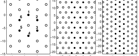
Figure 1: Formation of (a) photonic benzene, (b) benzene WG of $\pi-$type and (c) benzene WG of $\sigma-$type in a 2D hexagonal crystal; each solid dot denotes a defect atom of radius $\rho$.

$$<{\bf E}_{d}({\bf r})|{\epsilon}_{d}({\bf r})|{\bf E}_{d}({\bf r})>\stackrel{{\scriptstyle\mathrm{def}}}{{=}}\int_{domain}{\epsilon}_{d}({\bf r}){\bf E}_{d}({\bf r})\cdot{\bf E}_{d}({\bf r})d{\bf r}=1.$$

For the same photonic crystal considered in (1) but embedded with a photonic molecule, the allowed resonant modes are assumed as a superposition of the individual defect mode. Basically, it is analogous to the idea of LCAO, namely

$${\bf E}_{n}({\bf r})=\sum_{i=1}^{n_{d}}C_{ni}{\bf E}_{d}({\bf r}-{\bf R}_{i}),$$ (2)

where ${\bf E}_{n}({\bf r})$ is the nth resonant mode of the photonic molecule, $n_{d}$ the number of defect atoms, $C_{ni}$ the undetermined coefficient, and ${\bf R}_{i}$ the coordinates of the ith defect atom. Similarly, ${\bf E}_{n}({\bf r})$ satisfies (1) but with ${\epsilon}_{d}({\bf r})$ replaced by the dielectric constant ${\epsilon}_{pm}({\bf r})$ of the photonic molecule system, and $\omega_{d}$ replaced by the frequency $\omega_{n}$ of the eigenmode ${\bf E}_{n}({\bf r})$. That is

$$\hat{{\bf H}}{\bf E}_{n}({\bf r})={\epsilon}_{pm}({\bf r})(\omega_{n}/c)^{2}{\bf E}_{n}({\bf r}).$$ (3)

Equation (2) associated with (3) is a linear variational problem. Assigning different coefficient $C_{ni}$ to each mode $E_{d}$ may create different $E_{n}$, but the structure of photonic molecule will decide which resonant modes are allowed. This inference will be reflected on restricting $C_{ni}$ to satisfy the minimum of functional frequency, defined as

$$\Omega(C_{ni})\stackrel{{\scriptstyle\mathrm{def}}}{{=}}\frac{\left<{\bf E}_{n}({\bf r})\left|\hat{{\bf H}}\right|{\bf E}_{n}({\bf r})\right>}{\left<{\bf E}_{n}({\bf r})|{\epsilon}_{pm}({\bf r})|{\bf E}_{n}({\bf r})\right>}=\frac{\sum_{ij}C_{ni}C_{nj}{\bf H}_{ij}}{\sum_{ij}C_{ni}C_{nj}{\bf S}_{ij}}.$$

Namely, $\Omega$ is equivalent to the familiar Rayleigh-Ritz principle. Here ${\bf H}_{ij}$ and ${\bf S}_{ij}$ denote, respectively, the elements of the Hamiltonian matrix and the overlap matrix. According to (1) and (2), ${\bf H}_{ij}$ can be written as

$${\bf H}_{ij}=\left<{\bf E}_{d}\left({\bf r}-{\bf R}_{i}\right)\left|\hat{{\bf H}}\right|{\bf E}_{d}\left({\bf r}-{\bf R}_{j}\right)\right>$$

$$= \begin{cases}\left(\omega_{d}/c\right)^{2}={\alpha},\ \ \mbox{for $i=j$};\cr\left(\omega_{d}/c\right)^{2}\beta_{1},\ \mbox{for $(i,j)$ being the nearest-neighbor};\cr\left(\omega_{d}/c\right)^{2}\beta_{2},\ \mbox{for $(i,j)$ being the second-neighbor};\cr\left(\omega_{d}/c\right)^{2}\beta_{3},\ \mbox{for $(i,j)$ being the third-neighbor},\end{cases}$$

where $\beta_{(ij)}=<{\bf E}_{d}({\bf r}-{\bf R}_{i})|{\epsilon}_{d}({\bf r}-{\bf R}_{j})|{\bf E}_{d}({\bf r}-{\bf R}_{j})>$ denotes the hopping integral, whose magnitude measures the coupling strength and decays rapidly with increasing the distance $|{\bf R}_{i}-{\bf R}_{j}|$, i.e. $|\beta_{1}|>|\beta_{2}|>|\beta_{3}|$ (the more the defect sites split, the weaker their coupling ta ). Therefore, hopping terms can be classified according to the separation of the coupled defects. Here, only three relevant hopping terms are considered. Moreover, under the assumption that each individual defect mode is highly localized around its defect site, the field overlap between different defect atoms is small and the overlap integral ${\bf S}_{ij}$ can thus be approximated as

$${\bf S}_{ij}=<{\bf E}_{d}({\bf r}-{\bf R}_{i})|{\epsilon}_{pm}({\bf r})|{\bf E}_{d}({\bf r}-{\bf R}_{j})>\approx\delta_{ij}.$$ (4)

Now, vary $C_{ni}$ to minimize the functional frequency $\Omega$, with the necessary condition of ${\partial}\Omega/{\partial}C_{ni}=0$, $i=1,2,\dots,n_{d}$. One can obtain

$$\sum_{j=1}^{n_{d}}\left[{\bf H}_{ij}-\left(\omega_{n}/c\right)^{2}\delta_{ij}\right]C_{nj}=0.$$

The constrain of resonant frequencies can thus be derived from the solvability condition of $C_{ni}$. This leads to

$$\det\left[{\bf H}_{ij}-\left(\omega_{n}/c\right)^{2}\delta_{ij}\right]=0.$$ (5)

Equation (5) indicates that the allowed resonant frequencies in a given photonic molecule are dominated by hopping integrals. Furthermore, these hopping terms are dependent upon the dielectric structure of the photonic molecule. Therefore, every resonant mode is characterized by photonic molecule and exhibits different optical transmittance. To check the accuracy of Eq. (5), we first apply Eq. (5) to the photonic benzene, that yields

$$\left|\begin{matrix}{\alpha}-\gamma&\tilde{\beta}_{1}&\tilde{\beta}_{2}&\tilde{\beta}_{3}&\tilde{\beta}_{2}&\tilde{\beta}_{1}\cr\tilde{\beta}_{1}&{\alpha}-\gamma&\tilde{\beta}_{1}&\tilde{\beta}_{2}&\tilde{\beta}_{3}&\tilde{\beta}_{2}\cr\tilde{\beta}_{2}&\tilde{\beta}_{1}&{\alpha}-\gamma&\tilde{\beta}_{1}&\tilde{\beta}_{2}&\tilde{\beta}_{3}\cr\tilde{\beta}_{3}&\tilde{\beta}_{2}&\tilde{\beta}_{1}&{\alpha}-\gamma&\tilde{\beta}_{1}&\tilde{\beta}_{2}\cr\tilde{\beta}_{2}&\tilde{\beta}_{3}&\tilde{\beta}_{2}&\tilde{\beta}_{1}&{\alpha}-\gamma&\tilde{\beta}_{1}\cr\tilde{\beta}_{1}&\tilde{\beta}_{2}&\tilde{\beta}_{3}&\tilde{\beta}_{2}&\tilde{\beta}_{1}&{\alpha}-\gamma\end{matrix}\right|=0,$$ (6)

where we let $\gamma=(\omega_{n}/c)^{2}$ and $\tilde{\beta}_{i}=(\omega_{d}/c)^{2}\beta_{i}$ for simplification. The determinant in Eq. (6) is called the 6th-order circulant, and is equivalent to

$$\prod_{n=1}^{6}\left[\left({\alpha}-\gamma\right)+e_{n}\tilde{\beta}_{1}+e_{n}^{2}\tilde{\beta}_{2}+e_{n}^{3}\tilde{\beta}_{3}+e_{n}^{4}\tilde{\beta}_{2}+e_{n}^{5}\tilde{\beta}_{1}\right]=0,$$

where $e_{1},e_{2}\dots e_{6}$ are the six roots of unity, i.e. $e_{n}=exp(2\pi in/6)$. Hence, for $n=1\dots 6$, the frequencies $\omega_{n}$ of the six resonant modes ${\bf E}_{n}$ can be found as

$$\omega_{n}=\omega_{d}\sqrt{1+2\cos\frac{2\pi n}{6}\beta_{1}+2\cos\frac{2\pi n}{3}\beta_{2}+(-1)^{n}\beta_{3}}.$$ (7)

Obviously, Eq. (7) indicates that there are two doubly-degenerate frequencies with $n=1,5$ and $n=2,4$, and two nondegenerate frequencies with $n=3$ and $n=6$, thus, four high-Q resonant frequencies will occur within the major band gap. From the view point of the symmetry group , the photonic benzene belongs to the point group $C_{6v}$ for the 2D or $D_{6h}$ for the 3D systems, whose irreducible representation $\Gamma$ on defect sites can be reduced to the decomposition $\Gamma=A_{1}+B_{2}+E_{1}+E_{2}$ or $\Gamma=A_{2u}+B_{2g}+E_{1g}+E_{2u}$, respectively. Exactly speaking, it again illustrates two doubly degenerate modes of $E_{1}$ (or $E_{1g}$) and $E_{2}$ (or $E_{2u}$), and two nondegenerate modes of $A_{1}$ (or $A_{2u}$) and $B_{2}$ (or $B_{2g}$). Furthermore, these predictions are also consistent with the numerical solution of Eq. (3), that is calculated by scattering method (cf. ta ). The resultant transmission for the 2D case is plotted in Fig. 2, and the allowed resonant modes are shown in Fig. 3, where we consider a 2D finite-size hexagonal photonic crystal with a dielectric contrast ratio $8.4/1.0$ (rod/background) and a radius-to-spacing ratio $0.4/4.0$. The defect radius $\rho$ is taken as zero.

Figure 2 shows four nomalized resonant frequencies $0.369$, $0.375$, $0.455$ and $0.508$, that split from $\omega_{d}=0.419$ due to the defect coupling in a photonic benzene. By substituting these five frequencies into Eq. (7), the hopping terms $\beta_{1}$, $\beta_{2}$ and $\beta_{3}$ can be calculated by least-squares method, and they are $0.178$, $0.051$ and $-0.010$. Table I summarizes four cases of defect sizes, in which the all values of hopping parameters achieve the accuracy of two decimal places for Eq. (7). It clearly shows that the larger the defect radius is, the smaller hopping parameters. This means that the defect couplings in photonic benzene become weaker as the defect radius is increased. Moreover, when the defect radius $\rho$ is increased up to about $0.2$, the property of four transmission peaks disappeares, owing to that the shallow perturbation of dielectricity for defect atoms will create shallow modes ya0 .

Table 1: The calculated values of normalized resonant frequencies and hopping parameters for photonic benzene with different $\rho$.

$\rho$	$\omega_{d}$	$\omega_{1}$	$\omega_{2}$	$\omega_{3}$	$\omega_{4}$	$\beta_{1}$	$\beta_{2}$	$\beta_{3}$
0.0	0.419	0.455	0.375	0.369	0.508	0.178	0.051	-0.010
0.05	0.417	0.452	0.373	0.367	0.505	0.177	0.051	-0.009
0.1	0.409	0.442	0.369	0.361	0.493	0.171	0.048	-0.006
0.15	0.395	0.423	0.361	0.351	0.468	0.155	0.040	-0.002

In fact, Eq. (3) is equivalent to the effective Shr$\ddot{o}$dinger equation of H$\ddot{u}$ckel $\pi-$electron theory (developed in 1931 hu ), if we make the resonant modes of 3D photonic benzene be analogous to the $\pi-$electrons of benzene molecule. However, Eq. (3) is much simpler. Theoretically, the $\pi$-electrons arise from a planar unsaturated organic molecule whose MOs can be divided into the $\sigma$ and $\pi$ MOs according to the reflection symmetry in the molecular plane. Both systems belong to the same point group $D_{6h}$ and have the same degeneracy (cf. at , p.261), but possess completely different meanings. Conceptually, the photonic molecule acts as a perfect model of artificial molecule, since the resonant modes are much easier to be realized than the bonding orbitals of real molecule. Similar phenomena can also be found in the quantum-dot molecules pi or the coupled pairs of GaAs cavities (note that these systems are also termed as photonic molecule, cf. Bayer et al. bayer ). Fig. 3 shows the lowest resonant modes allowed in a 2D photonic benzene with $\rho=0.0$, and they are labelled according to the symmetry species of the group $C_{6v}$, which are analogous to the six $\pi$ MOs of benzene molecule but is lacking of the $C_{1h}$ symmetry.

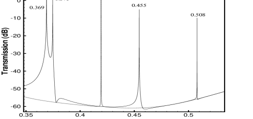
Figure 2: Transmission amplitude of electric field as function of normalized frequency for a photonic benzene (solid curve) and a defect atom (dotted curve). The marked values are four frequencies of the high-Q modes which are split from the $\omega_{d}$ due to defect coupling and fallen in the major band gap whose rang is as shown in Fig 4.

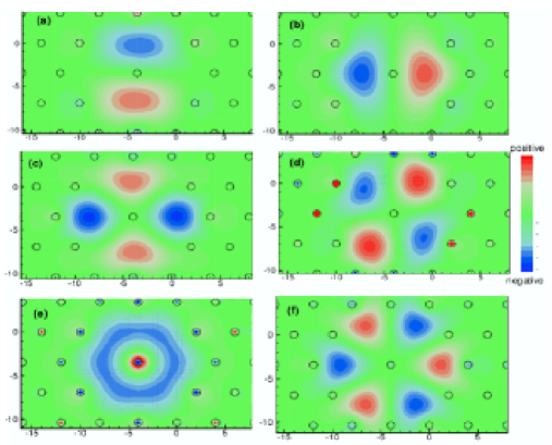
Figure 3: Resonant electric field pattern in a photonic benzene of $\rho=0$ for the six lowest resonant modes with normalized frequencies of (a) 0.369 with $E_{1}$ mode, (b) 0.369 with $E_{1}$ mode, (c) 0.455 with $E_{2}$ mode, (d) 0.455 with $E_{2}$ mode, (e) 0.375 with $A_{1}$ mode and (f) 0.508 with $B_{2}$ mode, respectively. In general, the more node, the higher frequency.

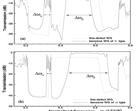
Figure 4: Transmission created by benzene WGs of (a) $\pi-$type and (b) $\sigma-$type with $\rho=0.0$. Both types present the feature of twin waveguiding bandwiths, marked as $\triangle\omega_{{\alpha}}$ and $\triangle\omega_{\beta}$.

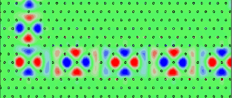
Figure 5: Eletric field distribution of a TM light with $E_{2}$ mode travels through a $90^{o}$ bend in a benzene WG where the junction connects a $\pi$ type WG with a $\sigma$ type; incident wave with normalized frequencies 0.449 enters from the upper left.

Most importantly, by applying the modular concept of photonic benzene can create photonic WGs, and we called these WGs as benzene WGs. In the chemistry terminology, benzene WGs can be classified as $\pi$ and $\sigma$ types corresponding to the bonding types between two real benzene rings, as illustrated in Fig. 1 (b) & (c). It is remarkable that transmission of the benzene WGs reveals the special feature of a twin waveguiding bandwidths marked as $\triangle\omega_{{\alpha}}$ and $\triangle\omega_{\beta}$, where $\triangle\omega_{{\alpha}}<\triangle\omega_{\beta}$, as shown in Fig. 4. This means that the benzene WGs are able to provide two working bandwidths at the same time. In addition, Fig. 5 shows that a TM light with the $E_{2}$ mode travels through a $90^{o}$ bend from the $\pi$ type to the $\sigma$ type. Of course, the same phenomenon can also be observed in other modes.

In conclusion, we suggest a new and practicable idea for the manipulation of photonic defects, that includes the so-called photonic molecule and benzene WG. The optical properties of photonic molecules has been investigated by variational theory, which shows that the allowed resonant frequencies inside a photonic molecule are dominated by hopping parameters through the constraint (5). Taking the photonic benzene as an example, six resonant modes with two doubly-degenerate and two nondegenerate are found and verified by both of the scattering method and group theory. Especially, the benzene WGs created by the modular manipulation of photonic benzenes are demonstrated to possess the interesting feature of a twin waveguiding bandwidths. Namely, benzene WGs provide two working bandwidths at the same time and make the function of guiding photons more flexible.

This work is supported in part by the Global Fiberoptics, Inc.

References

- (1) E. Yablonovitch, T. J. Gmitter, R. D. Meade, A. M. Rappe, K. D. Brommer, and J. D. Joannopoulos, Phys. Rev. Lett. 67, 3380 (1991).
- (2) E. , G. Tuttle, M. Sigalas, C. M. Soukoulis, and K. M. Ho, Phys. Rev. B51, 13961 (1995).
- (3) P. R. Villeneuve, S. Fan, and J. D. Joannopoulos, Phys. Rev. B54, 7837 (1996).
- (4) A. Mekis, J. C. Chen, I. Kurland, S. Fan, P. R. Villenuve, and J. D. Joannopoulos, Phys. Rev. Lett. 77, 3787 (1996).
- (5) A. Mekis, S. Fan, and J. D. Joannopoulos, Phys. Rev. B58, 4809 (1998).
- (6) S. Y. Lin, E. Chow, V. Hietala, P. R. Villenuve, and J. D. Joannopoulos, Science 282, 274 (1998).
- (7) S. Boscolo and M. Midrio, Opt. Lett. 27, 1001 (2002).
- (8) A. Yariv, Y. Xu, R. K. Lee, and A. Scherer, Opt. Lett. 24, 711 (1999).
- (9) M. Bayindir, B. Temelkuran, and E. Ozbay, Phys. Rev. Lett. 84, 2140 (2000).
- (10) M. Bayindir, B. Temelkuran, and E. Ozbay, Phys. Rev. B61, R11855 (2000).
- (11) H. Kosaka, T. Kawashima, A. Tomita, M. Notomi, T. Tamamura, T. Sato, and S. Kawakami, Appl. Phys. Lett. 74, 1370 (1999).
- (12) A. R. McGurn, Phys. Rev. E65, 075406 (2002).
- (13) E. Lidorikis, M. M. Sigalas, E. N. Economou, and C. M. Soukoulis, Phys. Rev. Lett. 81, 1405 (1998).
- (14) K. M. Leung, J. Opt. Soc. Am. B 10, 303 (1993).
- (15) J. P. Albert, C. Jouanin, D. Cassagne, and D. Bertho, Phys. Rev. B61, 4381 (2000).
- (16) A. Garcia-Martin, D. Hermann, K. Busch, and P. Wlfle, Mat. Res. Soc. Symp. Proc. 722, L 1.1.1 (2002).
- (17) G. Tayeb and D. Maystre, J. Opt. Soc. Am. A 14, 3323 (1997).
- (18) E. Hckel, Z. physik 70, 204 (1931).
- (19) P. W. Atkins and R. S. Friedman, Molecular Quantum Mechanics (Oxford University, Oxford, 1997).
- (20) M. Pi, A. Emperador, M. Barranco, F. Garcias, K. Muraki, S. Tarucha, and D. G. Austing, Phys. Rev. Lett. 87, 066801 (2001).
- (21) M. Bayer, T. Gutbrod, J. P. Reithmaier, A. Forchel, T. L. Reinecke, P. A. Knipp, A. A. Dremin and V. D. Kulakovskii, Phys. Rev. Lett. 81, 2582 (1998).