Using data assimilation in laboratory experiments of geophysical flows

Data assimilation is used in numerical simulations of laboratory experiments in a stratified, rotating fluid. The experiments are performed on the large Coriolis turntable (Grenoble, France), which achieves a high degree of similarity with the ocean, and the simulations are performed with a two-layer shallow water model. Since the flow is measured with a high level of precision and resolution, a detailed analysis of a forecasting system is feasible. Such a task is much more difficult to undertake at the oceanic scale because of the paucity of observations and problems of accuracy and data sampling. This opens the way to an experimental test bed for operational oceanography. To illustrate this, some results on the baroclinic instability of a two-layer vortex are presented.

1 Introduction : operational issues

An increasing interest in operational oceanography has developed in recent years. A number of pre-operational projects have emerged at the national and international scale, most of them coordinating their activites within the international Global Ocean Data Assimilation Experiment (GODAE).

The heart of operational systems consists of three main components : the observation system, the dynamical model and the data assimilation scheme. Thanks to recent advances in satellite and in-situ observations, numerical modelling, assimilation techniques and computer technology, the operational systems have now acquired some degree of maturity. However, there are still a number of issues that must be solved in applications, and validation tests are needed.

The ideal method for validating the overall forecasting system would be to compare results with independent oceanic observations, i.e. observations that are not used in the assimilation process. However, such observations are rare because in-situ surveys are difficult to undertake and extremely expensive, particularly in the deep ocean. Another problem is that, because assimilation is only approximate, forecast errors may be due not only to the model itself, but also to the temporal growth of imperfections in the initial condition. It is therefore difficult to objectively identify the model errors on the one hand and the assimilation errors on the other.

Alternatively, analytical solutions of simple flows with well-defined initial and boundary conditions can be used as a reference to unravel some aspects of the model error components. However, such analytical solutions are limited to some extremely simplified flow configurations.

In this letter, a new, experimental approach to these problems is presented. Laboratory experiments and numerical, shallow water simulations of simple oceanic flows are performed and sequential data assimilation is used as a tool to keep the numerical simulation close to the experimental reality. By contrast with real-scale oceanic measurements, the experimental measurements are available with a high level of precision and resolution. The general methodology is given in Section 2. In Section 3, the example of un unstable vortex in a two-layer, rotating fluid is presented as an illustration of the experimental test-bed. In particular, the behaviour of the model is studied when data assimilation is stopped. The vortex deformation and splitting as predicted by the numerical simulation is then compared to the real flow evolution.

2 The Coriolis test-bed

Laboratory experiments are of particular interest as test cases for operational systems, filling the gap between the oversimplified analytical solutions and the full complexity of real oceans. On the one hand, they are much more realistic than any numerical or theoretical “reality”, provided that the experimental facility allows good similarity with the ocean. On the other hand, data are available with much better space and time resolution than actual scale oceanic measurements. Furthermore, a great number of experiments can be performed and compared to one other. Such comparisons are obviously impossible at the real scale because of the ever changing flow conditions in the ocean. The flow parameters can also be easily varied to perform parametric studies.

Thanks to its large size (13 meter diameter), the Coriolis turntable (Grenoble, France) is a unique facility which enables oceanic flows to be reproduced with a good level of similarity (see Fig.1). It is possible to come close to inertial regimes, i.e. with limited effects of viscosity and centrifugal forces. Various experiments can be performed on the turntable in multi-layer stratified salt water, such as experiments on vortices or boundary currents.

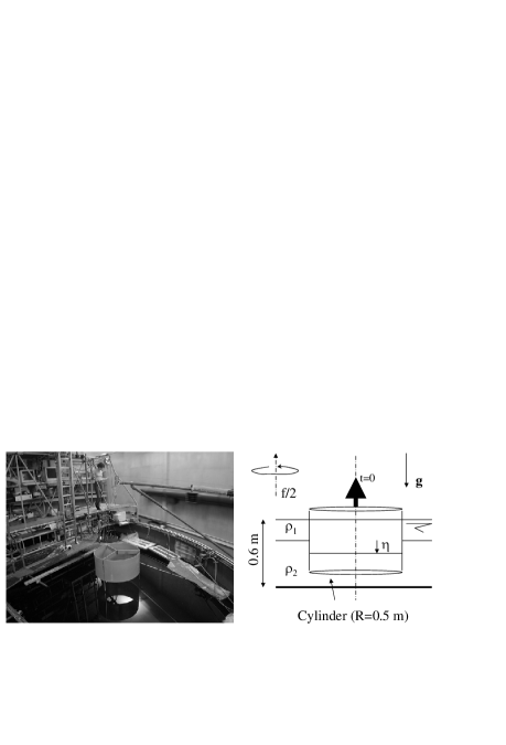
Figure 1: Picture of the Coriolis turntable with the setup of the two-layer vortex experiment. The layers have density $\rho_{1}$ and $\rho_{2}>\rho_{1}$ and undisturbed thickness $H_{1}$=12.5 cm and $H_{2}$=50 cm. For the experiment presented in this paper, the relative density difference is 1.0 10^-3, the initial displacement of the interface is $\eta_{0}=-H_{1}$ inside the cylinder, and the tank rotation period is 40 s. The corresponding Rossby radius of deformation is 12.5 cm. At $t=0$ the cylinder is removed.

Our approach relies on numerical simulation of such laboratory experiments using data assimilation, in a similar way to real-scale ocean forecasting systems. A major difference with the real ocean is that the measured quantity here is the velocity field in several horizontal planes instead of scalar quantities measured only at the surface or along vertical sections. The elevation of the interface between the layers is not measured in the experiments. It is treated as an output of the asssimilation process (see section 3).

The velocity field is measured in horizontal planes using CIV (Correlation Image Velocimetry): particle tracers are illuminated by a horizontal laser sheet and a camera is used to visualize the particle displacements from above, leading, after numerical treatment, to the horizontal velocity field. The rms measurement error in particle displacement is about 0.2 pixels, as determined by Fincham & Delerce (2000), and the errors found in neighboring points are not correlated. The resulting error in velocity about 3% of the maximum velocity.

In parallel with these measurements, numerical simulations are performed. The system is modelled as a multi-layer fluid with hydrostatic approximation for which the variables are the horizontal velocity components $u(x,y,i)$ and $v(x,y,i)$, and the layer thickness $h(x,y,i)$, where $x$ and $y$ are the horizontal coordinates and $i$ is the layer index. The basic shallow-water equations are solved using MICOM (Miami Isopycnic Coordinate Ocean Model, Bleck & Boudra 1986) in its simplest version.

The measured velocity field is assimilated into the simulations at each measurement point using an adaptive version of the Singular Evolutive Extended Kalman (SEEK) filter, a method adapted for oceanographic purposes on the basis of the Kalman filter. Each data assimilation provides a new dynamical state which optimally blends the model prediction and the measured data, in accounting for their respective error. The forecast state vector ${\textbf{X}}^{f}$ is replaced by the analysed state vector ${\textbf{X}}^{a}={\textbf{X}}^{f}+{\textbf{K}}[{\textbf{Y}}^{o}-{\textbf{H}}{\textbf{X}}^{f}]$ ,where ${\textbf{Y}}^{o}$ is the observed part of the state vector (i.e. the velocity field in the measurement domain), H is the observation operator and K is the Kalman gain defined by ${\textbf{K}}={\textbf{P}}^{f}{\textbf{H}}^{T}\;[{\textbf{H}}{\textbf{P}}^{f}{\textbf{H}}^{T}+{\textbf{R}}]^{-1}$. Here, ${\textbf{P}}^{f}$ and R are the forecast error and observation error covariance matrices respectively. The observation errors are here supposed to be uniform, and the multi-variate correlations between the variables are described as components on Empirical Orthogonal Functions (EOF’s) computed from the model statistics, providing an estimation of ${\textbf{P}}^{f}$. The reader is referred to Pham, Verron & Roubaud (1998) and Brasseur, Ballabrera-Poy & Verron (1999) for mathematical details.

3 Example : Baroclinic instability of a two-layer vortex

Among the various experiments performed on the Coriolis turntable, concerning, for example, baroclinic instability and coastal currents, the study of the baroclinic instability of a two-layer vortex is presented in the present letter because it provides a good illustration of the experimental test-bed. This flow problem is of particular interest because simple experiments are feasible as well as numerical simulations, although it is quite a complex non-linear process (e.g. Griffiths and Linden 1981) and plays a crucial role in the variability of the real ocean. The initial conditions are well defined and the lateral boundaries have no significant influence.

A cylinder of radius $R=$ 0.5 m is initially introduced in a two-layer fluid across the interface (see Fig. 1). A displacement $\eta_{0}$ of the interface is produced inside the cylinder, and at $t=0$ the cylinder is rapidly removed. A radial gravity current is then initiated, which is deviated by the Coriolis force, resulting in the formation of a vortex in the upper layer after damping of inertial oscillations. A vortex of opposite sign is produced in the lower layer, and the resulting vertical shear is a source of baroclinic instability. The main control parameter in this system is $\gamma=R/R_{D}$, where $R_{D}$ is the Rossby deformation radius. The results presented here were obtained with $\gamma=4$. The vortex then undergoes baroclinic instability which gives rise to splitting into two new vortices.

The experimental vortex is dynamically similar to an oceanic vortex with a radius of the order of $100$ km at mid-latitude (the radius of deformation is typically 25 km). In the experiments, vortex instability takes place in typically 20 rotation periods of the tank, corresponding to about 30 days at mid-latitude (taking the inverse of the Coriolis parameter as the relevant time unit). The ratio of the vertical to the horizontal scales is distorted by a factor of 10 in the experiments. This is not important provided that the hydrostatic approximation is valid.

The velocity field is measured in each layer every 11 s, which is half the observed period of inertial oscillations. Since we are interested in the slow balanced dynamics, we eliminate the residual inertial oscillations by averaging two successive fields for data assimilation. The velocity data obtained are assimilated in the numerical model at each grid point in the measurement domain (2.5 m $\times$ 2.5 m). In the numerical simulations, the system is modelled as a two-layer fluid with a standard biharmonic dissipation term and the simulation domain is 5 m wide (i.e. twice as large as the measurement domain) in order to avoid spurious confinement by boundaries. The simulations are performed using 100² or 200² grid points in each layer.

A good fit is then obtained between the model and the experimental data, as shown in Fig. 2. The irregular shape of the vortex, the position of its center and the presence of residual currents in its vicinity are well represented. The elongation of the vortex and the formation of two new, smaller vortices are also well reproduced. Data assimilation provides us with an indirect measurement of the interface depth, also shown in Fig. 2. No significant inertio-gravity wave is excited in the simulation after data assimilation is performed, showing that the interface position is well determined, without any spurious imbalance effect.

The initial development of baroclinic instability is well described by the growth of mode two (calulated using a polar Fourier decomposition of the radial velocity field along a circle of radius R). Excellent agreement between the model and the observation is obtained when data assimilation is performed, as shown in Fig. 3. The growth of this mode is considerably delayed in the model without data assimilation, as the initial perturbation is smaller than in the experiments.

The rms distance between the forecast and measured velocity fields is plotted in Fig. 4. After a few assimilation cycles, this distance remains of the order of 0.6 mm.s^-1, close to the experimental errors (3% of the maximum velocity, i.e. about 0.5 mm.s^-1). Similar agreement is obtained in both layers.

The state vector obtained at a given time can be used as an initial condition to test the free model. To do so, we stop the assimilation at time $t=75s$ and measure the growth of the rms distance between the laboratory experiments and the free model run with this new initial state, as shown in Fig. 4. This growth can be due either to the amplification of small initial errors, or to limitations of the dynamical model. It is actually possible to show that the sensitivity to the initial condition is not the dominant effect, as observed in Fig. 5. It is clear in this figure that the divergence of the model from the experimental reality is not sensitive, over the short term, to small variations in the initial condition. The model diverges from reality on a timescale of around 3000s, which is about 30 times the typical advection timescale of the flow $2R/U\simeq 100s$ (where $U\simeq 1$ cm.s^-1 is the order of magnitude of the velocity within the flow). The model error is therefore about $1/30$ of the dominant advective term. This error is actually small but seems to be systematic.

The results are similar when 100² or 200² numerical grid points are used in each layer (see Fig. 4, 5 and 6). The effect of dissipation and friction was also investigated in various test runs. The rms distance to observations obtained in the most representative of these test runs is plotted in Fig. 4. The results show that the model errors persist when the numerical viscosity coefficient is changed or when an Ekman friction term is added in the momentum equation. We notice that, in all cases, vortex splitting occurs faster than in the experimental reality (Fig. 6). It is therefore likely that the basic simplifying assumptions of the hydrostatic, two-layer shallow-water formulation, rather than resolution, dissipation or friction problems, are responsible for the limitations of the model. For instance, the interface between the layers may have a finite thickness in reality, leading to effects that cannot be reproduced in the two-layer simulation. Also, the hydrostatic approximation may slightly enhance the growth of baroclinic instability, as shown in the theoretical study of non-hydrostatic effects by Stone (1971).

In the last stage of our testing procedure, we perform assimilation using only upper layer data and check how the behavior of the lower layer is reconstructed. The results are shown in Fig. 6. Although some local discrepancies are observed in the bottom layer compared to the measured velocity field, the global flow field is well reproduced.

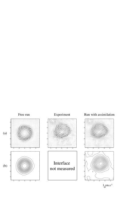
Figure 2: Velocity field in the top layer (a) and interface depth (b) at $t=75s$ in the free run, in the experiment and in the simulation performed with data assimilation every 22s. For clarity, only 25² vectors are plotted. The rms measurement error is about 0.5 mm.s^-1.

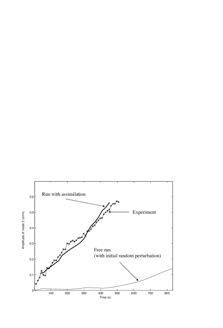
Figure 3: Amplitude of baroclinic mode 2 in the top layer as a function of time in the experiment (line with stars), in the free simulation (thin line) and in the simulation performed with data assimilation every 22s (thick line).

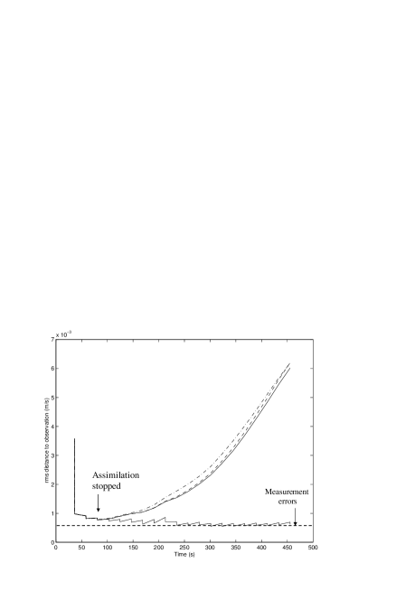
Figure 4: Value of the rms distance between the simulated and measured velocity fields in the top layer as a function of time in the simulation performed with data assimilation every 22s and in the simulation where data assimilation is stopped at $t=75s$. 200² grid points are used in both layers. The results obtained in two other test runs are also plotted : simulation with doubled viscosity coefficient (dashed line) and simulation with additional friction (dot-dashed line). The Ekman friction coefficient $C_{f}$ is taken as equal to $1.4\;10^{-3}s^{-1}$ in the bottom layer and $5.6\;10^{-3}s^{-1}$ in the top layer. These values are those obtained assuming rigid upper and lower boundaries.

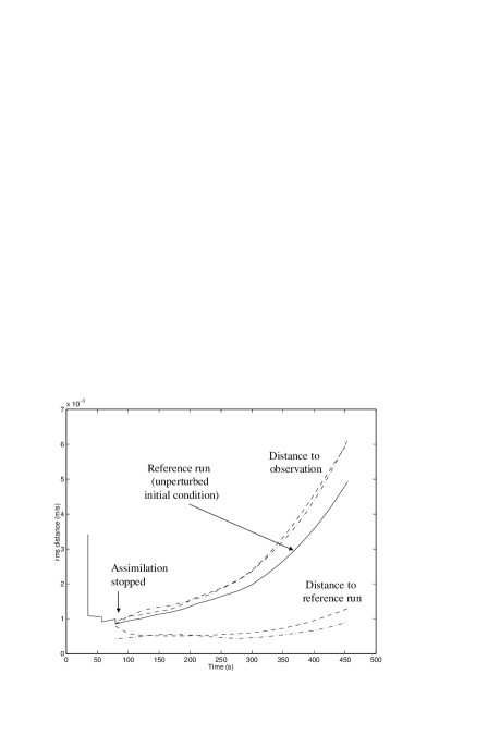
Figure 5: Value of the rms distance between the simulated and measured velocity fields in the top layer as a function of time when assimilation is stopped at $t=75s$. 100² grid points are used in both layers. Two test runs were performed using a perturbed initial condition at time $t=75s$. In the first test run (dashed line), the velocity field $\bf{u}$ in each layer is replaced at time $t=75s$ by $\bf{u}_{obs}+\bf{R}\;(\bf{u}-\bf{u}_{obs})$, where $\bf{u}_{obs}$ is the observed velocity field and $\bf{R}$ is the 90^o rotation operator. In the second test run (dot-dashed line), a large friction coefficient is imposed ($C_{f}=1.4\;10^{-2}s^{-1}$ in the bottom layer and $5.6\;10^{-2}s^{-1}$ in the top layer) from $t=0$ to $t=75s$ only, resulting in a slightly perturbed initial condition at time $t=75s$.

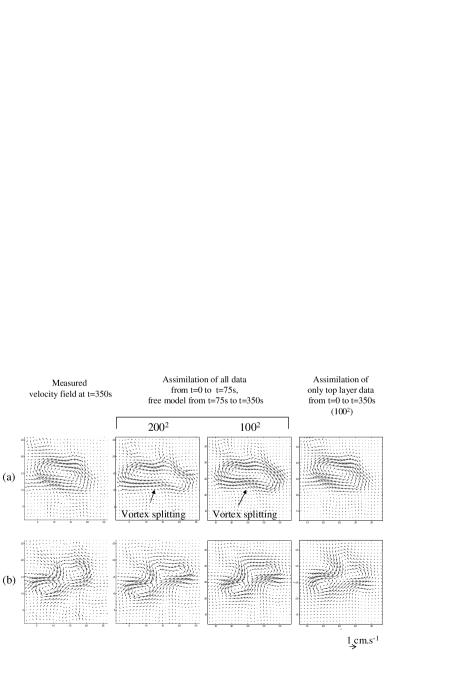
Figure 6: Velocity field in the top (a) and bottom (b) layers at $t=350s$ obtained in the experiment and in the simulation using different assimilation scenarios : assimilation of all data swithched off at $t=75s$ (note that the vortex splitting occurs faster than in the experiment, independently of the resolution); assimilation using only top layer data until $t=350s$ (note that the bottom layer is well reconstructed). For clarity, only 25² vectors are plotted in all cases.

4 Conclusion

The results reported in the present letter illustrate the interest of an experimental test-bed for operational oceanography :

(i) Thanks to data assimilation, a complete description of the experimental flow fields is obtained, including the non-measured variables. Any physical quantity can then be calculated. Data assimilation can thus be used as a complementary tool for experimental investigation and physical analysis of the flow. For instance, potential vorticity anomalies can be calculated, providing quantities which are generally impossible to measure but which are crucial to a better understanding of the physics of the baroclinic instability.

(ii) The obtained flow field can be used as an initial condition to test the numerical model. The divergence of the numerical model from reality is, in principle, caused either by the sensitivity of system evolution to the initial condition, or by the model error itself. We have checked that, in our test cases sensitivity to weak variations in the initial condition is not the dominant effect. This makes it possible to quantify the systematic forecast errors. Thus, even weak model errors can be detected, of the order of 1/30 of the dominant inertial term in the present case. Such a weak model limitation would be probably much more difficult to detect in complex oceanic applications. Test runs were performed to show that these model errors are not caused by resolution, dissipation or friction problems. The most probable sources of error are the hydrostatic approximation or the two-layer formulation of the equations. Further work is needed to test this hypothesis.

(iii) The accuracy of the assimilation scheme can also be analysed in detail. The present study shows, for instance, how the assimilation scheme is able to reconstruct the velocity field of the lower layer from observation of the upper layer. This is clearly of practical interest because vertical extrapolation of the measured surface quantities is a great challenge in oceanography (see for instance Hurlburt 1986).

Many other tests can of course be performed with the available data using various dynamical models and/or assimilation schemes. Possible improvement by non-hydrostatic models would be of particular interest. The study of other processes is in progress, involving the instability of boundary currents, gravity currents on a slope and current/topography interaction. The measurements obtained from these experiments are available to other researchers on the Coriolis web site (www.coriolis-legi.org) as a data base to test numerical models and assimilation schemes.

This study has been sponsored by EPSHOM, contract Nr. 9228. We acknowledge the kind support of Y. Morel for the implementation of the MICOM model, and of J.M. Brankart, P. Brasseur and C.E. Testut for the implementation of the SEEK assimilation scheme.

References

- [1] Bleck, R. and Boudra, D. Wind driven spin-up in eddy-resolving ocean models formulated in isopycnic coordinates, J. Geophys. Res., 91, 7611–7621, 1986.
- [2] Brasseur, P., Ballabrera-Poy, J. & Verron, J. 1999. Assimilation of altimetric data in the mid-latitude oceans using the Singular Evolutive Extended Kalman filter with an eddy-resolving, primitive equation model, J. Marine Sc. 22, 269–294, 1999.
- [3] Fincham, A. and Delerce, G. Advanced optimization of correlation imaging velocimetry algorithms, Experiments in Fluids 29, S13-S22, 2000.
- [4] Griffiths, R.W. and Linden, P.F. The stability of vortices in a rotating, stratified fluid. J. Fluid Mech. 105, 283-316, 1981.
- [5] Hurlburt, H.E. Dynamic Transfer of Simulated Altimeter Data Into Subsurface Information by a Numerical Ocean Model. J. Geophys. Res. 91, C2, 2372-2400, 1986.
- [6] Pham, D., Verron, J. and Roubaud, M. A Singular Evolutive Extended Kalman filter for data assimilation in oceanography, J. Marine Sc., 16 (3-4), 323–340, 1998.
- [7] Stone, P.H. Baroclinic instability under non-hydrostatic conditions. J. Fluid Mech. 45, part 4, 659-671, 1971.