Quantum Zeno Features
of Bistable Perception

Abstract

A generalized quantum theoretical framework, not restricted to the validity domain of standard quantum physics, is used to model the dynamics of the bistable perception of ambiguous visual stimuli. The central idea is to treat the perception process in terms of the evolution of an unstable two-state quantum system, yielding a quantum Zeno type of effect. A quantitative relation between the involved time scales is theoretically derived. This relation is found to be satisfied by empirically obtained cognitive time scales relevant for bistable perception.

1 Introduction

Quantum theory has revolutionized our understanding of the physical world in both scientific and epistemological respects. It was developed in the third decade of the $20^{\rm th}$ century as a theory describing the behavior of atomic systems. Subsequently, its range of validity turned out to be much wider. Not only are nuclei and elementary particles, more than seven orders of magnitude smaller than atomic systems, governed by quantum theory, but also macroscopic phenomena like superconductivity or superfluidity are successfully described in quantum theoretical terms.

¿From the present state of knowledge, the broad validity of quantum theory in physics is not surprising. Investigations of its conceptual structure and axiomatic foundations have revealed that quantum theory is a logical consequence of some rather simple and plausible basic assumptions on the nature of observables and states of physical systems. In this framework, classical physics results from basically one additional assumption: the commutativity of the algebra of observables. On the other hand, the axiomatic framework has shown how deeply rooted apparently bizarre concepts of quantum theory like complementarity and entanglement really are, and that there is no way back to classical concepts on a fundamental level of physical description.

Since the early days of quantum theory, starting with Niels Bohr, the idea has been entertained that quantum theoretical concepts like complementarity and entanglement might be meaningful and important even beyond the realm of the physical world in its strict sense. Concerning such “quantum-like” phenomena, encorporating complementarity or entanglement beyond physics, three different stances, not completely exclusive with respect to each other from a logical point of view, are possible and have found proponents.

1. The application of quantum theoretical concepts to non-physical situations is merely metaphoric and not elucidated in a precise and general way. The analogies are selected ad hoc and change with the given situation.

2. In the spirit of a strict physicalism, everything can be reduced to physics. There is nothing left beyond the world of physics, and quantum-like phenomena as adressed above are simply physical quantum phenomena.

3. Assuming a non-reductive framework, it might be possible and adequate to describe vital features of parts of the world, physical or non-physical, by a formalism isomorphic to the formalism of quantum theory. This isomorphy may be total or, more often, partial, such that only particular features of the quantum theoretical formalism are realized in a non-physical context.

An approach within option (3), denoted as weak quantum theory, was recently proposed on an axiomatic basis [2]. The starting point in this approach is the algebraic formulation of quantum theory, where the observables of a physical system generate a $C^{*}$-algebra $\cal{A}$, and the states of the system are positive linear functionals on $\cal{A}$. A careful analysis of this formulation shows that its axioms are not equally fundamental. They can be sifted out into general, indispensable axioms, applying to any (physical or non-physical) system as long as it is a possible object of meaningful investigation, and more special axioms used in quantum physical applications only.

The most general formal system thus arising, in which concepts like complementarity and entanglement are still meaningful, is a minimal version of weak quantum theory. In short, it can be described in the following way (for details we refer to [2]):

The notions of system, observables, and states remain unchanged. Observables are identified with functions mapping states to states. This emphasizes the importance of observables as representing active processes with the capacity of changing states, which is vital in quantum theory.

Observables, conceived as functions, can be composed. This composition defines a multiplication of observables endowing the set of all observables with the simple structure of a semigroup. Two observables are incompatible, or complementary with respect to each other, whenever they do not commute. Entanglement can be rephrased as complementarity of a global observable pertaining to a system as a whole and local observables pertaining to its parts. Propositions are special observables related to yes-no-questions about the system.

The minimal, most general formal system of weak quantum theory can be stepwise supplemented and enriched up to isomorphy with the full quantum theory used in physics. In its minimal form, weak quantum theory, although it implies complementarity and entanglement, is vastly more general and flexible than the full quantum theory. The main differences are:

• In the most general form of weak quantum theory, the sum of observables is not defined in an empirically meaningful way. As a consequence, there is no Hilbert space of states and no way to attribute probabilities to the outcomes of measurements corresponding to the observables.

• Planck’s constant $h$, which determines the amount of non-commutativity and complementarity in quantum physics, enters nowhere. This implies that conspicuous quantum-like phenomena may be effective in situations beyond standard quantum physics.

• Unlike in quantum theory, where Bell’s inequalities can be derived, there is in general no way to rule out local realism. As a consequence, indeterminacies and complementarities can be of epistemic rather than ontic origin.

Quantum-like behavior as described by weak quantum theory or its refinements is expected for systems with complex internal organization. This implies strong and intricate coupling of their parts and the practical impossibility of observation from outside without influencing the state of such systems.

A paradigmatic example for such a situation is the cognitive system and its neural correlates in the brain. This may be one of the reasons why quite a number of approaches have been developed, in more or less detail, to relate conscious activities to quantum theory or describe particular brain operations quantum theoretically. Besides the fairly popular approaches associated with the names of von Neumann/Wigner/Stapp [31] and Penrose/Hameroff [22], other interesting options have been proposed by Beck/Eccles [4] and Umezawa/Vitiello [29].

All these approaches are essentially discussed within the usual quantum physics. This is at variance with the strategy of weak quantum theory; a recently discussed example refers to the perception of temporally subsequent events [3]. This approach proposes a type of temporal entanglement which is not contained in standard quantum physics, but can be formulated in the theory of chaotic systems. In the present paper, we intend to apply the framework of weak quantum theory to another scenario of cognitive science: the bistable perception of ambiguous stimuli.

Bistable perception arises whenever a stimulus can be interpreted in two different ways with approximately equal plausibility. A very simple and often investigated example of bistable perception is the so-called Necker cube. (For an overview concerning the current discussion of cognitive and neural features of the perception of the Necker cube see [14, 15].) A grid of a cube in two-dimensional representation can be perceived as a three dimensional-object in two different perspectives, either as a cube seen from above or from below. The perception of the Necker cube switches back and forth between the two possible interpretations spontaneously and inevitably.

We propose to describe bistable perception with the formalism of a two-state quantum system, where the two basis states correspond to the two different ways to interpret the visual stimulus. Measurement is considered as the mental process determining in which way the figure is perceived. The switching between the different perceptions corresponds to the quantum transition between the two states which are eigenstates of the operator representing a particular perception and unstable under the time evolution of the system.

Such a description of bistable perception employs a non-minimal version of weak quantum theory with a linear structure and a two-dimensional linear state space. This version is fairly close to the structure of the full quantum theory used in physics. This does not imply, however, that we propose to understand bistable perception as a quantum phenomenon in the sense that the related brain processes are usual quantum processes. (Planck’s constant $h$ will nowhere enter in our arguments.) Rather, we will discuss the quantum-like behavior of bistable perception as a result of the truncation of an extremely complicated system to a two-state system, into which the effect of many uncontrolled variables and influences is lumped in a global way.

For this purpose, we consider a quantum mechanical system with a state space spanned by two states $\psi_{1}$ and $\psi_{2}$, neither of which is an eigenstate of the Hamiltonian $H$ generating the evolution matrix $U(t)={\rm e}^{{\rm i}Ht}$. If the system is initially in the state $\psi_{1}$ and allowed to evolve freely according to $U(t)$, then its state will oscillate between the states $\psi_{1}$ and $\psi_{2}$. This oscillation can be slowed down by increasing the frequency at which the system is measured, asking whether it still resides in its initial state. In the limit of continuous measurement, the evolution of the system can be completely suppressed. This phenomenon is known as the quantum Zeno effect.

In the following section 2, the quantum Zeno effect will be described in as much detail as required for the purpose of this paper. The quantitative relation between different time scales of crucial significance will be emphasized in particular. In section 3, cognitive time scales satisfying this relation will be presented with particular respect to the dynamics of bistable perception. Section 4 summarizes the results and concludes the article.

2 Quantum Zeno effect

The quantum Zeno effect was originally discussed as the quantum Zeno “paradox” by Misra and Sudarshan [19] for the decay of unstable quantum systems. As mentioned above, its key meaning is that repeated observations of the system decelerate the time evolution which it would undergo without observations, e.g. its decay. The metaphor “a watched pot never boils” paraphrases this behavior in the limit of continuous observation.

The situation addressed in the following refers to a quantum system oscillating between two non-stationary states. For this purpose, we consider a system with the following properties:

1. For convenience, a two-state system will be considered. (The results apply to more general systems as well.)

2. An observation is represented by the operator

   $$\sigma_{3}=\left(\begin{array}[]{cc}1&0\\ 0&-1\end{array}\right).$$

   Immediately after an observation, the system will be in one of the corresponding eigenstates

   $$\psi_{1}=|+\rangle=\left(\begin{array}[]{c}1\\ 0\end{array}\right)\hskip 28.45274pt{\rm or}\hskip 28.45274pt\psi_{2}=|-\rangle=\left(\begin{array}[]{c}0\\ 1\end{array}\right).$$

3. Both $\sigma_{3}$-eigenstates may also be represented by their projection operators

   $$P_{+}=\left(\begin{array}[]{cc}1&0\\ 0&0\end{array}\right)\hskip 28.45274pt{\rm and}\hskip 28.45274ptP_{-}=\left(\begin{array}[]{cc}0&0\\ 0&1\end{array}\right).$$

4. Without loss of generality, the Hamilton operator giving rise to transitions of the system can be written as

   $$H=g\sigma_{1}=g\left(\begin{array}[]{cc}0&1\\ 1&0\end{array}\right),$$

   where $g$ is a coupling constant. Hence, the unitary operator of time evolution is represented by

   $$U(t)={\rm e}^{{\rm i}Ht}=\left(\begin{array}[]{cc}\cos gt&{\rm i}\sin gt\\ {\rm i}\sin gt&\cos gt\end{array}\right).$$

5. In this model, $\Delta T$ defines the time interval between two successive observations, and $T$ defines the time scale after which the state has changed with $50\%$ probability. Concerning the cognitive interpretation of $\Delta T$ and $T$ we refer to the next section. It is assumed that $T/\Delta T=N\gg 1$.

We now calculate the probability that an eigenstate of the observation operator $\sigma_{3}$ (representing the perception of the Necker cube) remains unchanged after a time $T=N\Delta T$ under the condition that repeated observations (measurements of $\sigma_{3}$) occur in time intervalls $\Delta T$. For $t=0$ we assume the system to be in the eigenstate $|+\rangle$, and this state is confirmed after each observation.

The probability that the system is still in state $|+\rangle$ after time $t$ is:

$$w(t)=\left|\langle+|U(t)|+\rangle\right|^{2}=\cos^{2}gt\,.$$ (1)

This oscillation determines a characteristic time scale $t_{0}$, given by the requirement that the state of the system contains the eigenstates $|+\rangle$ and $|-\rangle$ with equal probability, corresponding to $1/8$ of a period of the oscillation or $t_{0}=\pi/4g$.

By contrast, if the system is observed $N$ times with time step $\Delta T$, the probability that it is still in state $|+\rangle$ after all $N$ observations, each with the result $+$, is given by

$$w(N)=\left|\langle+|(P_{+}U(\Delta T)P_{+})^{N}|+\rangle\right|^{2}=\left[\cos(g\,\Delta T)\right]^{2N}\,.$$ (2)

This is simply the product of the survival probabilities for each individual observation. The number of observations $N$ after which the probability $w(N)$ decreases to $1/2$ is given by

$$w(N)=\frac{1}{2}~{}~{}\rightarrow~{}~{}[\cos(g\,\Delta T)]^{2N}=\frac{1}{2}\,,$$ (3)

or

$$\cos(g\,\Delta T)={\rm e}^{-\frac{1}{2N}\ln 2}\,.$$

According to $N=T/\Delta T\gg 1$, the right hand side of this equation is close to unity. Therefore, the argument of the cosine is close to zero and we may expand the cosine function according to

$$\left(1-\frac{(g\,\Delta T)^{2}}{2}+\ldots\right)\approx 1-\frac{1}{2N}\ln 2+\ldots$$ (4)

or

$$g=\sqrt{\frac{\ln 2}{N\,\Delta T^{2}}}=\sqrt{\frac{\ln 2}{T\,\Delta T}}\,.$$ (5)

In this way, the unknown coupling constant $g$ is expressed by the experimentally accessible quantities $\Delta T$ and $T$.

These quantities can be related to the evolution of the system under the condition that no observations are performed. In this case, the time evolution is given by $U(t)$ and, as mentioned above, the state oscillates between the two eigenstates $|+\rangle$ and $|-\rangle$ with period $t_{0}=\pi/4g$. This leads to the relation

$$t_{0}=\frac{\pi}{4\sqrt{\ln 2}}\sqrt{T\,\Delta T}\,.$$ (6)

between the three time scales involved. (Note that Planck’s action $h$ is absent in this relation. If at all, it would enter in $g$, but $g$ is eliminated in eq. 6.)

The derivation of this relation depends on two arbitrary choices: $T$ is determined from the condition that the probability of state flipping is $1/2$ (eq. 3) , and $t_{0}$ is determined from the condition that the oscillating state is a superposition of eigenstates of $\sigma_{3}$ with equal coefficients (eq. 6). Even if these conditions are varied, the general result

$$t_{0}=C\sqrt{T\Delta T}\,,$$ (7)

remains unchanged ($C\approx 1$; cf. eq. 6). It entails the following two predictions:

1. As long as the time interval $\Delta T$ between two observations is non-zero, the states will spontaneously switch into each other after an average time $T$, which is large compared to $\Delta T$ and $t_{0}$.

2. The relation between the time scales $T$, $\Delta T$ and $t_{0}$ is given by eq. 7.

3 Cognitive time scales

In order to assign significance to the time scales $T$, $\Delta T$ and $t_{0}$ in terms of the process of bistable perception, corresponding cognitive time scales have to be identified with particular respect to bistable perception. In this section, we will argue that there are natural choices for $T$ and $\Delta T$. As a consequence, $t_{0}$ can be calculated, and its possible significance will be discussed.

3.1 $T\approx 3$ sec

The perception of ambiguous visual stimuli is a prominent topic of modern research in cognitive science and neurophysiology [17]. One of the elementary examples is a two-dimensional image of a three-dimensional cube, the so-called Necker cube. The Swiss geologist Necker [20] first discovered that the front-back orientation of the cube switches spontaneously. Since then, numerous other stimuli have been studied generating the same basic phenomenon. Due to its simplicity and, in comparison with other stimuli, fairly low semantic content, the Necker cube remains one of the most popular objects for investigation.

There are two basically different approaches to study the perception of ambiguous stimuli. The first one refers to the behavioral response to a stimulus which is (assumed to be) based on psychological (mental) processes. Measuring the frequency of reversals is a typical example. The second perspective is to look for neural correlates of psychological processes triggered by stimuli, using either electrophysiological tools or, more recently, imaging techniques.

One of the fairly invariant patterns, which the perception of ambiguous stimuli presents, is a remarkably stable rate of reversals for individual subjects, ranging between about 4 and 60 switches per minute for different subjects [5]. This reversal rate corresponds to a “mean first passage time” between 1 and 15 seconds. The duration after which the stimulus orientation spontaneously reverses was found to be gamma-distributed around a maximum of about 3 seconds [7]. This time scale can straightforwardly be attributed as the extended oscillation period $T$ due to observations.

The time scale of approximately 3 seconds was not only found in the bistable perception of visual stimuli, but also of auditory ambiguous stimuli. For instance, the phoneme sequence BA-CU-BA-CU-… switches into CU-BA-CU-BA-… after a corresponding time interval [28] . In addition, there are other features in perception, cognition, memory, and movement control for which the 3 second interval is crucial. Here are some of the most conspicuous observations, discussed in more detailed in [27]:

• length of lines in classical verse in different languages [13], also of melody phrases;

• segmentation of spontaneous speech acts, i.e. closed verbal utterances [16];

• rhythmic accentuation of successive beats within 3 second windows [35];

• length of spontaneous motor activity (e.g., scratching) in different mammalian species [10];

• information retrieving by short-time (working) memory within 3 second windows [23]

• the reproduction of time intervals is overestimated for time intervals smaller than 3 seconds, and underestimated for intervals greater than 3 seconds; the “indifference point” is at 3 seconds [26].

All these observations and more indicate that temporal segmentation into 3 second windows is a basic principle of many aspects of conscious activity. Therefore Pöppel refers to single 3 second intervals as “states of being conscious” and emphasizes that the segmentation mechanism itself is automatic and presemantic [27]. Such discrete successive states are semantically linked with their predecessor and successor. The resulting subjective experience of the continuity of consciousness is, thus, intimately related to the assignment of meaning.

The ubiquity and the basic significance of the time scale of approximately 3 seconds suggests that $T\approx 3$ sec is also significant for cognitive processes beyond the bistable perception of ambiguous stimuli. In the context of the present article, however, the focus remains bistable perception of Necker type stimuli, since it offers a scenario which is conceptually better defined and experimentally better controllable than transitions between arbitrary other mental representations.

3.2 $\Delta T\gtrapprox 30$ msec

A reasonable estimate for the time between observations in the sense of the quantum Zeno effect, $\Delta T$, is difficult to obtain from the phenomenology of bistable perception. It has to satisfy at least one condition: the perceptual system must be able to assign a temporal sequence to successive events, i.e. observations.

Experiments concerning the capabilities of discriminating and sequentializing temporally separate perceptual events have been carried out for a long time [33]. A particular version of such experiments was reported by Pöppel [25]. Exposing subjects to two successive separable (e.g. by frequency) stimuli and varying the time interval $\Delta t$ between them, three regimes of different kinds of perception of the stimuli were observed.

For $\Delta t\gg 30$ msec, two different individual events are clearly separable, and their sequence can be correctly assigned. For $\Delta t<3$ msec (in the auditory modality), the two different events remain unresolved and, as a consequence, a sequential order cannot be assigned to them. Most interesting is the result for the regime 3 msec $<\Delta t<$ 30 msec. Here, two individual different events can be discriminated, but their temporal sequence cannot be assigned correctly (rather, the sequence assignment is more or less at random). This implies that the discrimination of temporally distinct events and their sequentialization are different perceptual capabilities.

These results, which were found for different sensory modalities [27, 30], suggest the existence of two different kinds of temporal thresholds for the discrimination and sequentialization of perceived events:
(1) a so-called fusion threshold (or transduction threshold) which can be interpreted as an elementary integration interval for discriminating perceived events. This threshold is modality-dependent. While the mentioned value of approximately 3 msec refers to auditory perception, the fusion threshold in visual and tactile perception is of the order of 10 msec [27].
(2) a so-called order threshold of approximately 30 msec which can be interpreted as an elementary integration interval for the capability to assign sequential order to perceived events. This modality-independent threshold is often characterized as an extended period of nowness.

While the fusion threshold can be explained by transduction properties of signals in the brain, a proper understanding of the order threshold remains a topic of vivid discussion. Since its size ($\approx$ 30 msec) is the same for different modalities, it was speculated that the order threshold might be related to the problem of how pieces of information from an external event, which are received in terms of different sensory modalities, are bound together such that the external event is perceived as a whole (binding problem). In addition, the approximate equivalence of $\approx$ 20–40 msec with $\approx$ 30–50 Hz ($\gamma$-band) brain activity suggests that the order threshold could be related to collective neural oscillations as first reported in [9, 11]. For a recent approach to understand the relation between the order threshold and collective oscillations see [3].

The nature of the order threshold as an elementary integration interval prevents the sequentialization of successive stimuli with a temporal interval smaller than approximately 30 msec. This strongly suggests the idea to use it as a generic lower bound of the time $\Delta T$ between successive observations in the quantum Zeno effect. Observations with smaller temporal distance cannot be perceptually time-ordered. The fact that the order threshold is modality-independent and its fundamental significance for the binding problem add to the plausibility of this suggestion.

3.3 The significance of $t_{0}$

In the quantum Zeno scenario, $t_{0}$ is the oscillation period of the transition process between the considered non-stationary states, under the assumption that there is no observation and the evolution of the system is governed by $U(t)$. According to eq. 7 and setting $C=1$, observation leads to an increase of the effective oscillation time from $t_{0}$ to

$$T=\frac{t_{0}^{2}}{\Delta T}.$$ (8)

With $T\approx 3$ sec and $\Delta T\gtrapprox 30$ msec, this provides $t_{0}\gtrapprox 300$ msec. Under the influence of observations at a temporal distance of 30 msec, the observation-free oscillation period of 300 msec due to $U(t)$ is increased to an oscillation period of 3 sec. It has to be understood, though, that the value of $t_{0}$ is as approximate as those of $T$ and $\Delta T$. A cognitive time scale corresponding to $t_{0}$ should, thus, be of the order of some hundred milliseconds.

Roughly speaking, this is the order of magnitude which is most often discussed as the time required for a stimulus to become “conscious”. It essentially consists of the time required for signal transduction from sensory input to the relevant parts of the cortex plus “unconscious” preprocessing. Neurophysiological studies with event-related potentials show a distinctive universal signature after approximately 300 msec, the so-called P300 component, sometimes referring to additional features up to 900 msec [34, 8]. It is independent of the specific stimulus and has been attributed to the fact that the perception of a stimulus is a process demanding conscious attention (see [14] and references therein). From another perspective, it has been proposed that any cognitive processing requires about 100 msec to lead to a consciously available result [18], e.g. in terms of a representation.

The significance of the hundred millisecond time scale with respect to the conscious availability of a mental representation offers an intuitive understanding of $t_{0}$ in the cognitive context. In contrast to $T$, which represents the “lifetime” (or mean first passage time) of each of the perceptual representations, $t_{0}$ can be regarded as the transition time between those representations. The relaxation into each one of the representations is much faster than the lifetime in each representation due to the Zeno effect. Without Zeno effect, the lifetime $T$ would be more or less identical with the transition time $t_{0}$.

It has been observed that the lifetime $T$, i.e., the inverse switching rate, for bistable Necker cube perception changes considerably if the stimulus is presented in a non-continuous way [21]. Particular combinations of on- and off-time intervals lead to a significantly enhanced value of $T$. Recent observations [14] show that $T$ depends essentially on off-times rather than on on-times. $T$ is maximal for long off-times (on the order of a second).

The relation between $\Delta T$, $T$ and $t_{0}$ implies that $T$ increases if $\Delta T$ is decreased or $t_{0}$ is increased. Is it possible to interpret the situation for non-continuous presentation in such a way that either $\Delta T$ or $t_{0}$ is effectively changed due to the discrete on- and off-times and, thus, leads to an increase of $T$?

Let us first consider the time scale $\Delta T\approx 30$ msec. It represents an intrinsically (due to the operation of the cognitive system) given lower bound to the time between observations. Therefore, it would be implausible to consider significantly smaller values of $\Delta T$. Moreover, there is no empirical evidence at hand that an increase of $\Delta T$ could be forced by long off-times in non-continuous presentation.

On the other hand, long off-times obviously increase the interval after which a reversal of the Necker cube perception becomes possible at all. ¿From the theoretical point of view outlined in Sec. 2, non-continuous presentation of the Necker cube with considerable off-times effectively modifies the Hamiltonian of the system, leading to an increased oscillation time $t_{0}$. In detail, this argument applies if off-times are greater than the value of $t_{0}$ under continuous presentation (with vanishing off-time). For non-continuous presentation, off-times (provided they are long enough) can therefore be identified with $t_{0}$ and utilized for an experimentally well-controlled variation of its numerical value. For such a situation, Fig. 1 shows experimental results for $\Delta T=f(t_{0})$ from [14, 21] together with a theoretically obtained curve according to eq. 8 and with $\Delta T=70$ msec. The theoretical curve fits the empirical results perfectly well. Using $\Delta T=70$ msec to estimate $t_{0}$ for continuous presentation provides $t_{0}\approx 460$ msec.

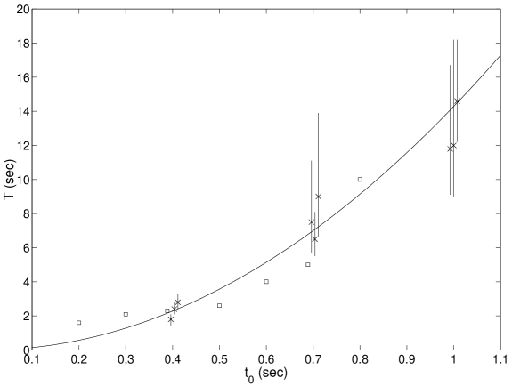
Figure 1: Experimentally obtained lifetimes $T$ (inverse switching rates) for the bistable perception of a non-continuously presented Necker cube. Crosses mark results from Kornmeier [14]: for each off-time $t_{0}$, $T$ (including standard errors) is plotted for three on-times of 0.05 sec, 0.1 sec, and 0.4 sec. Squares mark results from Orbach et al. [21] for an on-time of 0.3 sec (no errors indicated in [21]). The plotted curve shows $T$ as a function of off-times $t_{0}$ according to eq. 8 with $\Delta T=70$ msec.

4 Summary and conclusions

In the framework of a generalized, “weak” quantum theory, the quantum Zeno effect was applied to the bistable perception of ambiguous stimuli. In this application to a phenomenon of cognitive science, which obviously exceeds the domain of standard quantum physics, the quantum feature of measurement corresponds to the act of perception. The main result of this paper is the derivation and cognitive interpretation of three crucial time scales:

$\Delta T$:

the time between successive observations; as a lower bound for $\Delta T$ in cognitive operations, the so-called order threshold of $\approx 30$ msec is proposed.

$t_{0}$:

the oscillation period for the switching process between two non-stationary states under the unperturbed evolution of the system; $t_{0}$ will be increased to $T$ if measurements are carried out.

$T$:

the increased switching period for the case that measurements are carried out; cognitively this corresponds to the switching period of $\approx 3$ sec for bistable perception under continuous presentation of the stimulus.

The quantum Zeno model establishes a relation between these three time scales, yielding $t_{0}\gtrapprox 300$ msec for $\Delta T\gtrapprox 30$ msec and $T\approx 3$ sec under the condition of continuous stimulus presentation. Such a value of $t_{0}$ is often discussed as the approximate size of the time interval after which the processing of sensory inputs leads to a consciously available result, i.e. a mental representation of the stimulus.

Non-continuous presentation of the Necker cube provides the possibility to vary $t_{0}$ in an experimentally controlled manner in terms of off-times between stimulus presentation. Empirical results for $T$ as a function of $t_{0}$ support the relation between the three times scales with respect to their cognitive significance. However, further experimental material will be needed to firmly establish the cognitive relevance of the quantum Zeno time scales.

Another prediction of the cognitive quantum Zeno effect is the existence of superpositions $c_{1}\psi_{1}+c_{2}\psi_{2}$ of the individual well-defined perception states $\psi_{1}$ and $\psi_{2}$. It is presumably not easy to prepare and observe such superposition states. Nevertheless, they should appear at least as unstable, transitional states between $\psi_{1}$ and $\psi_{2}$. Elsewhere [1] such states were tentatively described as “acategoreal” states, indicating that they do not encode categoreal representations in the usual sense of cognitive science. In [15], a specific neural correlate of such states was for the first time reported in terms of an early (250 msec) component in event-related potentials.

An interesting option for the preparation of superposition states is the perception of paradoxical rather than ambiguous figures. In this case, the key idea is that both alternatives of perception operate as repellors rather than attractors, thus pushing the state of the system toward the unstable superposition in between them. So far, no experimental material is available concerning such a scenario.

References

- [1] H. Atmanspacher (1992): Categoreal and acategoreal representations of knowledge. Cognitive Systems 3, 259–288.
- [2] H. Atmanspacher, H. Römer and H. Walach (2002): Weak quantum theory: Complementarity and entanglement in physics and beyond. Foundations of Physics 32, 379–406.
- [3] H. Atmanspacher and T. Filk (2003): Discrimination and sequentialization of events in perception. In The Nature of Time, ed. by M. Saniga and R. Buccheri. Kluwer, Dordrecht, in press.
- [4] F. Beck and J. Eccles (1992): Quantum aspects of brain activity and the role of consciousness. Proceedings of the National Academy of Sciences of the USA 89, 11357–11361. See also F. Beck (2001): Quantum brain dynamics and consciousness. In The Physical Nature of Consciousness, ed. by P. van Loocke, Benjamins, Amsterdam, pp. 83–116.
- [5] K.T. Brown (1955): Rate of apparent change in a dynamic ambiguous figure as a function of observation time. American Journal of Psychology 68, 358–371.
- [6] F. Cajori (1915): The history of Zeno’s arguments on motion. American Mathematical Monthly 22, 1–6; 77–82; 109–115; 143–149; 179–186; 215–220; 253–258.
- [7] A. De Marco, P. Penengo, A. Trabucco, A. Borsellino, F. Carlini, M. Riani, and M.T. Tuccio (1977): Stochastic models and fluctuations in reversal time of ambiguous figures, Perception 6, 645–656.
- [8] E. Donchin, G. McCarthy, M. Kutas and W. Ritter (1983): Event-related brain potentials in the study of consciousness. In Consciousness and Self-Regulation, Vol. 3, ed. by R.J. Davidson, G.E. Schwartz and D. Shapiro, Plenum, New York, pp. 81–121.
- [9] R. Eckhorn and H.J. Reitböck (1989): Stimulus-specific synchronizations in cat visual cortex and their possible role in visual pattern recognition, in Synergetics of Cognition, ed. by H. Haken and M. Stadler, Springer, Berlin, pp. 99–111.
- [10] G.E. Gerstner and V.A. Fazio (1995): Evidence of a universal perceptual unit in mammals. Ethology 101, 89–100.
- [11] C.M. Gray and W. Singer (1989): Stimulus-specific neuronal oscillations in orientation columns of cat visual cortex. Proceedings of the National Academy of Sciences of the USA 86, 1698–1702.
- [12] D. Home and M.A.B. Whitaker (1997): A conceptual analysis of quantum Zeno; paradox, measurement and experiment. Annals of Physics 258, 237–285.
- [13] J. Kien and A. Kemp (1994): Is speech temporally segmented? Comparison with temporal segmentation in behavior. Brain and Language 46, 662–682.
- [14] J. Kornmeier (2002): Wahrnehmungswechsel bei mehrdeutigen Bildern – EEG-Messungen zum Zeitverlauf neuronaler Mechanismen. PhD thesis, University of Freiburg.
- [15] J. Kornmeier, M. Bach and H. Atmanspacher (2003): Correlates of perceptive instabilities in event-related potentials. International Journal of Bifurcations and Chaos, in press.
- [16] S. Kowal, D.C. O’Connell and E.J. Sabin (1975): Development of temporal patterning and vocal hesitations in spontaneous narratives. Journal of Psycholinguistic Research 4, 195–207.
- [17] P. Kruse and M. Stadler, eds. (1995): Ambiguity in Mind and Nature, Springer, Berlin.
- [18] D. Lehmann, H. Ozaki and I. Pal (1986): EEG alpha map series; brain micro-states by space-oriented adaptive segmentation. Electroencephalography and Clinical Neurophysiology 67, 271–288.
- [19] B. Misra and E.C.G. Sudarshan (1977): The Zeno’s paradox in quantum theory. Journal of Mathematical Physics 18, 756–763. See also K. Gustafson (2003): A Zeno story. Quantum Computers and Computing, in press.
- [20] L.A. Necker (1832): Observations on some remarkable phenomenon which occurs in viewing a figure of a crystal or geometrical solid. The London and Edinburgh Philosophy Magazine and Journal of Science 3, 329–337.
- [21] J. Orbach, E. Zucker and R. Olson (1966): Reversibility of the Necker cube VII. Reversal rate as a function of figure-on and figure-off durations. Perceptual and Motor Skills 22, 615–618.
- [22] R. Penrose (1994): Shadows of the Mind, Oxford University Press, Oxford. See also S.A. Hameroff and R. Penrose (1996): Conscious events as orchestrated spacetime selections. Journal of Consciousness Studies 3, 36–53.
- [23] L.B. Peterson and M.J. Peterson (1959): Short-term retention of individual items. Journal of Experimental Psychology 58, 193–198.
- [24] E. Plaum (1992): Bohrs quantentheoretische Naturbeschreibung und die Psychologie. Psychologie und Geschichte 3, 94–101.
- [25] E. Pöppel (1968): Oszillatorische Komponenten in Reaktionszeiten. Naturwissenschaften 55, 449–450.
- [26] E. Pöppel (1978): Time perception, in Handbook of Sensory Physiology Vol. 8, ed. by R. Held, H.W. Leibowitz and H.-L. Teubner, Springer, Berlin, pp. 713–729.
- [27] E. Pöppel (1997): A hierarchical model of temporal perception. Trends in Cognitive Sciences 1, 56–61. See also E. Pöppel (1997): The brain’s way to create “nowness”, in Time, Temporality, Now, ed. by H. Atmanspacher and E. Ruhnau, Springer, Berlin, pp. 107–120.
- [28] J. Radilova, E. Pöppel and J. Ilmberger (1990): Auditory reversal timing. Activitas Nervosa Superior 32, 137–138.
- [29] L.M. Ricciardi and H. Umezawa (1967): Brain and physics of many-body problems. Kybernetik 4, 44–48; G. Vitiello (2001): My Double Unveiled, Benjamins, Amsterdam, and references therein.
- [30] E. Ruhnau (1994): The now – a hidden window to dynamics, in Inside Versus Outside, ed. by H. Atmanspacher and G.J. Dalenoort, Springer, Berlin, pp. 291–308.
- [31] H.P. Stapp (1993): Mind, Matter, and Quantum Mechanics, Springer, Berlin.
- [32] H.P. Stapp (1999): Attention, intention, and will in quantum physics. Journal of Consciousness Studies 6, 143–164, particularly p. 159.
- [33] N. von Steinbüchel, M. Wittmann and E. Szelag (1999): Temporal constraints of perceiving, generating and integrating information: clinical indications. Restorative Neurology and Neuroscience 14, 167–182.
- [34] S. Sutton, M. Braren and J. Zubin (1965): Evoked potential correlates of stimulus uncertainty. Science 150, 1187–1188.
- [35] E. Szelag, N. von Steinbüchel, M. Reiser, E.G. de Langen and E. Pöppel (1996): Temporal constraints in processing nonverbal rhythmic patterns. Acta Neurobiologiae Experimentalis 56, 215–225.