The spectral and polarization characteristics of the nonspherically decaying radiation generated by polarization currents with superluminally rotating distribution patterns

Abstract

We present a theoretical study of the emission from a superluminal polarization current whose distribution pattern rotates (with an angular frequency $\omega$) and oscillates (with a frequency $\Omega$) at the same time, and which comprises both poloidal and toroidal components. This type of polarization current is found in recent practical machines designed to investigate superluminal emission. We find that the superluminal motion of the distribution pattern of the emitting current generates localized electromagnetic waves that do not decay spherically, i.e. that do not have an intensity diminishing like ${R_{P}}^{-2}$ with the distance $R_{P}$ from their source. The nonspherical decay of the focused wave packets that are emitted by the polarization currents does not contravene conservation of energy: the constructive interference of the constituent waves of such propagating caustics takes place within different solid angles on spheres of different radii ($R_{P}$) centred on the source. For a polarization current whose longitudinal distribution (over an azimuthal interval of length $2\pi$) consists of $m$ cycles of a sinusoidal wave train, the nonspherically decaying part of the emitted radiation contains the frequencies $\Omega\pm m\omega$; i.e. it contains only the frequencies involved in the creation and implementation of the source. This is in contrast to recent studies of the spherically decaying emission, which was shown to contain much higher frequencies. The polarization of the emitted radiation is found to be linear for most configurations of the source.

I Introduction

The electromagnetic field of a moving charged particle whose speed exceeds the speed of light in vacuo is the subject of several papers written by Sommerfeld in 1904 and 1905 [1], papers which were regarded to have been superseded by special relativity soon after their publication. One reason for abandoning further investigations of the work initiated by Sommerfeld, of course, was that any known particle that had a charge also had a rest mass and so was barred from moving faster than light by the requirements of special relativity. But there was an additional reason. Not even a massless particle can move faster than light in vacuo if it is charged; for if it does it would give rise to an infinitely strong electromagnetic field on the envelope of the wave fronts that emanate from it.

It was not until the appearance of the works of Ginzburg and his coworkers [2, 3, 4] that it was realized that, though no superluminal source of the electomagnetic field can be point-like, there are no physical principles disallowing faster-than-light sources that are extended. The coordinated motion of aggregates of subluminally moving charged particles of opposite sign can give rise to macroscopic polarization currents whose distribution patterns move superluminally. The electromagnetic field that is generated by such extended sources, on the other hand, may be built up by the superposition of the fields of their constituent volume elements, elements which individually act as the superluminally moving point sources considered by Sommerfeld [5, 6, 7, 8].

The purpose of the present paper is to examine the radiation field of a particular class of such volume-distributed sources: polarization currents whose distribution patterns have the time dependence of a travelling wave with a centripetally-accelerated superluminal motion. A motivation for this work is the recent design, construction and testing of experimental machines with this characteristic [9, 10, 11, 12, 13, 14].

The Green’s function for the problem we analyze is the familiar field of a uniformly rotating point source. This is the Liénard-Wiechert field that is encountered in the analysis of synchrotron radiation, except that here we do not restrict the speed of the source to the subluminal regime. This uniformly rotating point source is used as a basic volume element of the extended superluminal source, which is then treated in detail by superposing the Liénard-Wiechert fields of its constituent elements. We find that fundamentally new radiation processes come into play as a result of lifting the restriction to the subluminal regime, processes that have no counterparts in either the synchrotron or the Čerenkov effects.

This paper is organized as follows. Section II presents an introductory description of the principles behind our calculation of the emission. It includes a definition of frequencies (Table I) and polarization (Section IIE) of the source, which are later used to discuss the spectral characteristics and polarization of the emitted radiation. A detailed mathematical treatment is given in Section III, with the expression describing the nonspherically decaying component of the radiation [Eq. (57)] being derived and discussed in Section IIID. The nonspherically and spherically decaying components of the emission are compared in Section IV, and a summary is given in Section V.

II Preamble: formulation of the problem

The physical principles underlying the (mostly unexpected) consequences of the processes described in Section I are more transparent if we begin with a descriptive account of the building blocks of the (unavoidably lengthy) analysis that follows in Section III. Consider a localized charge $q$ (a charge with linear dimensions much smaller than the typical radiation wavelengths considered) which moves on a circle of radius $r$ with the constant angular velocity $\omega{\hat{\bf e}}_{z}$, i.e. whose path ${\bf x}(t)$ is given, in terms of the cylindrical polar coordinates $(r,\varphi,z)$, by

$$r={\rm const.},\quad z={\rm const.},\quad\varphi={\hat{\varphi}}+\omega t,$$

where ${\hat{\bf e}}_{z}$ is the basis vector associated with $z$, and ${\hat{\varphi}}$ the initial value of $\varphi$.

Having defined the path of what will constitute the basic element of our volume source, we shall use the remainder of this section to describe (A) the associated Liénard-Wiechert field, (B) the bifurcation surface which divides the volume of the source into parts with differeing influences on the field, (C) the Hadamard regularization technique for dealing with the singularities which are inevitably encountered in the fields from a superluminal source, (D) the focal regions in which the nonspherically decaying part of the emission is detectable and (E) the relationship between the polarization of the source and of the emission.

II.1 The Liénard-Wiechert fields

The Liénard-Wiechert electric and magnetic fields that arise from a superluminally moving charge $q$ with the trajectory described in Eq. (1) are given by

$${\bf E}({\bf x}_{P},t_{P})=q\sum_{t_{\rm ret}}\bigg{[}{(1-|{\dot{\bf x}}|^{2}/c^{2})({\hat{\bf n}}-{\dot{\bf x}}/c)\over|1-{\hat{\bf n}}\cdot{\dot{\bf x}}/c|^{3}R^{2}(t)}+{{\hat{\bf n}}{\bf\times}\{({\hat{\bf n}}-{\dot{\bf x}}/c){\bf\times}{\ddot{\bf x}}\}\over c^{2}|1-{\hat{\bf n}}\cdot{\dot{\bf x}}/c|^{3}R(t)}\bigg{]}$$

and ${\bf B}={\hat{\bf n}}{\bf\times}{\bf E}$. Here, the coordinates $({\bf x}_{P},t_{P})=(r_{P},\varphi_{P},z_{P},t_{P})$ mark the space-time of observation points, ${\dot{\bf x}}\equiv d{\bf x}/dt$, $c$ is the speed of light in vacuo, and $R$ and ${\hat{\bf n}}$ are the magnitude

$$R(t)=[(z_{P}-z)^{2}+{r_{P}}^{2}+r^{2}-2r_{P}r\cos(\varphi_{P}-{\hat{\varphi}}-\omega t)]^{1\over 2}$$

and the direction ${\hat{\bf n}}\equiv{\bf R}/R$ of the vector ${\bf R}(t)\equiv{\bf x}_{P}-{\bf x}(t)$. The summation extends over all values of the retarded time, i.e. all solutions $t_{\rm ret}<t_{P}$ of $h(t)\equiv t+R(t)/c=t_{P}$. This summation and the absolute-value signs in the factor $|1-{\hat{\bf n}}\cdot{\dot{\bf x}}/c|$, which stems from the evaluation of the Dirac delta function $\delta(t-t_{P}+R/c)$ in the classical expression for the retarded potential [Eq. (10) below], are omitted in most textbook derivations of Liénard-Wiechert fields because in the subluminal regime the retarded time is a single-valued function of the observation time and $1-{\hat{\bf n}}\cdot{\dot{\bf x}}/c$ is everywhere positive [15].

For a given point source $(r,{\hat{\varphi}},z)$ with $r\omega>c$ and various positions $(r_{P},\varphi_{P},z_{P})$ of the observation point, the dependence $t_{P}=h(t)$ of the reception time $t_{P}$ on the emission time $t$ can have one of the generic forms shown in Fig. 1.

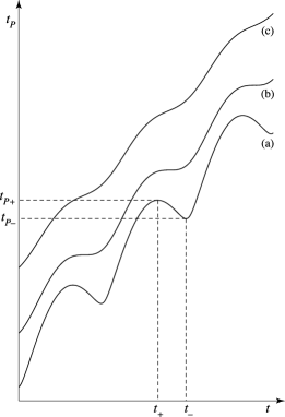
Figure 1: The relationship between the observation time $t_{P}$ and the emission time $t$ for an observation point that lies (a) inside or on, (b) on the cusp of, and (c) outside the envelope of the wave fronts or the bifurcation surface shown in Figs. 2 and 3. This relationship is given by $t_{P}=t+R(t)/c\equiv h(t;r,\varphi,z;r_{P},\varphi_{P},z_{P})$, an equation that applies to the envelope when the position $(r,\varphi,z)$ of the source point is fixed and to the bifurcation surface when the location $(r_{P},\varphi_{P},z_{P})$ of the observer is fixed. The maxima and minima of curve (a), at which $dR/dt=-c$, occur on the sheets $\phi_{+}$ and $\phi_{-}$ of the envelope or the bifurcation surface, respectively (Figs. 2 and 3). The inflection points of curve (b), at which $d^{2}R/dt^{2}=0$, occur on the cusp curve of the envelope or the bifurcation surface (Fig. 4).

As can be seen from curve (a) of this figure, there are values $t_{\pm}$ of the retarded time at which

$$1-{\hat{\bf n}}\cdot{\dot{\bf x}}/c={\dot{h}}(t)=1-r_{P}(r\omega/c)\sin(\varphi_{P}-\varphi+\omega t)/R(t)=0,$$

i.e. at which the source approaches the observer with the speed of light along the radiation direction ${\hat{\bf n}}$. The set of observation points at which the field receives contributions from the values $t_{\pm}$ of the retarded time are those located on the envelope of the wave fronts emanating from the moving source in question (Fig. 2). In the vicinity of the extrema of curve (a) in Fig. 1, the transcendental equation $t_{P}=h(t)$ for the retarded time reduces to

$$t_{P}=t_{P\pm}+\textstyle{1\over 2}{\ddot{h}}(t_{\pm})(t-t_{\pm})^{2}+\cdots,$$

where $t_{P\pm}\equiv h(t_{\pm})$ are the values of $t_{P}$ at which the waves emitted at $t=t_{\pm}$ arrive, and constructively interfere, at the envelope of the wave fronts (see Appendix C of [5]).

Were it to exist, a superluminally rotating point source would therefore generate an infinitely large field on the envelope of the wave fronts that would emanate from it: the Liénard-Wiechert fields diverge at the extrema of curve (a) in Fig. 1, where the factor $1-{\hat{\bf n}}\cdot{\dot{\bf x}}/c$ in the denominator of Eq. (2) vanishes. However, superluminal sources are necessarily extended and so it is only a superposition of the Liénard-Wiechert fields of their individual volume elements that is physically meaningful. The relevant quantity is the integral of the above field over the volume of $(r,{\hat{\varphi}},z)$ space that the moving localized source occupies in its rest frame.

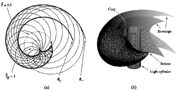
Figure 2: (a) Envelope of the spherical wave fronts emanating from a source point $S$ which moves with a constant angular velocity $\omega$ on a circle of radius $r=2.5c/\omega$ (${\hat{r}}\equiv r\omega/c=2.5$). The circles in broken lines designate the orbit of $S$ and the light cylinder $r_{P}=c/\omega$ (${\hat{r}}_{P}=1$). The curves to which the emitted wave fronts are tangent are the cross sections of the two sheets $\phi_{\pm}$ of the envelope with the plane of source’s orbit. (b) Three-dimensional view of the light cylinder and the envelope of wave fronts for the same source point $S$. The tube-like surface constituting the envelope is symmetric with respect to the plane of the orbit. The cusp along which the two sheets of this envelope meet touches, and is tangential to, the light cylinder at a point on the plane of the source’s orbit and spirals around the rotation axis out into the radiation zone. It approaches the cone $\theta_{P}=\arcsin(1/{\hat{r}})$ as $R_{P}$ tends to infinity ($R_{P}$, $\theta_{P}$ and $\varphi_{P}$ are the spherical coordinates of the observation point $P$).

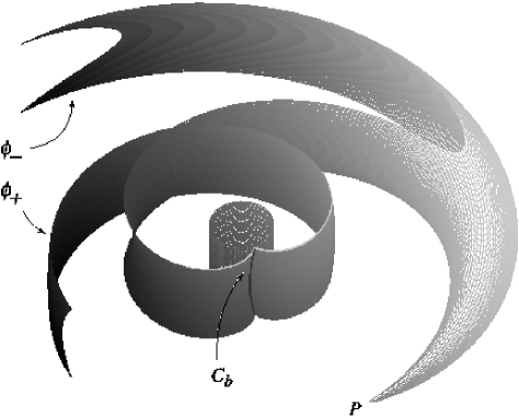
Figure 3: The bifurcation surface (i.e. the locus of source points that approach the observer along the radiation direction with the speed of light at the retarded time) associated with the observation point $P$ at the observation time $t_{P}$ (the motion of the source is clockwise). The cusp $C_{b}$, along which the two sheets of the bifurcation surface meet, touches and is tangent to the light cylinder (${\hat{r}}=1$) at a point on the plane passing through $P$ normal to the rotation axis. This cusp curve is the locus of source points which approach the observer not only with the speed of light ($dR/dt=-c$) but also with zero acceleration ($d^{2}R/dt^{2}=0$) along the radiation direction. For an observation point in the radiation zone, the spiralling surface that issues from $P$ undergoes a large number of turns, in which its two sheets intersect one another, before reaching the light cylinder.

II.2 The bifurcation surface of an observation point

Considering the field of a given point source, we have so far kept $(r,{\hat{\varphi}},z)$ fixed and have varied $(r_{P},{\hat{\varphi}}_{P},z_{P})$. If we now keep the observation point fixed and allow the coordinates $(r,{\hat{\varphi}},z)$ of the moving source point to sweep the rest-frame volume of an extended source, then the curves in Fig. 1 would represent the forms the relationship $t_{P}=h(t)$ assumes in different regions of the $(r,{\hat{\varphi}},z)$ space. For any given $(r_{P},{\hat{\varphi}}_{P},z_{P})$, there is a set of source elements of a volume source which approach the observer along the radiation direction ${\hat{\bf n}}$ with the speed of light at the retarded time, i.e. for which ${\dot{h}}=1-{\hat{\bf n}}\cdot{\dot{\bf x}}/c$ is zero. The locus of this set of source points in the $(r,{\hat{\varphi}},z)$ space is given by the intersection of the volume of the source with the two-sheeted surface $t_{P\pm}(r,{\hat{\varphi}},z;r_{P},\varphi_{P},z_{P})-t_{P}=0$, a surface that we shall refer to as the bifurcation surface of the observation point $P$ (Fig. 3). For all source points in the vicinity of this locus, the relationship between the retarded and the observation times has the form assumed by curve (a) of Fig. 1 in the neighbourhood of its extrema, i.e. is that given in Eq. (5).

The two sheets ($\pm$) of the bifurcation surface $t_{P\pm}(r,{\hat{\varphi}},z;r_{P},\varphi_{P},z_{P})-t_{P}=0$ meet tangentially along a cusp curve (Figs. 3 and 4). The source points on this cusp curve approach the observer not only with the wave speed (with $dR/dt=-c$) but also with zero acceleration ($d^{2}R/dt^{2}=0$) along the radiation direction. For such source points, the relationship between the retarded and the observation times has the form assumed by curve (b) of Fig. 1 in the neighbourhood of its inflection point.

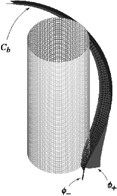
Figure 4: Close up of a segment of the cusp curve appearing in Fig. 3. The figure shows the section $0<{\hat{z}}-{\hat{z}}_{P}<5$ of the light cylinder (${\hat{r}}=1$) and the two sheets $\phi_{\pm}$ of the bifurcation surface (the locus of source points that approach the observer along the radiation direction with the speed of light at the retarded time) in the vicinity of its cusp curve $C_{b}$ (the locus of source points that approach the observer with the speed of light and zero acceleration) for an observer who is located at ${\hat{r}}_{P}=3$, ${\hat{\varphi}}_{P}=0$. The cusp curve $C_{b}$ is symmetrical with respect to the plane $z=z_{P}$ passing through the observation point $P$. The value ${G_{j}}^{\rm in}$ of the Green’s function $G_{j}$ inside the bifurcation surface diverges on the inner sides of the two sheets $\phi_{+}$ and $\phi_{-}$. The value ${G_{j}}^{\rm out}$ of $G_{j}$ outside the bifurcation surface undergoes a jump across the strip bordering on the cusp curve onto which these two sheets coalescence (in the limit ${\hat{R}}_{P}\gg 1$).

The retarded times from which the Liénard-Wichert field (2) receives singular contributions during any given period, therefore, are $t\simeq t_{+}\pm[2(t_{P}+-t_{P+})/{\ddot{h}}(t_{+})]^{1\over 2}$ for $t_{P}\,\mbox{{\raisebox{-1.72218pt}{$\stackrel{{\scriptstyle<}}{{{\scriptstyle\sim}}}$}}}\,t_{P+}$ and $t\simeq t_{-}\pm[2(t_{P}-t_{P-})/{\ddot{h}}(t_{-})]^{1\over 2}$ for $t_{P}\,\mbox{{\raisebox{-1.72218pt}{$\stackrel{{\scriptstyle>}}{{{\scriptstyle\sim}}}$}}}\,t_{P-}$ [see Eq. (5)]. Close to these retarded times, the factor $1-{\hat{\bf n}}\cdot{\dot{\bf x}}/c$ has the absolute value

$$|1-{\hat{\bf n}}\cdot{\dot{\bf x}}/c|=|{\dot{h}}(t)|\simeq[2{\ddot{h}}(t_{\pm})(t_{P}-t_{P\pm})]^{1\over 2}$$

according to Eq. (5). The functions $t_{P\pm}\equiv t_{\pm}+R(t_{\pm})/c$ in Eq. (6) depend linearly on the coordinate ${\hat{\varphi}}$ of the source point. This can be seen from Eq. (4) without solving for $t_{\pm}$: since $t$ in Eq. (4) appears in only the combination $\varphi_{P}-{\hat{\varphi}}-\omega t$, the solutions $t_{\pm}$ of this equation are given by expressions of the form $t_{\pm}=(\varphi_{\pm}-{\hat{\varphi}})/\omega$ in which $\varphi_{\pm}$ are functions of $(r,z)$ only. Given that the functions $R(t_{\pm})$ also depend on $t$ through $\varphi_{P}-{\hat{\varphi}}-\omega t$ and so are independent of ${\hat{\varphi}}$, it follows from $t_{P\pm}=t_{\pm}+R(t_{\pm})/c$ that $t_{P\pm}-t_{P}$ has the functional form $({\hat{\varphi}}_{\pm}-{\hat{\varphi}})/\omega$ in which ${\hat{\varphi}}_{\pm}$ depend on $r$ and $z$ only.

According to Eqs. (2) and (6), therefore, the Liénard-Wiechert fields diverge like $|{\hat{\varphi}}_{\pm}-{\hat{\varphi}}|^{-{3\over 2}}$ for those source elements close to the bifurcation surface ${\hat{\varphi}}={\hat{\varphi}}_{\pm}$ which approach the observer with the speed of light at the retarded time. This is a non-integrable singularity. To superpose the fields of the constituent volume elements of an extended source we need to integrate the expression that appears on the right-hand side of Eq. (2) over the volume of the $(r,{\hat{\varphi}},z)$ space occupied by that source. The multiple integral that needs to be evaluated here entails an integral with respect to ${\hat{\varphi}}$ whose integrand is proportional to $|{\hat{\varphi}}_{\pm}-{\hat{\varphi}}|^{-{3\over 2}}$ in the vicinity of ${\hat{\varphi}}={\hat{\varphi}}_{\pm}$ and so does not exist. Non-integrable singularities of this type commonly arise in the solutions of the wave equation over odd-dimensional space-times [16]; they can be handled by the following method from the theory of generalized functions, a method originally devised by Hadamard [16, 17, 18].

II.3 Hadamard’s regularization technique

Hadamard’s regularization technique is applicable to situations in which the superposition of the potentials of the volume elements of an extended source yields a differentiable function of the observer’s space-time coordinates, while the superposition of the fields of those same elements results in a divergent integral. This technique enables one to extract the physically relevant, finite value of the field of the extended source in question (which would follow from the differentiation of the potential owing to its entire volume) directly from the divergent integral that describes the superposition of the singular fields of its constituent elements. The calculation and subsequent differentiation of the potential owing to the entire source, a task which can hardly ever be performed analytically in physically realistic situations of this kind, is thus rendered unnecessary.

In the present case, the singularity of the Liénard-Wiechert potential is like $|1-{\hat{\bf n}}\cdot{\dot{\bf x}}/c|^{-1}\sim|{\hat{\varphi}}_{\pm}-{\hat{\varphi}}|^{-{1\over 2}}$ and so is integrable. The difficulty referred to above would not arise if we superposed the potentials, instead of the fields, of the consitituent volume elements of the source. We would know how to evaluate the required integral over $(r,{\hat{\varphi}},z)$, at least in principle, and the function of $({\bf x}_{P},t_{P})$ that we would thus obtain for the retarded potential of the entire source could then be differentiated to obtain a finite, singularity-free expression for the field. The non-integrable singularity we have encountered stems from interchanging the orders of integration and differentiation, from differentiating the Liénard-Wiechert potentials of the individual source elements (to obtain the fields) prior to integrating them over the source volume. Though feasible in principle, it is not of course practical to calculate the retarded potential of any physically viable extended source of the type we are considering explicitly. The regularization method we are about to describe is such, however, that the finite value it would assign to the divergent integral we have encountered exactly equals the value of the field which would follow from directly differentiating the retarded potential of the extended source [16, 17].

All the essential features of the mathematical problem that we face when atempting to integrate the Liénard-Wiechert field (2) with respect to the source coordinate ${\hat{\varphi}}$ are illustrated by the following simple example. Consider the function $f(x,a)=(a-x)^{-{1\over 2}}$. If we first evaluate the integral $I(a)=\int_{0}^{a}f(x,a)dx$ of this function with respect to $x$ and then differentiate the result ($I=2a^{1\over 2}$) with respect to $a$ we obtain the well-defined quantity $dI/da=a^{-{1\over 2}}$. But if we first differentiate $f(x,a)$ with respect to $a$ and then attempt to integrate the resulting function $\partial f/\partial a=-{1\over 2}(a-x)^{-{3\over 2}}$ over $x$, we obtain

$$J(a)\equiv\int_{0}^{a}dx\,\partial f/\partial a=-(a-x)^{-{1\over 2}}\big{|}_{x=a}+a^{-{1\over 2}},$$

a quantity which is divergent. The value which Hadamard’s regularization technique picks out as the finite part of the divergent integral $J(a)$ is $a^{-{1\over 2}}=dI/da$.

When applied to the more general form $\int_{0}^{a}dx\,F(x)(a-x)^{-{3\over 2}}$ of the above divergent integral, in which $F(x)$ is a regular function, Hadamard’s procedure consists of performing an integration by parts,

$$\int_{0}^{a}dx\,(a-x)^{-{3\over 2}}F(x)= 2(a-x)^{-{1\over 2}}F(x)\big{|}_{a}$$

$$-2a^{-{1\over 2}}F(0)-2\int_{0}^{a}dx\,(a-x)^{-{1\over 2}}\partial F(x)/\partial x,\quad (8)$$

and discarding the term which is divergent. The remaining finite part [consisting of the last two terms in Eq. (8)] is the value which Hadamard’s regularization assigns to this integral; it is the value one would obtain if one first evaluated $-2\int_{0}^{a}dx\,F(x)(a-x)^{-{1\over 2}}$ and then differentiated the result with respect to $a$.

The integral arising from the superposition of the Liénard-Wiechert fields of the constituent volume elements of a superluminally rotating charge distribution has an integrand which, in contrast to that of the integral in Eq. (8), is singular within the domain of integration (rather than on the boundary of this domain). Although such cases are seldom encountered in physics, their treatment using Hadamard’s regularization is well established in the theory of hyperbolic partial differential equations [16, 17]. [In the case of Čerenkov emission from an extended source, where there are no contributions from the source elements outside the bifurcation surface (the inverted Čerenkov cone issuing from the observation point), the corresponding singularity occurs on the boundary of the domain of integration.] Here, we have a divergent integral whose Hadamard finite part consists of two terms, an integrated term which turns out to decay like ${R_{P}}^{-{1\over 2}}$ with the distance $R_{P}$ from the source as $R_{P}$ tends to infinity, and an integral identical to the classical expression for the retarded field of a volume source [Eq. (14) of [19]] which decays spherically, like ${R_{P}}^{-1}$.

II.4 The nonsphericallly decaying part of the emission

The nonspherically decaying component of the radiation is detectable only within a limited region of space and during a limited interval of time: only when the cusps of the envelopes of wave fronts that emanate from the superluminally moving volume elements of the source propagate past the observer (see Fig. 2).

The radiated field entails, at any instant during this limited time interval, a set of wave envelopes (each associated with the wave fronts emanating from a specific member of a corresponding set of source elements) whose cusps pass through the position of the privileged observer in question. These caustics arise from those volume elements of the source which approach the observer, along the radiation direction, with the speed of light and zero acceleration at the retarded time (Figs. 3 and 4). It is the contribution toward the intensity of the field from the filamentary locus of such source elements that decays like ${R_{P}}^{-1}$ instead of ${R_{P}}^{-2}$.

The nonspherical decay of the field does not contravene conservation of energy. The focused wave packets that embody the nonspherically decaying pulses are constantly dispersed and reconstructed out of other waves, so that the constructive interference of their constituent waves takes place within different solid angles on spheres of different radii $R_{P}$ (see Appendix D of [5]). The integral of the flux of energy across a large sphere centred on the source is the same as the integral of the flux of energy across any other sphere that encloses the source. The strong fields that occur in focal regions are compensated by weaker fields elsewhere, so that the distribution of the flux of energy across such spheres is highly non-uniform and $R_{P}$-dependent.

II.5 Polarization of the source

This paper is specifically concerned with the spectral and polarization properties of the nonspherically decaying component of the radiation from a superluminal source. To assist in identifying the origins of the various polarization components in the emitted radiation, we base the analysis on a representative polarization current ${\bf j}=\partial{\bf P}/\partial t$ for which

$$P_{r,\varphi,z}(r,\varphi,z,t)=s_{r,\varphi,z}(r,z)\cos(m{\hat{\varphi}})\cos(\Omega t),\qquad-\pi<{\hat{\varphi}}\leq\pi,$$

with

$${\hat{\varphi}}\equiv\varphi-\omega t,$$

where $P_{r,\varphi,z}$ are the cylindrical components of the polarization (the electric dipole moment per unit volume), ${\bf s}(r,z)$ is an arbitrary vector that vanishes outside a finite region of the $(r,z)$ space and $m$ is a positive integer. Equation (9) generalizes the earlier calculation reported in [5], which was concerned with a rotating charge distribution, to a case in which the emitting polarization current flows in the $r$ and $z$ as well as in the $\varphi$ direction and has a distribution pattern that oscillates in addition to moving. This is similar to the polarization currents available within recently constructed machines built to study the physics of superluminal emission (see [9, 10, 11, 12, 13, 14] and Appendix A of [19]).

Symbol	Definition
$\omega$	Angular rotation frequency of the distibution pattern of the source
$\Omega$	The angular frequency with which the source oscillates (in addition to moving)
$f$	Frequency of the radiation generated by the source
$n=2\pi f/\omega$	The harmonic number associated with the radiation frequency
$m$	The number of cycles of the sinusoidal wave train representing the azimuthal
	dependence of the rotating source distribution [see Eq. (9)] around the
	circumference of a circle centred on, and normal to, the rotation axis
$|\Omega\pm m\omega|$	The two frequencies at which the nonspherically decaying component
	of the radiation from the source described in Eq. (9) is emitted. (The spectrum of the
	corresponding spherically decaying component of the radiation is limited to these two
	frequencies only if $\Omega/\omega$ is an integer.)

Table 1: Definition of the various frequencies and numbers used to describe the source and the emitted radiation

Note that the ranges of values of both $\varphi$ and $t$ in Eq. (9) are infinite, as in the case of a rotating point source, but the Lagrangian coordinate ${\hat{\varphi}}$, which labels each source element by its azimuthal position at $t=0$, lies in an interval of length $2\pi$ [19]. For a fixed value of $t$, the azimuthal dependence of the density (9) along each circle of radius $r$ within the source is the same as that of a sinusoidal wave train, with the wavelength $2\pi r/m$, whose $m$ cycles fit around the circumference of the circle smoothly. As time elapses, this wave train both propagates around each circle with the velocity $r\omega$ and oscillates in its amplitude with the frequency $\Omega$ (Table I). The vector ${\bf s}$ is here left arbitrary in order that we may investigate the polarization of the resulting radiation for all possible directions of the emitting current (Table II). Note that one can construct any distribution with a uniformly rotating pattern, $P_{r,\varphi,z}(r,{\hat{\varphi}},z)$, by the superposition over $m$ of terms of the form $s_{r,\varphi,z}(r,z,m)\cos(m{\hat{\varphi}})$.

III Detailed mathematical treatment of the problem

III.1 Integral representation of the Green’s function

In the absence of boundaries, the retarded potential $A^{\mu}$ arising from any localized distribution of charges and currents with a density $j^{\mu}$ is given by

$$A^{\mu}({\bf x}_{P},t_{P})=c^{-1}\int d^{3}x\,dt\,j^{\mu}({\bf x},t)\delta(t_{P}-t-R/c)/R,\quad\mu=0,\cdots,3$$

where $\delta$ is the Dirac delta function, $R$ stands for the magnitude of ${\bf R}\equiv{\bf x}_{P}-{\bf x}$, and $\mu=1,2,3$ designate the spatial components, ${\bf A}$ and ${\bf j}$, of $A^{\mu}$ and $j^{\mu}$ in a Cartesian coordinate system. For the purposes of calculating the electromagnetic fields

$${\bf E}=-{\bf\nabla}_{P}A^{0}-\partial{\bf A}/\partial(ct_{P})\qquad{\rm and}\qquad{\bf B}={\bf\nabla}_{P}{\bf\times A}$$

generated by the source in Eq. (9), the space-time of source points may be marked either with $({\bf x},t)=(r,\varphi,z,t)$ or with the coordinates $(r,{\hat{\varphi}},z,t)$ that naturally appear in the description of that rotating source. In fact, once ${\hat{\varphi}}$ is adopted as the coordinate that ranges over $(-\pi,\pi)$, the retarded position $\varphi$ of the rotating source point $(r,{\hat{\varphi}},z)$ as well as the retarded time $t$ could be used as the coordinate whose range is unlimited.

The electric current density ${\bf j}=\partial{\bf P}/\partial t$ that arises from the polarization distribution (9) is given, in terms of $\varphi$ and ${\hat{\varphi}}$, by the real part of

$${\bf j}=\textstyle{1\over 2}{\rm i}\omega\sum_{\mu=\mu_{\pm}}\mu\exp[-{\rm i}(\mu{\hat{\varphi}}-\Omega\varphi/\omega)]{\bf s},\quad-\pi<{\hat{\varphi}}\leq\pi,$$

where $\mu_{\pm}\equiv(\Omega/\omega)\pm m$. Changing the variables of integration in Eq. (10) from $({\bf x},t)=(r,\varphi,z,t)$ to $(r,\varphi,z,{\hat{\varphi}})$ and replacing ${\bf j}$ by the expression in Eq. (12), we obtain

$${\bf A}=\textstyle{1\over 2}{\rm i}(\omega/c)\sum_{\mu=\mu_{\pm}}\int_{V}dV\,\mu\exp(-{\rm i}\mu{\hat{\varphi}}){\bf s}\int_{\Delta\varphi}d\varphi\,\exp({\rm i}\Omega\varphi/\omega)\delta(g-\phi)/R(\varphi),$$

where $dV\equiv rdrd{\hat{\varphi}}dz$. Here $\phi$ stands for ${\hat{\varphi}}-{\hat{\varphi}}_{P}$ with ${\hat{\varphi}}_{P}\equiv\varphi_{P}-\omega t_{P}$, $R(\varphi)$ is

$$R(\varphi)=[(z_{P}-z)^{2}+{r_{P}}^{2}+r^{2}-2r_{P}r\cos(\varphi_{P}-\varphi)]^{1\over 2},$$

the function $g$ is defined by

$$g\equiv\varphi-\varphi_{P}+{\hat{R}}(\varphi),$$

with ${\hat{R}}\equiv R\omega/c$, $\Delta\varphi$ is the interval of azimuthal angle traversed by the source, and $V$ is the volume occupied by the source in the $(r,{\hat{\varphi}},z)$ space.

Terms of the order of $R^{-2}$ in ${\bf\nabla}_{P}{\bf\times A}$, which do not contribute toward the flux of energy at infinity, may be discarded, as usual [15], if we are concerned only with the radiation field. Since the problem we will be considering entails the formation of caustics, however, we need to treat the arguments of the delta function and its derivative in the resulting expression for ${\bf B}$ exactly. Approximating ${\bf\nabla}_{P}[R^{-1}\delta(t-t_{P}+R/c)]$ by $R^{-1}\delta^{\prime}(t-t_{P}+R/c){\bf\nabla}_{P}(R/c)$, i.e. discarding the term that arises from the differentiation of $R^{-1}$, we can therefore write the magnetic field of the radiation as

$${\bf B}\simeq \textstyle{1\over 2}{\rm i}(\omega/c)^{2}\sum_{\mu=\mu_{\pm}}\int_{V}dV\,\mu\exp(-{\rm i}\mu{\hat{\varphi}})\int_{\Delta\varphi}d\varphi\,\exp({\rm i}\Omega\varphi/\omega){\hat{\bf n}}\times{\bf s}$$

$$\times\delta^{\prime}(g-\phi)/R(\varphi), (16)$$

where ${\hat{\bf n}}={\bf R}(\varphi)/R(\varphi)$ and $\delta^{\prime}$ denotes the derivative of the delta function with respect to its argument.

To put the source density ${\bf s}=s_{r}{\hat{\bf e}}_{r}+s_{\varphi}{\hat{\bf e}}_{\varphi}+s_{z}{\hat{\bf e}}_{z}$ into a form suitable for inserting in Eq. (16), we need to express the $\varphi$-dependent base vectors $({\hat{\bf e}}_{r},{\hat{\bf e}}_{\varphi},{\hat{\bf e}}_{z})$ associated with the source point $(r,\varphi,z)$ in terms of the constant base vectors $({\hat{\bf e}}_{r_{P}},{\hat{\bf e}}_{\varphi_{P}},{\hat{\bf e}}_{z_{P}})$ at the observation point $(r_{P},\varphi_{P},z_{P})$:

$$\left[\matrix{{\hat{\bf e}}_{r}\cr{\hat{\bf e}}_{\varphi}\cr{\hat{\bf e}}_{z}\cr}\right]=\left[\matrix{\cos(\varphi-\varphi_{P})&\sin(\varphi-\varphi_{P})&0\cr-\sin(\varphi-\varphi_{P})&\cos(\varphi-\varphi_{P})&0\cr 0&0&1\cr}\right]\left[\matrix{{\hat{\bf e}}_{r_{P}}\cr{\hat{\bf e}}_{\varphi_{P}}\cr{\hat{\bf e}}_{z_{P}}\cr}\right].$$

Equation (17) together with the far-field value of ${\hat{\bf n}}$,

$$\lim_{R\to\infty}{\hat{\bf n}}=\sin\theta_{P}{\hat{\bf e}}_{r_{P}}+\cos\theta_{P}{\hat{\bf e}}_{z_{P}},\quad\theta_{P}\equiv\arctan(r_{P}/z_{P}),$$

yields the following expression for the source term in Eq. (16):

$${\hat{\bf n}}\times{\bf s}= [s_{r}\cos\theta_{P}\cos(\varphi-\varphi_{P})-s_{\varphi}\cos\theta_{P}\sin(\varphi-\varphi_{P})-s_{z}\sin\theta_{P}]{\hat{\bf e}}_{\parallel}$$

$$+[s_{\varphi}\cos(\varphi-\varphi_{P})+s_{r}\sin(\varphi-\varphi_{P})]{\hat{\bf e}}_{\perp}, (19)$$

where ${\hat{\bf e}}_{\parallel}\equiv{\hat{\bf e}}_{\varphi_{P}}$ (which is parallel to the plane of rotation) and ${\hat{\bf e}}_{\perp}\equiv{\hat{\bf n}}{\bf\times}{\hat{\bf e}}_{\parallel}$ comprise a pair of unit vectors normal to the radiation direction ${\hat{\bf n}}$.

Inserting Eq. (19) in Eq. (16), rewriting $\delta^{\prime}(g-\phi)$ as $-\partial\delta(g-\phi)/\partial{\hat{\varphi}}$ and making use of the fact that ${\hat{\bf n}}$, ${\bf s}$ and $\Delta\varphi$ are independent of ${\hat{\varphi}}$, we arrive at

$${\bf B}\simeq-\textstyle{1\over 2}{\rm i}(\omega/c)^{2}\sum_{\mu=\mu_{\pm}}\int_{V}dV\,\mu\exp(-{\rm i}\mu{\hat{\varphi}})\sum_{j=1}^{3}{\bf u}_{j}\partial G_{j}/\partial{\hat{\varphi}},$$

where

$${\bf u}_{1}\equiv s_{r}\cos\theta_{P}{\hat{\bf e}}_{\parallel}+s_{\varphi}{\hat{\bf e}}_{\perp},\quad{\bf u}_{2}\equiv-s_{\varphi}\cos\theta_{P}{\hat{\bf e}}_{\parallel}+s_{r}{\hat{\bf e}}_{\perp},\quad{\bf u}_{3}\equiv-s_{z}\sin\theta_{P}{\hat{\bf e}}_{\parallel},$$

and $G_{j}$ ($j=1,2,3$) are the functions resulting from the remaining integration with respect to $\varphi$:

$$\left[\matrix{G_{1}\cr G_{2}\cr G_{3}\cr}\right]=\int_{\Delta\varphi}d\varphi\,{\delta(g-\phi)\over R}\exp({\rm i}\Omega\varphi/\omega)\left[\matrix{\cos(\varphi-\varphi_{P})\cr\sin(\varphi-\varphi_{P})\cr 1\cr}\right].$$

The corresponding expression for the electric field is given by ${\bf E}\simeq{\hat{\bf n}}{\bf\times B}$, as in any other radiation problem.

The functions $G_{i}(r,{\hat{\varphi}},z;r_{P},{\hat{\varphi}}_{P},z_{P},\varphi_{P})$ here act as Green’s functions: they describe the fields of uniformly rotating point sources with fixed (Lagrangian) coordinates $(r,{\hat{\varphi}},z)$ whose strengths sinusoidally vary with time. In the special case in which $\Omega=0$, i.e. the strength of the source is constant, $G_{3}$ reduces to the Green’s function called $G_{0}$ in [5] and represents the Liénard-Wiechert potential of the point source described in Eq. (1). This may be seen by noting that the evaluation of the delta function in Eq. (22) yields

$$G_{3}\big{|}_{\Omega=0}=\sum_{\varphi=\varphi_{j}}{1\over R|\partial g/\partial\varphi|},$$

where $\varphi_{j}$ are the solutions of the transcendental equation $g(\varphi)=\phi$, solutions that are related to those of the equation $h(t)=t+R(t)/c=t_{P}$ for the retarded times via $\varphi={\hat{\varphi}}+\omega t$. The curves representing $g(\varphi)$ versus $\varphi$ have precisely the same forms as those appearing in Fig. 1.

Similarly, the vector $\partial(G_{2}\cos\theta_{P}{\hat{\bf e}}_{\perp}+G_{1}{\hat{\bf e}}_{\parallel})/\partial{\hat{\varphi}}$ is proportional to the Liénard-Wiechert field (2) when $\Omega$ is zero: the electric current associated with the rotating point source from which field (2) arises flows in the azimuthal direction and so corresponds to $s_{r}=s_{z}=0$. The singularity structures of $G_{i}$ are determined by the zeros of $\partial g/\partial\varphi$ or ${\dot{h}}$ [see Eq. (4)] and so are identical to the singularity structure already outlined in connection with $G_{0}$ in [5].

III.2 Asymptotic expansion of the Green’s function in the time domain

The retarded times at which the value of the Green’s function (23) [or that of the Liénard-Wiechert field (2)] receives divergent contributions from the point source $(r,{\hat{\varphi}},z)$ are given by the following solutions of $\partial g/\partial\varphi=0$ [or, equivalently, of Eq. (4)]:

$$\varphi_{\pm}=\varphi_{P}+2\pi-\arccos[(1\mp\Delta^{1\over 2})/({\hat{r}}{\hat{r}}_{P})],$$

with

$$\Delta\equiv({{\hat{r}}_{P}}^{2}-1)({\hat{r}}^{2}-1)-({\hat{z}}-{\hat{z}}_{P})^{2}$$

in which $({\hat{r}},{\hat{z}};{\hat{r}}_{P},{\hat{z}}_{P})$ stand for ($r\omega/c$, $z\omega/c$; $r_{P}\omega/c$, $z_{P}\omega/c$). Note that for a given observation point $(r_{P},\varphi_{P},z_{P},t_{P})$, the critical times $t_{\pm}=(\varphi_{\pm}-{\hat{\varphi}})/\omega$ exist (i.e. are real) only when the $(r,z)$ coordinates of the source point lie within the region $\Delta\geq 0$ of the $(r,z)$ space shown in Fig. 5.

Figure 5: The projection $\Delta=0$ of the cusp curve of the bifurcation surface onto $(r,z)$ space. The two sheets $\phi_{\pm}(r,z)$ of the bifurcation surface exist only for the values of $(r,z)$ in $\Delta\geq 0$. For a given $(r,z)$ in $\Delta\geq 0$, the source point $(r,{\hat{\varphi}},z)$ lies within the bifurcation surface for $\phi_{-}<{\hat{\varphi}}-{\hat{\varphi}}_{P}<\phi_{+}$ and outside this surface for other values of ${\hat{\varphi}}$. The source elements whose $(r,z)$ coordinates fall in $\Delta<0$ approach the observer with a speed $dR/dt<c$ at the retarded time and so make contributions toward the field that are no different from those made in the subluminal regime. The projection of the cusp curve of the envelope of wave fronts onto the $(r_{P},z_{P})$ space is also given by $\Delta=0$ and has the same shape: the function $\Delta$ is invariant under the transformation $(r,z;r_{P},z_{P})\to(r_{P},z_{P};r,z)$. That the cusp curve of the envelope approaches the cone $\theta_{P}=\arcsin(1/{\hat{r}})$ as $R_{P}$ tends to infinity can be seen here from the slopes of the asymptotes of the curve $\Delta=0$: these asymptotes, and so the segments ${\hat{z}}>{\hat{z}}_{P}$ and ${\hat{z}}<{\hat{z}}_{P}$ of the cusp curve, lie in the plane ${\hat{z}}={\hat{z}}_{P}$ for ${\hat{r}}=1+$ but open up and tend towards the vertical as ${\hat{r}}$ becomes increasingly greater than $1$.

The locus of source points in the $(r,{\hat{\varphi}},z)$ space for which $\partial g/\partial\varphi=0$ can be found by inserting $t_{\pm}=(\varphi_{\pm}-{\hat{\varphi}})/\omega$ in the equation $t_{P}-t-R/c=0$ which specifies the retarded times, or equivalently by inserting Eq. (24) in $g-\phi=0$ [see Eqs. (10), (13) and (15)]. The result is

$$\phi=\phi_{\pm}\equiv g(\varphi_{\pm})=2\pi-\arccos[(1\mp\Delta^{1\over 2})/({\hat{r}}{\hat{r}}_{P})]+{\hat{R}}_{\pm},$$

where

$${\hat{R}}_{\pm}\equiv{\hat{R}}(\varphi_{\pm})=[({\hat{z}}-{\hat{z}}_{P})^{2}+{\hat{r}}^{2}+{{\hat{r}}_{P}}^{2}-2(1\mp\Delta^{1\over 2})]^{1\over 2}.$$

The two sheets ($\pm$) of the tube-like spiralling surface ${\hat{\varphi}}={\hat{\varphi}}_{P}+\phi_{\pm}(r,z)$ meet tangentially and form a cusp where $\Delta=0$ (Figs. 3 and 4). This cusp curve on which $\partial^{2}g/\partial\varphi^{2}$ (and ${\ddot{h}}$) as well as $\partial g/\partial\varphi$ (and ${\dot{h}}$) are zero, constitutes the locus of source points which approach the observer, not only with the speed of light, but also with zero acceleration along the radiation direction. On it, the coalescence of two neighbouring stationary points of the phase function [curve (a) of Fig. 1] results in a point of inflection [curve (b) of Fig. 1] and so in a stronger singularity of the Green’s function.

For source points in the vicinity of this cusp curve, a unifrom asymptotic approximation to the value of the integral (22) defining the $G_{i}$ can be found by the method of Chester, Friedman and Ursell [20, 21]. Where it is analytic (i.e. for all ${\bf x}\neq{\bf x}_{P}$), the function $g(\varphi)$ in the argument of the delta function in Eq. (22) may be transformed into the following cubic function:

$$g(\varphi)=\textstyle{1\over 3}\nu^{3}-{c_{1}}^{2}\nu+c_{2},$$

where $\nu$ is a new variable of integration replacing $\varphi$, and the coefficients $c_{1}$ and $c_{2}$ are chosen such that the values of the two functions on opposite sides of Eq. (28) coincide at their extrema:

$$c_{1}\equiv(\textstyle{3\over 4})^{1\over 3}(\phi_{+}-\phi_{-})^{1\over 3},\quad c_{2}\equiv\textstyle{1\over 2}(\phi_{+}+\phi_{-}).$$

Insertion of Eq. (28) in Eq. (22) results in

$$G_{j}=\int_{\Delta\nu}d\nu\,f_{j}(\nu)\delta(\textstyle{1\over 3}\nu^{3}-{c_{1}}^{2}\nu+c_{2}-\phi)$$

where

$$\left[\matrix{f_{1}\cr f_{2}\cr f_{3}\cr}\right]=R^{-1}(d\varphi/d\nu)\exp({\rm i}\Omega\varphi/\omega)\left[\matrix{\cos(\varphi-\varphi_{P})\cr\sin(\varphi-\varphi_{P})\cr 1\cr}\right],$$

and $\Delta\nu$ is the image of $\Delta\varphi$ under transformation (28).

The leading term in the asymptotic expansion of the integral (30) for small $c_{1}$ can now be obtained [20, 22, 23, 24] by replacing its integrand $f_{j}$ with $p_{j}+q_{j}\nu$ and extending its range $\Delta\nu$ to $(-\infty,\infty)$:

$$G_{j}\sim\int_{-\infty}^{\infty}d\nu\,(p_{j}+q_{j}\nu)\delta(\textstyle{1\over 3}\nu^{3}-{c_{1}}^{2}\nu+c_{2}-\phi),$$

where

$$p_{j}=\textstyle{1\over 2}(f_{j}|_{\nu=c_{1}}+f_{j}|_{\nu=-c_{1}}),$$

$$q_{j}=\textstyle{1\over 2}{c_{1}}^{-1}(f_{j}|_{\nu=c_{1}}-f_{j}|_{\nu=-c_{1}}),$$

and the symbol $\sim$ denotes asymptotic approximation. (Note that the critical points $\varphi=\varphi_{\pm}$ transform into $\nu=\mp c_{1}$, respectively.) This integral has precisely the same form as that evaluated in Appendix A of [5].

It behaves differently inside ($\phi_{-}<\phi<\phi_{+}$) and outside ($\phi<\phi_{-},\,\phi>\phi_{+}$) the bifurcation surface so that

$$G_{j}=\cases{{G_{j}}^{\rm in}&$|\chi|<1$\cr{G_{j}}^{\rm out}&$|\chi|>1$,\cr}$$

with

$${G_{j}}^{\rm in}\sim 2{c_{1}}^{-2}(1-\chi^{2})^{-{1\over 2}}[p_{j}\cos(\textstyle{1\over 3}\arcsin\chi)-c_{1}q_{j}\sin(\textstyle{2\over 3}\arcsin\chi)],$$

$${G_{j}}^{\rm out}\sim{c_{1}}^{-2}(\chi^{2}-1)^{-{1\over 2}}[p_{j}\sinh(\textstyle{1\over 3}{\rm arccosh}|\chi|)+c_{1}q_{j}{\rm sgn}(\chi)\sinh(\textstyle{2\over 3}{\rm arccosh}|\chi|)],$$

and $\chi\equiv 3(\phi-c_{2})/(2{c_{1}}^{3})$ [cf. Eqs. (A16) and (A17) of [5]]. [The two-dimensional loci $\chi=\pm 1$ across which each $Gj$ changes form correspond, according to Eq. (29), to the two sheets $\phi_{\pm}$ of the bifurcation surface, respectively.] Explicit expressions for the coefficients $p_{j}(r,z)$ and $q_{j}(r,z)$ are given in Appendix A.

The above results show that as a source point $(r,{\hat{\varphi}},z)$ in the vicinity of the cusp curve approaches the bifurcation surface from inside, i.e. as $\chi\to 1-$ or $\chi\to-1+$, ${G_{j}}^{\rm in}$ and hence $G_{j}$ diverges. However, as a source point approaches one of the sheets of the bifurcation surface from outside, $G_{j}$ tends to a finite limit:

$${G_{j}}^{\rm out}\big{|}_{\phi=\phi_{\pm}}={G_{j}}^{\rm out}\big{|}_{\chi=\pm 1}\sim(p_{j}\pm 2c_{1}q_{j})/(3{c_{1}}^{2}),$$

for the numerator of ${G_{j}}^{\rm out}$ is also zero when $|\chi|=1$. The Green’s function $G_{j}$ is singular, in other words, only on the inner side of the bifurcation surface (see Fig. 6).

Figure 6: The $\chi$ dependence of the Green’s function $G_{1}$ in the far-field limit where $p_{1}=0$. The values of this function inside and outside the interval $-1<\chi<1$ represent ${G_{1}}^{\rm in}$ and ${G_{1}}^{\rm out}$, respectively: the space inside the bifurcation surface [the interval $\phi_{-}<\phi<\phi_{+}$ at a given $(r,z)$] is mapped into $|\chi|<1$ and that outside the bifurcation surface into $|\chi|>1$. The function ${G_{1}}^{\rm in}$ diverges on the inner sides, $\chi=1-$ and $\chi=-1+$, of the two sheets $\phi_{+}$ and $\phi_{-}$ of the bifurcation surface. The function ${G_{1}}^{\rm out}$ is discontinuous across a two-dimensional strip bordering on the cusp curve of the bifurcation surface: even at points close to this cusp curve where the separation $\phi_{+}-\phi_{-}$ of the two sheets of the bifurcation surface tends to zero (Figs. 3 and 4), the vanishingly small interval $\phi_{-}<\phi<\phi_{+}$ in $\phi$ is mapped into the finite interval $-1<\chi<1$ in $\chi$, so that the difference ${G_{1}}^{\rm out}|_{\chi=1+}-{G_{1}}^{\rm out}|_{\chi=-1-}$ between the values of the function ${G_{1}}^{\rm out}$ on opposite sides of the strip in question remains non-zero.

Moreover, like the diffraction field near a focal point [22], the Green’s function ${G_{j}}^{\rm out}$ undergoes a phase shift across the coalescent surfaces $\phi=\phi_{\pm}$ at the cusp curve (Fig. 4 and 6). The shift in the sign of the second term in Eq. (34c) results in a finite discontinuity in the value of ${G_{j}}^{\rm out}$ across the strip bordering on the cusp curve where the two sheets of the bifurcation surface are tangential: even in the limit $c_{1}\to 0$, where $\phi_{-}$ and $\phi_{+}$ are coincident, ${G_{j}}^{\rm out}|_{\phi=\phi_{+}}-{G_{i}}^{\rm out}|_{\phi=\phi_{-}}$ has the non-vanishing value ${4\over 3}q_{j}/c_{1}$. It is this discontinuity in the value of the Green’s function (the potential of a point source) across the cusp curve of the bifurcation surface that gives rise to nonspherically decaying boundary contributions to the field of a volume source. (Note that a discontinuity of this type, which resembles that of a step function, cannot be handled by means of an analysis in the frequency domain unless the contributions from an infinitely large number of Fourier components of the decomposed Green’s function are accurately superposed again when evaluating the field.)

III.3 Hadamard’s finite part of the integral representing the radiation field

The integral which represents the superposition of the contributions of the source elements in the vicinity of the cusp curve of the bifurcation surface to the value of the magnetic field, i.e. the integral resulting from the insertion of Eq. (34) in Eq. (20), is divergent: the derivative $\partial G_{j}/\partial{\hat{\varphi}}$ of the Green’s function has a singularity [$\sim(1-\chi^{2})^{-{3\over 2}}$] that is not integrable (with respect to $\chi$ or equivalently ${\hat{\varphi}}$).

Our task in this section is to extract the Hadamard finite part  [16, 17] of this divergent integral, the finite quantity that we would have obtained had we been able to evaluate the potential ${\bf A}({\bf x}_{P},t_{P})$ of the entire source explicitly prior to applying the operator ${\bf\nabla}_{P}\times$ to this potential.

The function $\partial G_{j}/\partial{\hat{\varphi}}$ appearing under the integral sign in Eq. (20) is given by different expressions in different regions of $(r,{\hat{\varphi}},z)$ space [see Eq. (34)]. For an observation point, the cusp curve of whose bifurcation surface intersects the source distribution, therefore, the domain of integration in Eq. (20) has to be divided into a part $V_{\rm in}$ that lies within and a part $V_{\rm out}$ that lies without the bifurcation surface before the integrand of the integral in this equation can be written out explicitly (Fig. 3). The Green’s function $G_{j}$ has no singularities in the region $\Delta<0$ of the $(r,z)$ space (Fig. 5), so that the contribution of the source elements in the part of $V_{\rm out}$ for which $\Delta<0$ are no different from the contributions of the source elements that lie in the subluminally moving portion of the source [see Eqs. (23)–(25)]. It would be sufficient to consider the contributions only of those source elements for which $\Delta\geq 0$. All source elements for which $\partial G_{j}/\partial{\hat{\varphi}}$ is singular are taken into account once the integration with respect to ${\hat{\varphi}}$ (at fixed values of $r$ and $z$ in $\Delta\geq 0$) is performed over the following two intervals: the interval $\phi_{-}<{\hat{\varphi}}-{\hat{\varphi}}_{P}<\phi_{+}$ in which $|\chi|<1$ and $G_{j}={G_{j}}^{\rm in}$, and the remaining part of $-\pi<{\hat{\varphi}}<\pi$ in which $|\chi|>1$ and $G_{j}={G_{j}}^{\rm out}$ (see Fig. 6).

Thus the magnetic field ${\bf B}_{\Delta\geq 0}$ that arises from the source elements in $\Delta\geq 0$ can be written, according to Eq. (20), as ${\bf B}^{\rm in}+{\bf B}^{\rm out}$ with

$${\bf B}^{\rm in,out}=-\textstyle{1\over 2}{\rm i}(\omega/c)^{2}\sum_{j=1}^{3}\int_{\Delta\geq 0}r\,dr\,dz\,{\bf u}_{j}{K_{j}}^{\rm in,out},$$

where

$${K_{j}}^{\rm in}\equiv\sum_{\mu=\mu_{\pm}}\int_{\phi_{-}}^{\phi_{+}}d\phi\,\mu\exp(-{\rm i}\mu{\hat{\varphi}})\partial{G_{j}}^{\rm in}/\partial{\hat{\varphi}},$$

and

$${K_{j}}^{\rm out}\equiv\sum_{\mu=\mu_{\pm}}\Big{(}\int_{-\pi-{\hat{\varphi}}_{P}}^{\phi_{-}}+\int_{\phi_{+}}^{\pi-{\hat{\varphi}}_{P}}\Big{)}d\phi\,\mu\exp(-{\rm i}\mu{\hat{\varphi}})\partial{G_{j}}^{\rm out}/\partial{\hat{\varphi}}.$$

(Recall that $dV\equiv rdrd{\hat{\varphi}}dz$ and $\phi\equiv{\hat{\varphi}}-{\hat{\varphi}}_{P}$.)

Once it is integrated by parts, the integral in Eq. (36b) in turn splits into two terms:

$${K_{j}}^{\rm in}=\sum_{\mu=\mu_{\pm}}\Big{\{}\Big{[}\mu\exp(-{\rm i}\mu{\hat{\varphi}}){G_{j}}^{\rm in}\Big{]}_{\phi_{-}}^{\phi_{+}}+{\rm i}\int_{\phi_{-}}^{\phi_{+}}d\phi\,{\mu}^{2}\exp(-{\rm i}\mu{\hat{\varphi}}){G_{j}}^{\rm in}\Big{\}},$$

of which the first (integrated) term is divergent [see Eq. (34) and Fig. 6]. Hadamard’s finite part of ${K_{j}}^{\rm in}$ and hence of ${\bf B}^{\rm in}$ (here designated by the prefix ${\cal F}$) is obtained by discarding this divergent contribution toward the value of ${K_{j}}^{\rm in}$ (see [16, 17, 18]):

$${\cal F}\big{\{}{K_{j}}^{\rm in}\big{\}}={\rm i}\sum_{\mu=\mu_{\pm}}\int_{\phi_{-}}^{\phi_{+}}d\phi\,{\mu}^{2}\exp(-{\rm i}\mu{\hat{\varphi}}){G_{j}}^{\rm in}.$$

Note that the singularity of the kernel of this integral, i.e. the singularity of ${G_{j}}^{\rm in}$, is like that of $|{\hat{\varphi}}_{\pm}-{\hat{\varphi}}|^{-{1\over 2}}$ and so is integrable.

The boundary contributions that result from the integration of the right-hand side of Eq. (36c) by parts are well-defined automatically:

$${K_{j}}^{\rm out}= \sum_{\mu=\mu_{\pm}}\Big{\{}\Big{[}\mu\exp(-{\rm i}\mu{\hat{\varphi}}){G_{j}}^{\rm out}\Big{]}_{\phi_{-}}^{\phi_{+}}$$

$$+{\rm i}\Big{(}\int_{-\pi-{\hat{\varphi}}_{P}}^{\phi_{-}}+\int_{\phi_{+}}^{\pi-{\hat{\varphi}}_{P}}\Big{)}d\phi{\mu}^{2}\exp(-{\rm i}\mu{\hat{\varphi}}){G_{j}}^{\rm out}\Big{\}}, (39)$$

for ${G_{j}}^{\rm out}$ tends to a finite limit as the bifurcation surface is approached from outside (Fig. 6) and ${G_{j}}^{\rm out}|_{\phi=\pi-{\hat{\varphi}}_{P}}$ equals ${G_{j}}^{\rm out}|_{\phi=-\pi-{\hat{\varphi}}_{P}}$ when $\phi_{\pm}\neq\pm\pi-{\hat{\varphi}}_{P}$. The integral representing ${K_{j}}^{\rm out}$, in other words, is finite by itself and needs no regularization.

If we now insert ${\cal F}\{{K_{j}}^{\rm in}\}$ and ${K_{j}}^{\rm out}$ from Eqs. (38) and (39) in Eq. (36a) and combine ${\bf B}^{\rm in}$ and ${\bf B}^{\rm out}$, we arrive at an expression for the Hadamard finite part of ${\bf B}_{\Delta\geq 0}$ which entails both a volume and a surface integral: ${\cal F}\{{\bf B}_{\Delta\geq 0}\}={\bf B}^{\rm s}+{\bf B}^{\rm ns}$. The volume integral

$${\bf B}^{\rm s}=\textstyle{1\over 2}(\omega/c)^{2}\sum_{\mu=\mu_{\pm}}\mu^{2}\int_{\Delta\geq 0}r\,dr\,dz\,\int_{-\pi}^{\pi}d{\hat{\varphi}}\,\exp(-{\rm i}\mu{\hat{\varphi}})\sum_{j=i}^{3}{\bf u}_{j}G_{j}$$

has the same form as the familiar integral representation of the field of a subluminal source [19] and decays spherically (like ${R_{P}}^{-1}$ for $R_{P}\to\infty$). The surface integral

$${\bf B}^{\rm ns}\equiv-\textstyle{1\over 2}{\rm i}(\omega/c)^{2}\sum_{j=1}^{3}\int_{\Delta\geq 0}r\,dr\,dz\,{\bf u}_{j}{K_{j}}^{\rm boundary}$$

stems from the boundary contribution

$${K_{j}}^{\rm boundary}\equiv\sum_{\mu=\mu_{\pm}}\Big{[}\mu\exp(-{\rm i}\mu{\hat{\varphi}}){G_{j}}^{\rm out}\Big{]}_{\phi_{-}}^{\phi_{+}}$$

in Eq. (39) and, as we shall see below, turns out to decay nonspherically (like ${R_{P}}^{-{1\over 2}}$ for $R_{P}\to\infty$).

Making use of Eq. (35) to rewrite ${G_{j}}^{\rm out}|_{\phi_{-}}^{\phi_{+}}$ in Eq. (42) explicitly, we obtain

$${K_{j}}^{\rm boundary}= \textstyle{2\over 3}\sum_{\mu=\mu_{\pm}}\mu\exp[-{\rm i}\mu({\hat{\varphi}}_{P}+c_{2})]\big{[}2{c_{1}}^{-1}q_{j}\cos(\textstyle{2\over 3}\mu{c_{1}}^{3})$$

$$-{\rm i}{c_{1}}^{-2}p_{j}\sin(\textstyle{2\over 3}\mu{c_{1}}^{3})\big{]}, (43)$$

where $c_{1}$ and $c_{2}$ are defined in Eq. (29). The asymptotic expansion of ${G_{j}}^{\rm out}$ in Eq. (34c) is for small $c_{1}$. To be consistent, therefore, we must likewise replace the above expression by the first term of its Taylor expansion in powers of $c_{1}$:

$${K_{j}}^{\rm boundary}=\textstyle{4\over 3}{c_{1}}^{-1}q_{j}\sum_{\mu=\mu_{\pm}}\mu\exp[-{\rm i}\mu({\hat{\varphi}}_{P}+\phi_{-})]+\cdots,$$

for the remainder of this series is by a factor of the order of ${c_{1}}^{2}$ smaller than the above retained term.

The value of $c_{1}$ close to the cusp curve of the bifurcation surface (where $\Delta=0$) is in turn given by

$$c_{1}=2^{-{1\over 3}}({\hat{r}}^{2}{{\hat{r}}_{P}}^{2}-1)^{-{1\over 2}}\Delta^{1\over 2}+O(\Delta).$$

This may be obtained by using Eq. (25) to express ${\hat{z}}$ everywhere in Eqs. (26) and (27) in terms of $\Delta$ and ${\hat{r}}$ and expanding the resulting expressions in powers of $\Delta^{1\over 2}$. When the observation point lies in the far zone, ${\hat{r}}$ on the cusp curve of the bifurcation surface has the value $\csc\theta_{P}$ [see Eq. (25)] and so $c_{1}$ assumes the value $2^{-{1\over 3}}{{\hat{R}}_{P}}^{-1}\Delta^{1\over 2}$. Moreover, according to Eqs. (A9) and (A10),

$$q_{j}\simeq 2^{2\over 3}(\omega/c){{\hat{R}}_{P}}^{-1}\exp[{\rm i}(\Omega/\omega)(\varphi_{P}+3\pi/2)]{\bar{q}}_{j}$$

with

$${\bar{q}}_{j}\equiv\big{(}1\quad-{\rm i}\Omega/\omega\quad{\rm i}\Omega/\omega\big{)}$$

for $\Delta\ll 1$ and ${\hat{R}}_{P}\gg 1$ (see Appendix A).

Equations (41), (44), (45) and (46) thus jointly yield

$${\bf B}^{\rm ns}\simeq -\textstyle{4\over 3}{\rm i}\exp[{\rm i}(\Omega/\omega)(\varphi_{P}+3\pi/2)]\sum_{\mu=\mu_{\pm}}\mu\exp(-{\rm i}\mu{\hat{\varphi}}_{P})$$

$$\times\sum_{j=1}^{3}{\bar{q}}_{j}\int_{\Delta\geq 0}{\hat{r}}\,d{\hat{r}}\,d{\hat{z}}\,\Delta^{-{1\over 2}}{\bf u}_{j}\exp(-{\rm i}\mu\phi_{-}). (47)$$

The integrand of the surface integral in Eq. (47) is still singular on the projection of the cusp curve of the bifurcation surface onto the $(r,z)$ space (Fig. 5) but this singularity is integrable.

III.4 Amplitude, frequencies and polarization of the nonspherically decaying radiation outside the plane of source’s orbit

The leading term in the asymptotic expansion of the integral in Eq. (47) for high $\mu_{\pm}$ (i.e. for the regime in which the wavelengths of oscillations of the source are much shorter than the length scale $c/\omega$ of its orbit) may be obtained by the method of stationary phase provided that $\theta_{P}\neq\pi/2$.

Both derivatives, $\partial\phi_{-}/\partial{\hat{r}}$ and $\partial\phi_{-}/\partial{\hat{z}}$, of the function that appears in the phase of the rapidly oscillating exponential in Eq. (47) vanish at the point ${\hat{r}}=1$, ${\hat{z}}={\hat{z}}_{P}$, where the cusp curve of the bifurcation surface touches, and is tangential to, the light cylinder (see Figs. 3 and 4). However, $\partial^{2}\phi_{-}/\partial{\hat{r}}^{2}$ diverges at this point, so that neither the phase nor the amplitude of the integrand of the integral in Eq. (47) are analytic at ${\hat{r}}=1,{\hat{z}}={\hat{z}}_{P}$. Only for an observer who is located outside the plane of rotation, i.e. whose coordinate $z_{P}$ does not match the coordinate $z$ of any source element, is the function $\phi_{-}$ analytic throughout the domain of integration. To take advantage of the simplifications offered by the analyticity of $\phi_{-}$ as a function of ${\hat{r}}$, we proceed under the assumption that $\theta_{P}\neq\pi/2$.

Since $\phi_{-}\equiv g(\varphi_{-})$ and $\partial g/\partial\varphi=\partial g/\partial r=0$ along the curve

$$C:\quad {\hat{r}}={\hat{r}}_{C}({\hat{z}})\equiv\{\textstyle{1\over 2}({{\hat{r}}_{P}}^{2}+1)-[\textstyle{1\over 4}({{\hat{r}}_{P}}^{2}-1)^{2}-({\hat{z}}-{\hat{z}}_{P})^{2}]^{1\over 2}\}^{1\over 2},$$

$$\varphi=\varphi_{C}({\hat{z}})\equiv\varphi_{P}+2\pi-\arccos({\hat{r}}_{C}/{\hat{r}}_{P}) (48)$$

[Eqs. (15) and (26)], $\phi_{-}$ is stationary as a function of ${\hat{r}}$, i.e.  $\partial\phi_{-}/\partial{\hat{r}}=0$, on the projection ${\hat{r}}_{C}({\hat{z}})$ of $C$ onto the $(r,z)$ plane (see also [19]). In the far-field limit, where the terms $({\hat{z}}-{\hat{z}}_{P})^{2}/({{\hat{r}}_{P}}^{2}-1)^{2}$ and ${\hat{r}}_{C}/{\hat{r}}_{P}$ in Eq. (48) are much smaller than unity, curve $C$ coincides with the locus

$$C_{b}:\quad {\hat{r}}=[1+({\hat{z}}-{\hat{z}}_{P})^{2}/({{\hat{r}}_{P}}^{2}-1)]^{1\over 2},$$

$$\varphi=\varphi_{P}+2\pi-\arccos[1/({\hat{r}}{\hat{r}}_{P})], (49)$$

of source points which approach the observer along the radiation direction with the wave speed and zero acceleration at the retarded time, i.e. coincides with the cusp curve of the bifurcation surface (Figs. 3 and 4).

It can be seen from the far-field limit of Eq. (49) that the cusp curve $C_{b}$ would intersect the source distribution if $\theta_{P}$ lies in the interval $|\theta_{P}-{\pi\over 2}|\leq\arccos\,(1/{{\hat{r}}_{>}})$, where ${\hat{r}}_{>}\equiv r_{>}\omega/c$ and $r_{>}$ is the radial coordinate of the outer boundary of the source [5]. Hence, the range of values of $\theta_{P}$ for which the stationary points of $\phi_{-}$ fall within the source distribution would be as wide as $(0,\pi)$ if the extent $r_{>}-c/\omega$ of the superlumially moving part of the source is comparable to the radius $c/\omega$ of the light cylinder (see Fig. 5).

The dominant terms in the Taylor expansion of $\phi_{-}$ about a point $({\hat{r}}_{C},\varphi_{C},{\hat{z}})$ on curve $C$ (with an arbitrary coordinate ${\hat{z}}\neq{\hat{z}}_{P}$) are

$$\phi_{-}=\phi_{C}-[\textstyle{1\over 2}({{\hat{r}}_{P}}^{2}-1)({{\hat{r}}_{C}}^{2}-1)^{-1}-1]{{\hat{R}}_{C}}^{-1}({\hat{r}}-{\hat{r}}_{C})^{2}+\cdots,$$

in which we have denoted the values of $\phi$ and ${\hat{R}}$ on $C$ by $\phi_{C}\equiv{\hat{R}}_{C}+\varphi_{C}-\varphi_{P}$ and

$${\hat{R}}_{C}\equiv[({\hat{z}}_{P}-{\hat{z}})^{2}+{{\hat{r}}_{P}}^{2}-{{\hat{r}}_{C}}^{2}]^{1\over 2},$$

respectively. Moreover, $\Delta^{1\over 2}$ has the finite value ${{\hat{r}}_{C}}^{2}-1$ on $C$ [Eqs. (25) and (48)].

We are now in a position to evaluate the leading term in the asymptotic expansion of the ${\hat{r}}$ integral in Eq. (47) by applying the principle of stationary phase [23, 24]: by replacing the phase of the rapidly oscillating exponential that appears in this integral with its Taylor expansion (50) and approximating the amplitude of the integrand with its value along $C$. The resulting integral, at a given value of ${\hat{z}}$, is

$$\int_{\Delta\geq 0}{\hat{r}}\,d{\hat{r}}\, \Delta^{-{1\over 2}}{\bf u}_{j}\exp(-{\rm i}\mu\phi_{-})\sim\exp(-{\rm i}\mu\phi_{C}){\hat{r}}_{C}({{\hat{r}}_{C}}^{2}-1)^{-1}{\bf u}_{j}\big{|}_{C}$$

$$\times\int_{0}^{{\hat{r}}_{>}-{\hat{r}}_{C}}d\eta\,\exp\{{\rm i}\mu[\textstyle{1\over 2}({{\hat{r}}_{P}}^{2}-1)({{\hat{r}}_{C}}^{2}-1)^{-1}-1]{{\hat{R}}_{C}}^{-1}\eta^{2}\}, (52)$$

in which ${\hat{r}}_{C}$, $\phi_{C}$ and ${\hat{R}}_{C}$ have their far-field values

$${\hat{r}}_{C}\simeq\csc\theta_{P},\quad\phi_{C}\simeq 3\pi/2+{\hat{R}}_{C},\quad{\hat{R}}_{C}\simeq{\hat{R}}_{P}-{\hat{z}}\cos\theta_{P},$$

and $\eta\equiv{\hat{r}}-{\hat{r}}_{C}$ [see Eqs. (48) and (51)]. This integral entails an integrand whose phase is large on account of both $\mu_{\pm}\gg 1$ and ${\hat{R}}_{P}\gg 1$. It can be cast into the form of, and evaluated as, a Fresnel integral with a large argument to arrive at

$$\int_{\Delta\geq 0}{\hat{r}}\,d{\hat{r}}\,\Delta^{-{1\over 2}}{\bf u}_{j}\exp(-{\rm i}\mu\phi_{-})\sim (\pi/2)^{1\over 2}{{\hat{R}}_{P}}^{-{1\over 2}}|\sin\theta_{P}\cos\theta_{P}|^{-1}|\mu|^{-{1\over 2}}$$

$$\times\exp[-{\rm i}(\mu\phi_{C}-\textstyle{\pi\over 4}{\rm sgn}\,\mu)]{\bf u}_{j}\big{|}_{C} (54)$$

when $\theta_{P}\neq\pi/2$. Note that the values ${\bf u}_{j}|_{C}$ of ${\bf u}_{j}$ along the curve $C$ are functions of $z$ and that this curve becomes parallel to the $z$ axis as $R_{P}$ tends to infinity (Figs. 4 and 5).

Once the surface integration in Eq. (47) is expressed in terms of a double integral, this result may be used to obtain

$${\bf B}^{\rm ns}\sim -\textstyle{4\over 3}{\rm i}(2\pi)^{1\over 2}{{\hat{R}}_{P}}^{-{1\over 2}}|\sin 2\theta_{P}|^{-1}\exp({\rm i}\Omega\varphi_{C}/\omega)\sum_{\mu=\mu_{\pm}}|\mu|^{1\over 2}{\rm sgn}(\mu)\exp({\rm i}\textstyle{\pi\over 4}{\rm sgn}\,\mu)$$

$$\times\exp[-{\rm i}\mu({\hat{R}}_{P}-\omega t_{P}+\varphi_{C})]\sum_{j=1}^{3}{\bar{q}}_{j}\int_{-\infty}^{\infty}d{\hat{z}}\,{\bf u}_{j}\big{|}_{C}\exp({\rm i}\mu{\hat{z}}\cos\theta_{P}), (55)$$

in which $\varphi_{C}\equiv\varphi_{P}+3\pi/2$. The remaining ${\hat{z}}$ integration in this expression amounts to a Fourier decomposition of the source densities $s_{r,\varphi,z}|_{C}$.

Insertion of Eqs. (21) and (46b) in Eq. (55) and the introduction of the Fourier transforms

$${\bar{s}}_{r,\varphi,z}\equiv\int_{-\infty}^{\infty}d{\hat{z}}\,s_{r,\varphi,z}\big{|}_{C}\exp({\rm i}\mu{\hat{z}}\cos\theta_{P}).$$

result in

$${\bf E}^{\rm ns}\sim \textstyle{4\over 3}(2\pi)^{1\over 2}{{\hat{R}}_{P}}^{-{1\over 2}}|\sin 2\theta_{P}|^{-1}\exp({\rm i}\Omega\varphi_{C}/\omega)\sum_{\mu=\mu_{\pm}}|\mu|^{1\over 2}{\rm sgn}(\mu)\exp({\rm i}\textstyle{\pi\over 4}{\rm sgn}\,\mu)$$

$$\times\exp[-{\rm i}\mu({\hat{R}}_{P}-\omega t_{P}+\varphi_{C})]\big{\{}({\rm i}{\bar{s}}_{\varphi}+\Omega{\bar{s}}_{r}/\omega){\hat{\bf e}}_{\parallel}$$

$$-[({\rm i}{\bar{s}}_{r}-\Omega{\bar{s}}_{\varphi}/\omega)\cos\theta_{P}+\Omega{\bar{s}}_{z}\sin\theta_{P}/\omega]{\hat{\bf e}}_{\perp}\big{\}} (57)$$

for the electric field (${\bf E}^{\rm ns}\sim{\hat{\bf n}}{\bf\times}{\bf B}^{\rm ns}$) of the nonspherically decaying part of the radiation. This expression is valid, of course, only for an observation point, outside the plane of rotation, the cusp curve of whose bifurcation surface intersects the source distribution, i.e. for $0<|\theta_{P}-{\pi\over 2}|\leq\arccos\,(1/{{\hat{r}}_{>}})$.

Thus the spectrum of the nonspherically decaying part of the radiation only contains the frequencies $\mu_{\pm}\omega=\Omega\pm m\omega$, i.e. the frequencies that enter the creation or practical implementation of the source described in Eq. (9). This contrasts with the spectrum of the spherically spreading part of the radiation which extends to frequencies of the order of $\Omega^{3}/\omega^{2}$ when $\Omega/\omega\gg 1$ (cf.  [19]). The intensity of the radiation at the frequency $\Omega+m\omega$ is the same as its intensity at $\Omega-m\omega$ when either $\Omega/\omega\gg m$ or $\Omega/\omega\ll m$. The radiation at one of these frequencies would have a much lower intensity, on the other hand, if $\Omega$ and $m\omega$ are comparable in magnitude.

Equation (57) shows, moreover, that the nonspherically decaying component of the radiation is linearly polarized both for $\Omega/\omega\ll 1$ and for $\Omega/\omega\gg 1$ when one of the cylindrical components of ${\bar{\bf s}}$ is appreciably larger than the others. In the case of an ${\bf s}$ which lies in the azimuthal direction, the radiation is polarized parallel to the plane of rotation for $\Omega/\omega\ll 1$ and normal to that direction (and phase shifted by $\pi/2$) for $\Omega/\omega\gg 1$. The plane of polarization of the radiation coincides with the plane passing through the observer and the rotation axis if ${\bf s}$ lies parallel to the rotation axis. For this radiation to be elliptically polarized, on the other hand, ${\bar{\bf s}}$ needs to have two cylindrical components that are comparable in magnitude and $\Omega/\omega$ has to be of the order of unity (Table 2).

	$\frac{\Omega}{\omega}\gg 1$	$\frac{\Omega}{\omega}\sim 1$	$\frac{\Omega}{\omega}\ll 1$
$s_{r}\neq 0,s_{\varphi}=s_{z}=0$	linear, ${\hat{\bf e}}_{\parallel}$, phase$=0$	elliptic	linear, ${\hat{\bf e}}_{\perp}$, phase$=-\frac{\pi}{2}$
$s_{\varphi}\neq 0,s_{r}=s_{z}=0$	linear, ${\hat{\bf e}}_{\perp}$, phase$=0$	elliptic	linear, ${\hat{\bf e}}_{\parallel}$, phase$=+\frac{\pi}{2}$
$s_{z}\neq 0,s_{r}=s_{\varphi}=0$	linear, ${\hat{\bf e}}_{\perp}$, phase$=\pi$	linear, ${\hat{\bf e}}_{\perp}$, phase$=\pi$	linear, ${\hat{\bf e}}_{\perp}$, phase$=\pi$

Table 2: The state of polarization of the nonspherically decaying component of the emitted radiation for different ranges of $\Omega/\omega$ and different orientations of the emitting polarization current

IV Discussion: comparison of the nonspherically and spherically decaying components of the radiation

The radiation field that arises from the superluminal portion ($r>c/\omega$) of the volume source described in Eq. (9) consists, as shown in the preceding section, of two components: a nonspherically decaying component whose intensity diminishes like ${R_{P}}^{-1}$ with the distance $R_{P}$ from the source and a spherically spreading component, one whose intensity has the conventional dependence ${R_{P}}^{-2}$ on $R_{P}$. The former is described by Eq. (57) and the latter, which follows from Eq. (40), was earlier calculated in [19]. The nonspherically decaying part of the radiation ${\bf E}^{\rm ns}$ is only emitted at the two frequencies $\mu_{\pm}\omega$, whereas the spherically decaying part ${\bf E}^{\rm s}$ has a discrete spectrum, comprising multiples $n\omega$ of the rotation frequency, which extends as far as $n\sim(\Omega/\omega)^{3}$ when $\Omega/\omega$ ($\gg 1$) is different from an integer (see Table I).

As in the case of any other linear system, the present emission process generates an output only at those frequencies which are carried both by its input (the source) and its response (Green’s) function. The agent responsible for the generation of a broadband radiation from the source described in Eq. (9), whose creation or practical implementation only entails the two frequencies $\mu_{\pm}\omega$, is acceleration: a remarkable effect of centripetal acceleration is to enrich the spectral content of a rotating volume source, for which $\Omega/\omega$ is different from an integer, by effectively endowing the distribution of its density with space-time discontinuities. (For a detailed discussion of this point, see [19].)

The electric field of the spherically spreading part of the radiation for incommensurate values of $\Omega$ and $\omega$ is given by the real part of

$${\bf E}^{\rm s}={{\tilde{\bf E}}^{\rm s}}_{0}+2\sum_{n=1}^{\infty}{{\tilde{\bf E}}^{\rm s}}_{n}\exp(-{\rm i}n{\hat{\varphi}}_{P}),$$

in which the Fourier component ${{\tilde{\bf E}}^{\rm s}}_{n}$ of this field at the frequency $n\omega$ has the following value beyond the Fresnel zone:

$${{\tilde{\bf E}}^{\rm s}}_{n}\sim \textstyle{1\over 2}{{\hat{r}}_{P}}^{-1}\exp\{-{\rm i}[n({\hat{R}}_{P}+\textstyle{3\over 2}\pi)-(\Omega/\omega)(\varphi_{P}+\textstyle{3\over 2}\pi)]\}({\hat{r}}_{>}-{\hat{r}}_{<})Q_{\hat{\varphi}}{\bar{\bf Q}}_{z}$$

$$+\{m\to-m,\Omega\to-\Omega\}, (59)$$

with

$$Q_{\hat{\varphi}}=-\sum_{\mu=\mu_{\pm}}\mu^{2}\sin[\pi(n-\mu)]/(n-\mu),$$

and

$${\bar{\bf Q}}_{z}\equiv \big{[}{\bar{s}}_{r}{\bf J}_{n-\Omega/\omega}(n)+{\rm i}{\bar{s}}_{\varphi}{{\bf J}^{\prime}}_{n-\Omega/\omega}(n)\big{]}{\hat{\bf e}}_{\parallel}+\big{[}({\bar{s}}_{\varphi}\cos\theta_{P}$$

$$-{\bar{s}}_{z}\sin\theta_{P}){\bf J}_{n-\Omega/\omega}(n)-{\rm i}{\bar{s}}_{r}\cos\theta_{P}{{\bf J}^{\prime}}_{n-\Omega/\omega}(n)\big{]}{\hat{\bf e}}_{\perp} (61)$$

[cf. Eq. (66) of [19]]. Here, ${\hat{r}}_{<}<1$ and ${\hat{r}}_{>}>1$ denote the lower and upper limits of the radial interval in which the source densities $s_{r,\varphi,z}$ are non-zero, the symbol $\{m\to-m,\Omega\to-\Omega\}$ designates a term like the one preceding it in which $m$ and $\Omega$ are everywhere replaced by $-m$ and $-\Omega$, respectively, and ${\bf J}_{n-\Omega/\omega}(n)$ and ${{\bf J}^{\prime}}_{n-\Omega/\omega}(n)$ are the Anger function [25] and the derivative of the Anger function with respect to its argument.

To compare the amplitudes of ${\bf E}^{\rm ns}$ and ${\bf E}^{\rm s}$ at a frequency with which both these components are emitted, let us consider a case in which $\Omega/\omega$ equals an integer, so that the spherically decaying part of the radiation is also emitted only at the frequencies $\mu_{\pm}\omega$. In this case, the quantity $Q_{\hat{\varphi}}$ in Eq. (60) is non-zero only if $n$ equals $\mu_{+}$ or $\mu_{-}$, and $Q_{\hat{\varphi}}|_{n=\mu_{\pm}}=-\pi{\mu_{\pm}}^{2}$.

At the higher of the two frequencies, i.e. at $\mu_{+}\omega=\Omega+m\omega$, the amplitude of ${\bf E}^{\rm ns}$ has the value

$$|{{\bf E}^{\rm ns}}_{\mu_{+}}|\sim \textstyle{4\over 3}(2\pi)^{1\over 2}{{\hat{R}}_{P}}^{-{1\over 2}}|\sin 2\theta_{P}|^{-1}{\mu_{+}}^{1\over 2}\big{|}({\rm i}{\bar{s}}_{\varphi}+\Omega{\bar{s}}_{r}/\omega){\hat{\bf e}}_{\parallel}$$

$$-[({\rm i}{\bar{s}}_{r}-\Omega{\bar{s}}_{\varphi}/\omega)\cos\theta_{P}+\Omega{\bar{s}}_{z}\sin\theta_{P}/\omega]{\hat{\bf e}}_{\perp}\big{|} (62)$$

according to Eq. (57). This should be compared with the following amplitude implied by Eqs. (58)–(61):

$$|{{\tilde{\bf E}}^{\rm s}}_{\mu_{+}}|\sim \textstyle{1\over 2}\pi{{\hat{r}}_{P}}^{-1}({\hat{r}}_{>}-{\hat{r}}_{<}){\mu_{+}}^{2}\big{|}[{\bar{s}}_{r}J_{m}(\mu_{+})+{\rm i}{\bar{s}}_{\varphi}{J^{\prime}}_{m}(\mu_{+})]{\hat{\bf e}}_{\parallel}$$

$$+[({\bar{s}}_{\varphi}\cos\theta_{P}-{\bar{s}}_{z}\sin\theta_{P})J_{m}(\mu_{+})-{\rm i}{\bar{s}}_{r}\cos\theta_{P}{J^{\prime}}_{m}(\mu_{+})]{\hat{\bf e}}_{\perp}\big{|} (63)$$

since the Anger functions ${\bf J}_{n-\Omega/\omega}(n)$ and ${{\bf J}^{\prime}}_{n-\Omega/\omega}(n)$ in Eq. (61) respectively reduce to the Bessel functions $J_{m}(\mu_{+})$ and ${J^{\prime}}_{m}(\mu_{+})$ when $\Omega/\omega$ is an interger and so $n$ is exactly equal to $\mu_{+}$ (see [19, 25]).

In a case where the emitting polarization current is parallel to the rotation axis, for instance, the ratio of the amplitudes of the two components of the radiation is given by

$$|{{\bf E}^{\rm ns}}_{\mu_{+}}|/|{{\tilde{\bf E}}^{\rm s}}_{\mu_{+}}|\sim{\textstyle{4\over 3}}(\textstyle{2\over\pi})^{1\over 2}|\sec\theta_{P}|{\mu_{+}}^{-{3\over 2}}(\Omega/\omega)|J_{m}(\mu_{+})|^{-1}{{\hat{R}}_{P}}^{1\over 2}({\hat{r}}_{>}-{\hat{r}}_{<})^{-1},$$

since $s_{r}$ and $s_{\varphi}$ would then be zero. For $\Omega/\omega\gg 1$, the amplitude of $J_{m}(\mu_{+})$ is of the order of ${\mu_{+}}^{-{1\over 2}}$. Irrespective of whether $m$ is smaller than or comparable to $\Omega/\omega$, therefore, the factor ${\mu_{+}}^{-{3\over 2}}(\Omega/\omega)|J_{m}(\mu_{+})|^{-1}$ is independent of frequency. Thus the above ratio is already much greater than unity ($\sim{\mu_{+}}^{1\over 2}$) at the Fresnel distance $R_{P}\sim(\mu_{+}\omega/c)(r_{>}-r_{<})^{2}$ from the source, a result which holds true, as can be seen from Eqs. (57) and (59), even when $\Omega/\omega$ is different from an integer and $s_{r}$ and $s_{\varphi}$ are non-zero.

V Summary

We have examined the electromagnetic emission from polarization charge-currents whose distribution patterns have the time dependence of a travelling wave with an accelerated superluminal motion. Such macroscopic polarization currents are not incompatible with the requirements of special relativity because their superluminally moving distribution patterns are created by the coordinated motion of aggregates of subluminally moving particles. Our analysis is based on an emitting polarization current, which has a poloidal as well as a toroidal component, and which has a distribution pattern that sinusoidally oscillates in addition to superluminally rotating (Table I); similar currents are employed in recently-constructed machines designed to test the physics of superluminal emission.

We find that such sources generate localized electromagnetic waves that do not decay spherically, i.e. that do not have an intensity diminishing like ${R_{P}}^{-2}$ with the distance $R_{P}$ from their source [Eq. (57)]. The nonspherical decay of the focused wave packets that are emitted does not contravene conservation of energy (Section IID): the constructive interference of the constituent waves of such propagating caustics takes place within different solid angles on spheres of different radii ($R_{P}$) centred on the source.

Detailed analysis in the far-field limit shows that the spectrum of the nonspherically decaying part of the radiation emitted by the source described in Eq. (9) only contains the frequencies $\Omega\pm m\omega$, i.e. the frequencies that enter the creation or practical implementation of that source (Section IIID and Table I). This contrasts with the spectrum of the spherically spreading part of the radiation which extends to higher frequencies (Section IV).

We have also determined the polarization of the nonspherically decaying component of the radiation in the far-field limit. In many cases, the emission is highly linearly polarized [Eq. (57) and Table II]; however, with certain source frequencies and polarizations it is possible to also produce elliptical polarized emission.

Finally, we have examined the relative amplitudes of the spherically and nonspherically decaying components of the emission. We find that even at relatively short distances from the emitter, the latter component can represent the greater part of the observed signal.

VI Acknowledgements

This work is supported by EPSRC grant GR/M52205. We should like to thank J.M. Rodenburg, D. Lynden-Bell, W. Hayes and G.S. Boebinger for helpful comments and enthusiastic support.

Appendix: evaluation of the leading terms in the asymptotic expansion of the Green’s function

This appendix concerns the evaluation of the coefficients $p_{j}(r,z)$ and $q_{j}(r,z)$ in the asymptotic expansion (34) of the Green’s function ${G_{j}}$ for small $c_{1}$. These coefficients are defined, by Eqs. (31) and (33), in terms of the functions $\varphi_{\pm}$, ${\hat{R}}_{\pm}$ and $c_{1}$, which appear in Eqs. (24)–(27) and (29), and the derivative $d\varphi/d\nu$ which is to be calculated from Eq. (28).

We have already seen in Section IIIC that close to the cusp curve of the bifurcation surface (where $\Delta=0$) the function $c_{1}(r,z)$ can be approximated as in Eq. (45). In the regime of validity of the asymptotic expansion (34), where $\Delta$ is much smaller than $({\hat{r}}^{2}{{\hat{r}}_{P}}^{2}-1)^{1\over 2}$, the functions $\varphi_{\pm}$ and ${\hat{R}}_{\pm}$ may likewise be expressed in terms of $({\hat{r}},\Delta)$ [instead of $({\hat{r}},{\hat{z}})$] and expanded in powers of $\Delta^{1\over 2}$ to arrive at

$$\varphi_{\pm}=\varphi_{c}\mp({\hat{r}}^{2}{{\hat{r}}_{P}}^{2}-1)^{-{1\over 2}}\Delta^{1\over 2}+O(\Delta),$$

$${\hat{R}}_{\pm}=({\hat{r}}^{2}{{\hat{r}}_{P}}^{2}-1)^{1\over 2}\pm({\hat{r}}^{2}{{\hat{r}}_{P}}^{2}-1)^{-{1\over 2}}\Delta^{1\over 2}+O(\Delta),$$

where $\varphi_{c}\equiv\varphi_{P}+2\pi-\arccos[1/({\hat{r}}{\hat{r}}_{P})]$. Recall that $\nu=\pm c_{1}$ in Eq. (33) are the images under the mapping (28) of $\varphi=\varphi_{\mp}$, respectively.

The remaining functions $d\varphi/d\nu|_{\nu=\pm c_{1}}$ that appear in the definitions of $p_{j}$ and $q_{j}$ are indeterminate. Their corresponding values have to be found by repeated differentiation of Eq. (28) with respect to $\nu$:

$$(dg/d\varphi)(d\varphi/d\nu)=\nu^{2}-{c_{1}}^{2},$$

$$(d^{2}g/d\varphi^{2})(d\varphi/d\nu)^{2}+(dg/d\varphi)(d^{2}\varphi/d\nu^{2})=2\nu,$$

etc., and the evaluation of the resulting relations at $\nu=\pm c_{1}$. This procedure, which amounts to applying the l’Hôpital’s rule, yields

$$d\varphi/d\nu|_{\nu=\pm c_{1}}=(2c_{1}{\hat{R}}_{\mp})^{1\over 2}/\Delta^{1\over 4}$$

and

$$d^{2}\varphi/d\nu^{2}|_{\nu=\pm c_{1}}=\pm\textstyle{1\over 3}\Delta^{-{1\over 4}}(2{\hat{R}}_{\mp}/c_{1})^{1\over 2}\big{[}1-(2^{1\over 3}c_{1}{\hat{R}}_{\mp}/\Delta^{1\over 2})^{3\over 2}(1\pm 3\Delta^{1\over 2}/{{\hat{R}}_{\mp}}^{2})\big{]}$$

for the values of the first two derivatives of $\varphi$. Close to the cusp curve $\Delta=0$, where $c_{1}$ and ${\hat{R}}_{\pm}$ may be approximated as in Eqs. (45) and (A2), these reduce to $d\varphi/d\nu|_{\nu=0}=2^{1\over 3}$ and $d^{2}\varphi/d\nu^{2}|_{\nu=0}=-2^{-{1\over 3}}({\hat{r}}^{2}{{\hat{r}}_{P}}^{2}-1)^{-{1\over 2}}$, so that the contribution of $d^{2}\varphi/d\nu^{2}|_{\nu=0}$ to $q_{j}$ is negligible in the far field.

Inserting Eqs. (A1), (A2), (A5) and (45) in the defining equations (31) and (33), keeping only the dominant terms in powers of $\Delta^{1\over 2}$ and ${{\hat{R}}_{\pm}}^{-1}$, and taking the far-field limit ${\hat{R}_{P}}\gg 1$ of the resulting expressions, we obtain

$$p_{1}\simeq 2^{1\over 3}(\omega/c){{\hat{R}}_{P}}^{-2}\exp({\rm i}\Omega\varphi_{c}/\omega),$$

$$p_{2}\simeq-2^{1\over 3}(\omega/c){{\hat{R}}_{P}}^{-1}\exp({\rm i}\Omega\varphi_{c}/\omega),\quad p_{3}\simeq-p_{2},$$

and

$$q_{1}\simeq 2^{2\over 3}(\omega/c){{\hat{R}}_{P}}^{-1}\exp({\rm i}\Omega\varphi_{c}/\omega),$$

$$q_{2}\simeq-q_{3}\simeq-{\rm i}(\Omega/\omega)q_{1},$$

where $\varphi_{c}$ in these expressions has its far-field value $\varphi_{P}+3\pi/2$. Here, we have made use of the fact that the indeterminate ratio $(\Delta^{1\over 2}/c_{1})_{\Delta=0}$ has the value $2^{1\over 3}({\hat{r}}^{2}{{\hat{r}}_{P}}^{2}-1)^{1\over 2}$, and that as $R_{P}$ tends to infinity ${\hat{r}}$ approaches the value $\csc\theta_{P}$ along the cusp curve of the bifurcation surface [see Eq. (49)].

References

- [1] A. Sommerfeld, “Zur Elektronentheorie (3 Teile),” Nachrichten der Kgl. Gesellschaft der Wissenschaften zu Göttingen, math.-naturwiss. Klasse, 99–130, 363–439 (1904); 201–235 (1905).
- [2] B. M. Bolotovskii and V. L. Ginzburg, “The Vavilov-Cerenkov effect and the Doppler effect in the motion of sources with superluminal velocity in vacuum,” Sov. Phys. Usp. 15, 184–192 (1972).
- [3] V. L. Ginzburg, Theoretical Physics and Astrophysics, Ch. VIII (Pergamon Press, Oxford, 1979).
- [4] B. M. Bolotovskii and V. P. Bykov, “Radiation by charges moving faster than light,” Sov. Phys. Usp. 33, 477–487 (1990).
- [5] H. Ardavan, “Generation of focused, nonspherically decaying pulses of electromagnetic radiation,” Phys. Rev. E 58, 6659–6684 (1998).
- [6] A. Hewish, “Comment I on ‘Generation of focused, nonspherically decaying pulses of electromagnetic radiation’,” Phys. Rev. E 62, 3007 (2000).
- [7] J. H. Hannay, “Comment II on ‘Generation of focused, nonspherically decaying pulses of electromagnetic radiation’,” Phys. Rev. E 62, 3008–3009 (2000).
- [8] H. Ardavan, “Reply to Comments on ‘Generation of focused, nonspherically decaying pulses of electromagnetic radiation’,” Phys. Rev. E 62, 3010–3013 (2000).
- [9] A. Ardavan and H. Ardavan, “Apparatus for generating focused electromagnetic radiation,” International Patent Application, PCT–GB99–02943 (6 Sept. 1999).
- [10] M. Durrani, “Revolutionary device polarizes opinions,” Physics World, 13, No. 8, 9 (2000).
- [11] “Building a tabletop pulsar,” The Economist, 356, No. 8184, 81 (2000).
- [12] N. Appleyard and B. Appleby, “Warp speed,” New Scientist, 170, No. 2288, 28–31 (2001).
- [13] J. Fopma, A. Ardavan, David Halliday, J. Singleton, preprint.
- [14] A. Ardavan, J. Singleton, H. Ardavan, J. Fopma, David Halliday and P. Goddard, preprint
- [15] L. D. Landau and E. M. Lifshitz, The Classical Theory of Fields (Pergamon, Oxford, 1975).
- [16] J. Hadamard, Lectures on Cauchy’s Problem in Linear Partial Differential Equations (Yale University Press, New Haven, 1923).
- [17] F. J. Bureau, “Divergent integrals and partial differential equations,” Comm. Pure Appl. Math. 8, 143–202 (1955)
- [18] R. F. Hoskins, Generalised Functions, Chap. 7 (Horwood, London, 1979).
- [19] H. Ardavan, A. Ardavan and J. Singleton, “The frequency spectrum of focused broadband pulses of electromagnetic radiation generated by polarization currents with superluminally rotating distribution patterns,” http://xxx.lanl.gov/abs/physics/0211088, submitted to JOSAA.
- [20] C. Chester, B. Friedman and F. Ursell, “An extension of the method of steepest descent,” Proc. Camb. Phil. Soc., 53, 599–611 (1957).
- [21] R. Burridge, “Asymptotic evaluation of integrals related to time-dependent fields near caustics,” SIAM J. Appl. Math. 55, 390–409 (1995).
- [22] J. J. Stamnes, Waves in Focal Regions (Adam Hilger, Boston, 1986).
- [23] N. Bleistein and R. A. Handelsman, Asymptotic Expansions of Integrals (Dover, New York, 1986).
- [24] R. Wong, Asymptotic Approximations of Integrals (Academic, Boston, 1989).
- [25] G. N. Watson, A Treatise on the Theory of Bessel Functions (Cambridge University Press, Cambridge, 1995).