Fractal Rigidity in Migraine

Abstract

We study the middle cerebral artery blood flow velocity (MCAfv) in humans using transcranial Doppler ultrasonography (TCD). Scaling properties of time series of the axial flow velocity averaged over a cardiac beat interval may be characterized by two exponents. The short time scaling exponent (STSE) determines the statistical properties of fluctuations of blood flow velocities in short-time intervals while the Hurst exponent describes the long-term fractal properties. In many migraineurs the value of the STSE is significantly reduced and may approach that of the Hurst exponent. This change in dynamical properties reflects the significant loss of short-term adaptability and the overall hyperexcitability of the underlying cerebral blood flow control system. We call this effect fractal rigidity.

Migraine headaches have been the bane of humanity for centuries, afflicting such notables as Ceasar, Pascal, Kant, Beethoven, Chopin, and Napoleon. However, their aetiology and pathomechanism have not to date been satisfactorily elucidated. Herein we demonstrate that the scaling properties of the time series associated with cerebral blood flow (CBF) significantly differ between those of normal healthy individuals and migraineurs. The results of our data analysis show that the complex pathophysiology of migraine frequently leads to hyperexcitability of the cerebral flow control system.

Physiological signals, such as CBF time series, are typically generated by complex self-regulatory systems that process inputs with a broad range of accessible values. Even though this type of time series may fluctuate in an irregular and complex manner, they frequently exhibit self-affine or fractal properties which can be characterized by a single global parameter – the fractal dimension $D$ or equivalently the Hurst exponent $H$ ($D=2-H$)Bassingthwaighte et al. (1994). The salient property of mathematical random fractal process is the existence of long-range correlations for $H\neq 1/2$. The studies of the cardiac beat-to-beat variability have shown the existence of strong long-range correlations in healthy subjects and demonstrated the breakdown of correlations in disease Peng et al. (1993) (see also Goldberger (1999) and references therein). A similar pattern was observed in fluctuations in the stride interval in human gait. The strength of correlations was significantly reduced both by aging and a neurodegenerative disease. This effect is frequently referred to as the loss of complexity Hausdorff et al. (1995, 1997); West and Griffin (1998); Peng et al. (2000). Complexity decreases with the convergence of the Hurst exponent on $H=1/2$.

A healthy human brain is perfused by blood flowing laminarly through the cerebral vessels providing brain tissue with substrates such as oxygen and glucose. It turns out that CBF is relatively stable with typical values between 45 and 65 ml/100g of brain tissue per second, despite variations in systemic pressure as large as 100 $Torr$. This phenomenon is known as cerebral autoregulation and has been thoroughly documented not only in humans but also in animals Heistad and Kontos (1983); Paulson et al. (1990). Autoregulation, which is mainly associated with changes in cerebrovascular resistance (CVR) of small precapillary brain arteries, is only one of at least four major mechanisms that regulate CBF. A considerable body of evidence suggests that CBF is influenced by local cerebral metabolic activity. As metabolic activity increases so does flow and vice versa. The actual coupling mechanism underlying this metabolic regulation is unknown but most likely it involves certain vasoactive compounds (which affect the diameter of cerebral vessels) such as adenosine, potassium, prostaglandines which are locally produced in response to metabolic activity. External chemical regulation is predominantly associated with the strong influence of CO₂ on cerebral vessels. An increase in carbon dioxide arterial content leads to marked dilation of vessels (vasolidation) which in turn boosts CBF while a decrease produces mild vasoconstriction and slows down CBF. The impact of the sympathetic nervous system on CBF is often ignored but intense sympathetic activity results in vasoconstriction. This type of neurogenic regulation can also indirectly affect cerebral flow via its influence on autoregulation.

The complex cerebral flow regulation mechanisms are supposed to be influenced or even to be fundamentally altered in many pathological states. However, despite the significant advances in brain diagnostic imaging techniques many functional aspects of CBF regulation are not fully understood Cutrer et al. (2000). For example, migraine – a prevalent, hemicranial (asymmetric) headache is among the least understood diseases. In migraine without aura attacks may involve nausea, vomiting, sensitivity to light, sound, or movement. These associated symptoms distinguish migraine from ordinary tension-type headaches. In about 15% of migraineurs headache is preceded by one or more focal neurological symptoms, collectively known as the aura. In migraine with aura the associated symptoms may include transient visual disturbances, marching unilateral paresthesias and numbness or weakness in an extremity or the face, language disturbances, and vertigo Ferrari (1998); Goadsby et al. (2002). According to the leading hypothesis, migraine results from a dysfunction of brain-stem or diencephalic nuclei that normally modulate sensory input and exert neural influence on cranial vessels, see, for example, Goadsby (2001); Goadsby et al. (2002) and references therein. Thus, the fundamental question arises as to whether migraine can significantly influence cerebral hemodynamics. Some experimental data reveal clear interhemispheric blood flow asymmetry in some parts of the brain of migraineurs even during headache-free intervals Battistella (1990); Mirza (1998); Olsen and Lassen (1989).

Transcranial Doppler ultrasonography enables high-resolution measurement of MCA flow velocity. Even though this technique does not allow us to directly determine CBF values, it may help to elucidate the nature and role of vascular abnormalities associated with migraine. Some previous studies have shown significant changes in cerebrovascular reactivity in migraine patients Heckmann (1998). In this work we look for the signature of the migraine pathology in the scaling properties of the human MCAfv time series.

The dynamical aspects of the cerebral blood flow regulation were recognized by Zhang et al. Zhang et al. (1999). Keunen et al. Keunen et al. (1994, 1996) applied the attractor reconstruction technique along with the Grassberger-Procaccia algorithm and the concept of surrogate data to look for the manifestations of the nonlinear dynamics in continuous waveforms of TCD signals. Rossitti and Stephensen Rossitti and Stephensen (1994) used the relative dispersion of the MCAfv velocity time series to reveal its fractal nature. West et al. West et al. (1999) extended this line of research by taking into account the more general properties of fractal time series. Both studies Rossitti and Stephensen (1994); West et al. (1999) showed that the beat-to-beat variability in the flow velocity has a long-time memory and is persistent with the average value of the Hurst exponent $H=0.85\pm 0.04$, a value consistent with that found earlier for interbeat interval time series of the human heart. Finally, West et al observed that cerebral blood flow is multifractal in nature West et al. (2003).

We measured MCAfv using the Multidop T DWL Elektronische Systeme ultrasonograph. The 2-MHz Doppler probes were placed over the temporal windows and fixed at a constant angle and position. The measurements were taken continuously for approximately two hours in the subjects at supine rest. The study comprised 15 healthy individuals and 33 migraineurs (14 had migraine with aura and the others had migraine without aura). Migraine was diagnosed according to the guidelines of the Headache Classification Committee of the International Headache Society of the International Headache Society (1988). An example of a typical measured MCAfv time series is shown in Fig. 1 for the first thousand of the recorded beats of the subject’s heart. The total time series has over eight thousand data points for a two hour data record.

Successive increments of mathematical fractal random processes are independent of the time step. They are correlated with the coefficient of correlation $\rho$ which is determined by the formula $2^{2H}=2+2\rho$. Thus for $H\neq 1/2$ there exist long-range correlations, that is, $\rho\neq 0$. It turns out the Hurst exponent also determines the scaling properties of the fractal time series. If $y(t)$ is a fractal process with Hurst exponent $H,$ then $y_{c}=y(ct)/c^{H}$ is another fractal process with the same statistics. The variance of self-affine time series is proportional to $\Delta t^{2H}$ where $\Delta t$ is the time interval between measurements. A number of algorithms which are commonly used to calculate the Hurst exponent are based on this property.

Herein we employ the detrended fluctuation analysis (DFA) introduced into the study of biomedical time series by Peng et al. Peng et al. (1994). Let ${\{v_{i}\}}_{i=1}^{N}$ be the experimental time series of the middle cerebral artery blood flow velocity (MCAfv) $v$. First, the time series is aggregated: $y(k)=\sum_{i=1}^{k}(v_{i}-\bar{v}),k=1,..,N$, where $\bar{v}$ is the average velocity. Then, for segments of the aggregated time series of length $n$ the following quantity is calculated:

$$F(n)=\sqrt{\overline{{{\frac{1}{{n}}}\sum_{k=n_{0}}^{n+n_{0}}[y(k)-y_{n_{0}}(k)]^{2}}}},$$ (1)

where $y_{n_{0}}$ is a least square line fit to the data segment which starts at $n_{0}$ and ends at $n+n_{0}$. The bar in the above equation denotes an average over all possible starting points $n_{0}$ of data segments of length $n$. Thus, for a given data box size $n$, $F(n)$ gives the characteristic size of fluctuations of the aggregated and detrended time series. If the aggregated time-series is fractal then $F(n)\sim n^{H},$ so one obtains the Hurst exponent from a linear least-square fit to $F(n)$ on double log graph paper. However, West has emphasized Bassingthwaighte et al. (1994); West et al. (1999) the importance of possible periodic modulations of quantities such as $F(n)$. These modulations may be accounted for with the help of the following fit function:

$$F_{X}(n)=n^{H}\exp[\alpha+\lambda\cos(\gamma\ln n)].$$ (2)

Here again the Hurst exponent is determined by the slope of the fitting curve, but now the curve also has a harmonic modulation in the logarithm of the length $n$ of the data segment.

Fig. 2 shows the typical DFA analysis for a healthy subject. The circles in this figure are the calculated values of $F(n)$ and the solid line is the best renormalization group fit, cf. Eqn. (2). The best-fit parameters are given in the inset. It is apparent from this graph that fractal properties of the cerebral flow, as indicated by the quality of the fit, are well pronounced only for time intervals larger than approximately 32 cardiac beats. Scaling properties for shorter intervals are distinctly different and may be characterized by a short time scaling exponent (STSE). The slope of the grey line in Fig. 2 yields the value of the STSE. The average value of the STSE for the control group was $1.34\pm 0.11$ while the average Hurst exponent was $H=0.80\pm 0.10$. The averaging was done over 36 calculations such as the one shown in Fig. 2. We would like to point out that the values of both exponents are not affected by a scaling of the time series amplitude and do not depend on the series’s mean value cf. (1).

To elucidate the nature of the two scaling regions characteristic of healthy individuals let us consider the following one-dimensional map:

$$v_{i+1}=v_{i}-bv_{i}+\frac{av_{i-\tau}}{1+v_{i-\tau}^{10}}+\xi_{i},$$ (3)

which models the fluctuations of the blood flow velocity averaged over a cardiac beat. The map is reminiscent of the Mackey-Glass differential equation originally introduced to describe production of white blood cells Glass and Mackey (1988). The role of the linear term in the above equation is to dampen out fluctuations. The nonlinear positive feedback term with delay is the source of long-range correlations. $\xi$ is a random variable which mimics the stochastic component of the cerebral hemodynamics. In this work we choose $\xi$ to be normally distributed with zero mean and standard deviation $\sigma$. We call the difference equation (3) a cerebral blood flow map (CBFM). Fig. 3 shows the DFA of a time series generated by the CBFM with the parameters $b=0.10$, $a=0.05$, $\tau=15$ and $\sigma=0.20$. The map clearly exhibits the characteristics of the experimental data including the distinct crossover.

It turns out that the scaling properties of the MCAfv time series may be profoundly influenced by the migraine pathophysiology. In our study, for about 40% of migraineurs the value of the STSE is significantly reduced and may closely approach the value of the Hurst exponent cf. Figs. 4 and 5. On the other hand, for both the migraineurs with aura and without the average Hurst exponent is the same as that of the control group. The CBFM provides the insight into dynamical origin of this effect. The value of the STSE is dependent mainly on the strength of the damping $b$. With increasing $b$ the STSE decreases. However, to maintain approximately constant value of the Hurst exponent the strength of the positive-feedback term $a$ must also increase. Fig. 6 exemplifies this behavior (the time series was iterated with the following parameters: $b=0.45$, $a=0.35$, $\tau=15$ and $\sigma=0.20$). Thus, the reduction of the STSE observed in the experimental data is the result of the excessive dampening of the cerebral flow fluctuations and is the manifestation of the significant loss of adaptability and overall hyperexcitablity of the underlying regulation system. We call this novel effect fractal rigidity. We would like to emphasize that hyperexcitabity of the cerebral blood flow control system seems to be physiologically consistent with the reduced activation level of cortical neurons observed in some transcranial magnetic stimulation and evoked potential studies Cutrer et al. (2000); Afra et al. (2000); Ferrari (1998); Goadsby (2001) and references therein.

Figure 1: MCAfv time series for a healthy subject.

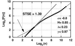
Figure 2: Detrended Fluctuation Analysis of the MCAfv time series of a healthy subject. The slope of the the grey line gives the value of the short time scaling exponent STSE. The parameters of the fit (2) are shown in the right bottom corner of the graph.

Figure 3: DFA of a time series generated by the cerebral blood flow map (CBFM) with the following parameters: $b=0.10$, $a=0.05$, $\tau=15$ and $\sigma=0.20$ (the time series was scaled to facilitate comparison with the DFA shown in Fig. 2).

Figure 4: DFA of the MCAfv time series of a migraineur without aura. The time series was recorded during a headache-free interval.

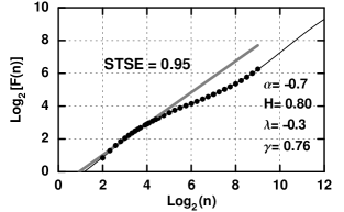
Figure 5: DFA of the MCAfv time series of a migraineur with aura. The measurement was performed during a headache.

Figure 6: DFA of a time series generated by the CBFM with the following parameters: $b=0.40$, $a=0.35$, $\tau=15$ and $\sigma=0.20$.

References

- Bassingthwaighte et al. (1994) J. B. Bassingthwaighte, L. S. Liebovitch, and B. J. West, Fractal Physiology (Oxford University Press, Oxford, 1994).
- Peng et al. (1993) C. K. Peng, J. Mistus, J. M. Hausdorff, S. Havlin, H. E. Stanley, and A. L. Goldberger, Phys. Rev. Lett. 70, 1343 (1993).
- Goldberger (1999) A. L. Goldberger, Nonlinear Dynamics, Fractals, and Chaos Theory: Implications for Neuroautonomic Heart Rate Control in Health and Disease (World Health Organization, 1999).
- Hausdorff et al. (1995) J. M. Hausdorff, C. K. Peng, Z. Ladin, J. Y. Wei, and A. L. Goldberger, J. Appl. Physiol. 78, 349 (1995).
- Hausdorff et al. (1997) J. M. Hausdorff, S. L. Mitchell, R. Firtion, C. K. Peng, M. E. Cudkowicz, J. Y. Wei, and A. L. Goldberger, J. Appl. Phys. pp. 262–269 (1997).
- West and Griffin (1998) B. J. West and L. Griffin, Fractals 6, 101 (1998).
- Peng et al. (2000) C.-K. Peng, J. M. Hausdorff, and A. L. Goldberger, Self-Organized Biological Dynamics and Nonlinear Control (Cambridge University Pres, 2000), chap. 3, pp. 66–96.
- Heistad and Kontos (1983) D. D. Heistad and H. A. Kontos, Cerebral Circulation (Am. Physiol. Soc., Bethesda, MD, 1983), chap. 5, pp. 137–182.
- Paulson et al. (1990) O. B. Paulson, S. Strandgaard, and L. Edvinsson, Cerebrovasc. Brain Metab. Res. 2, 161 (1990).
- Cutrer et al. (2000) F. M. Cutrer, A. O’Donnell, and M. S. S. del Rio, Neurology 55, S36 (2000).
- Ferrari (1998) M. D. Ferrari, Lancet 351, 1043 (1998).
- Goadsby et al. (2002) P. J. Goadsby, R. B. Lipton, and M. D. Ferrari, N. Engl J Med 346, 257 (2002).
- Goadsby (2001) P. J. Goadsby, Wolff’s headache and other head pain (Oxford University Press, 2001), chap. Pathophysiology of headache, pp. 57–72.
- Battistella (1990) P. A. Battistella, Headache 30, 646 (1990).
- Mirza (1998) M. Mirza, Acta Neurol Belg 98, 190 (1998).
- Olsen and Lassen (1989) T. S. Olsen and N. Lassen, Headache 31, 49 (1989).
- Heckmann (1998) J. G. Heckmann, Cephalalgia 18, 133 (1998).
- Zhang et al. (1999) R. Zhang, J. H. Zuckerman, C. Giller, and B. D. Levine, Am. J. Physiol. 274, H233 (1999).
- Keunen et al. (1994) R. W. M. Keunen, H. Pijlman, H. F. Visee, J. H. R. Vliegen, D. L. T. Tavy, and C. J. Stam, Neurophys. Res. 16, 353 (1994).
- Keunen et al. (1996) R. W. M. Keunen, J. H. R. Vliegen, C. J. Stam, and D. L. T. Tavy, Ultrasound Med. Biol. 22, 353 (1996).
- Rossitti and Stephensen (1994) S. Rossitti and H. Stephensen, Acta Physio. Scand. 151, 191 (1994).
- West et al. (1999) B. J. West, R. Zhang, A. W. Sanders, J. H. Zuckerman, and B. D. Levine, Phys. Rev. E 59, 3492 (1999).
- West et al. (2003) B. J. West, M. Latka, M. Glaubic-Latka, and D. Latka, Physica A 318, 431 (2003).
- of the International Headache Society (1988) H. C. C. of the International Headache Society, Cephalalgia 8, 10 (1988).
- Peng et al. (1994) C. K. Peng, S. V. Buldyrev, S. Havlin, M. Simons, H. E. Stanley, and A. L. Goldberger, Phys. Rev. E 49, 1685 (1994).
- Glass and Mackey (1988) L. Glass and M. C. Mackey, From Clocks to Chaos, The Rhythms of Life (Princeton University Pres, NJ, 1988).
- Afra et al. (2000) J. Afra, A. P. Cecchini, P. S. Sandor, and J. Schoenen, Clinical Neurophysiology 111, 1124 (2000).