Why current-carrying magnetic flux tubes gobble up plasma and become thin as a result

Abstract

Suppose an electric current $I$ flows along a magnetic flux tube that has poloidal flux $\psi$ and radius $a=a(z)$ where $z$ is the axial position along the flux tube. This current creates a toroidal magnetic field $B_{\phi}.$ It is shown that, in such a case, non-linear, non-conservative $\mathbf{J\times B}$ forces accelerate plasma axially from regions of small $a$ to regions of large $a$ and that this acceleration is proportional to $\partial I^{2}/\partial z$. Thus, if a current-carrying flux tube is bulged at, say, $z=0$ and constricted at, say, $z=\pm h$, then plasma will be accelerated from $z=\pm h$ towards $z=0$ resulting in a situation similar to two water jets pointed at each other. The ingested plasma convects embedded, frozen-in toroidal magnetic flux from $z=\pm h$ to $z=0$. The counter-directed flows collide and stagnate at $z=0$ and in so doing (i) convert their translational kinetic energy into heat, (ii) increase the plasma density at $z\approx 0$, and (iii) increase the embedded toroidal flux density at $z\approx 0$. The increase in toroidal flux density at $z\approx 0$ increases $B_{\phi}$ and hence increases the magnetic pinch force at $z\approx 0$ and so causes a reduction of  $a(0)$. Thus, the flux tube develops an axially uniform cross-section, a decreased volume, an increased density, and an increased temperature. This model is proposed as a likely hypothesis for the long-standing mystery of why solar coronal loops are observed to be axially uniform, hot, and bright. It is furthermore argued that a small number of tail particles bouncing between the approaching counterstreaming plasma jets should be Fermi accelerated to extreme energies. Finally, analytic solution of the Grad-Shafranov equation predicts that a flux tube becomes axially uniform when the ingested plasma becomes hot and dense enough to have  $2\mu_{0}n\kappa T/B_{pol}^{2}=\ (\mu_{0}Ia(0)/\psi)^{2}/2$; observed coronal loop parameters are in reasonable agreement with this relationship which is analogous to having $\beta_{pol}=1$ in a tokamak.

year number number identifier

LABEL:FirstPage1 LABEL:LastPage#1

I   Introduction

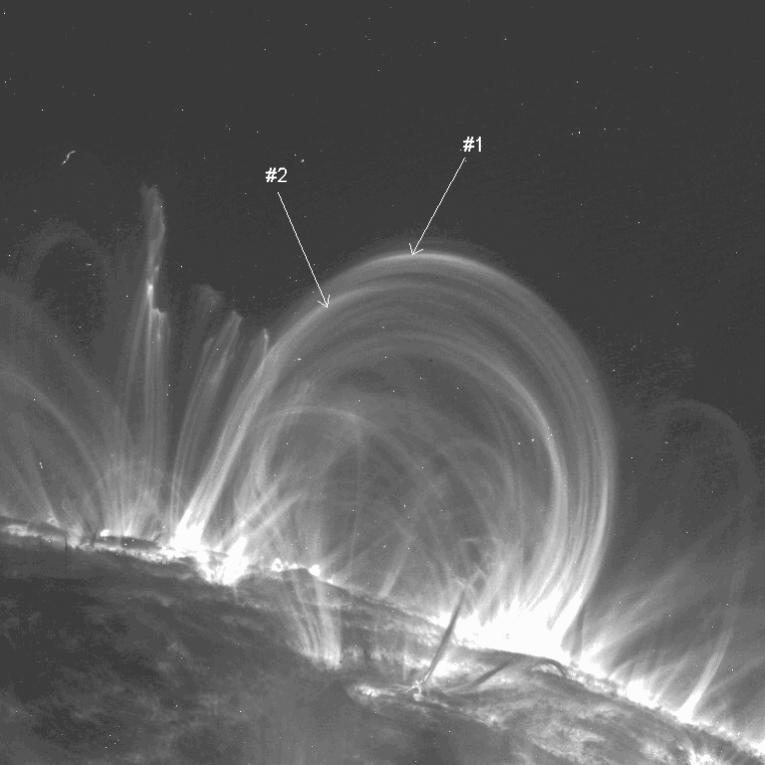
A long standing mystery in solar physics is why solar coronal loops typically have an axially uniform cross-section Klimchuk:2000 ; i.e., a filamentary shape. This issue has been made especially pressing by recent TRACE (Transition Region and Coronal Explorer ) spacecraft soft x-ray images which show a multitude of highly-defined axially uniform loops Aschwanden:2000 ; for example, see Fig. 1. Axial uniformity of flux tubes  is also commonly observed in laboratory experiments, for example, in recent simulations of solar prominences Hansen:2001 .

Figure 1: TRACE soft X-ray photo showing axial uniformity of coronal loops (image courtesy Lockheed Martin Space and Astrophysics Lab). As discussed in the text, the slight wrapping of flux tube #1 around flux tube #2 indicates that net currents flow along the flux tubes.

This paper argues that axial uniformity is the result of a rather complex sequence of events which occur whenever an electric current $I$ is made to flow along an initially axially non-uniform, current-free, axisymmetric magnetic flux tube (a process corresponding to injection of magnetic helicity into the flux tube). The sequence of events occurs even when $I$ is modest, i.e., even when the flux tube is only slightly twisted.

Figure 2: (a) Potential (i.e., current-free) coronal loop above solar surface with corresponding subsurface field and source currents. The cross-section of the loop is largest at the top of the loop where the magnetic field is weakest; (b) straight cylindrical representation of coronal loop used in model.

The typical arched shape of coronal loops is shown schematically in Fig. 2a; to make the analysis tractable we will assume that the loop is straight as sketched in Fig. 2b. However, in order to retain an important aspect of the arched shape, we will allow the length of the straight loop to vary to take into account possible variability in the length of the arched loop. The Fig. 2b geometry will be characterized by a straight cylindrical coordinate system $\{r,\phi,z\}$ where $z$ refers to the direction along the loop axis, $\phi$ is the azimuthal direction about the axis, and $r$ is the distance from the axis. The $\phi$ direction is called the toroidal direction and the $r,z$ directions are called poloidal. Flux coordinates will also be used when appropriate. This poloidal/toroidal nomenclature is formally the same as that used for tokamaks, but the configuration should not be confused with a tokamak as there are no closed poloidal field lines. The current $I$ will be assumed to be relatively small so that the poloidal field magnitude $\sim B_{z}$ is always much larger than $B_{\phi}$ in which case the flux tube is only slightly twisted. We note that this straight cylindrical approximation of flux tube geometry has been used in many previous studies of flux tube equilibria, especially force-free equilibria (for example, see Refs.Parker:1979 ; Browning:1983 ; Zweibel:1985 ; Browning:1989 ; Lothian:1989 ; VanderLinden:1999 ). However, the analysis presented here differs substantively from these previous studies because our analysis does not begin by assuming existence of an equilibrium. Instead, our analysis characterizes the dynamics that lead to an equilibrium and shows how the resulting equilibrium is intimately related to these dynamics. Furthermore, our analysis takes into account the non-force-free aspects of the equilibrium (i.e., finite pressure gradients) and shows that these finite $\beta$ aspects are of vital importance to the axial uniformity of the equilibrium.

Because of the assumed axisymmetry in Fig. 2b, the magnetic field can be expressed as

$$\mathbf{B=}\frac{1}{2\pi}\left(\nabla\psi\times\nabla\phi+\mu_{0}I\nabla\phi\right)$$ (1)

where $\nabla\phi=\hat{\phi}/r$ and

$$\psi(r,z,t)=\int_{0}^{r}B_{z}(r^{\prime},z,t)2\pi r^{\prime}dr^{\prime}$$ (2)

is the poloidal flux. Axial non-uniformity corresponds to having $\partial\psi/\partial z\neq 0\$ and axial bulging corresponds to having $\psi^{-1}\partial^{2}\psi/\partial z^{2}>0.$ The current $I$ is similarly given as

$$I(r,z,t)=\int_{0}^{r}J_{z}(r^{\prime},z,t)2\pi r^{\prime}dr^{\prime}$$ (3)

and is related to the toroidal field by Ampere’s law, i.e., $\mu_{0}I=2\pi rB_{\phi}.$ The current rise time $\tau$ is assumed to be sufficiently slow that Alfvén wave propagation effects are unimportant i.e., it is assumed that $v_{A}\tau>>h$ where $2h$ is the length of the flux tube. The current thus flows as in an electric circuit so that there are no retarded time or radiation effects. Taking the curl of Eq.(1) shows that the current density associated with the magnetic field is

$$\mathbf{J=-}\frac{r^{2}\nabla\phi}{2\pi\mu_{0}}\nabla\cdot\left(\frac{1}{r^{2}}\nabla\psi\right)+\frac{1}{2\pi}\nabla I\times\nabla\phi.$$ (4)

Controversy exists regarding the properties of $I(r,z)$ external to the current-carrying flux tube$.\$ Some authors Parker:1996 ; Linton:2001 argue that $I$ must vanish outside the flux tube while others Mok:1997 ; Longcope:2000 ; Chen:2001 ; Melrose:1995 argue that $I$ should be finite outside. If one insists that $I$ vanishes outside the flux tube so that there is no net current in a flux tube, the flux tube acts like a coaxial cable (i.e., a center conductor sheathed by a coaxial outer conductor carrying equal and opposite current). This neutralized current configuration has $B_{\phi}=0$ external to the flux tube and so cannot produce magnetic forces on external currents. Adjacent neutralized flux tubes thus cannot exert forces on each other and so will not mutually interact, just like adjacent coaxial cables will not mutually interact. Furthermore, sections at different axial positions along the length of a neutralized flux tube cannot interact via magnetic forces. The lack of interaction between sections at different axial positions along the length of a neutralized flux tube means that such a flux tube cannot undergo a kink instability since a kink instability involves relaxing to the state of lowest mutual interaction energy between loop segments (similarly, a coaxial cable will not undergo a kink instability since there is no force between axially separated segments).

In contrast, having a net current (i.e., being non-neutralized) implies existence of an external potential magnetic field $B_{\phi}$ $\sim I/r$ outside of the flux tube just like the magnetic field external to an ordinary current-carrying wire. An individual flux tube with net current can kink since, if its axis bends, there will be forces between sections at different axial positions. Two flux tubes, each carrying net current, will experience mutual interaction forces due to the $B_{\phi}$ of one flux tube interacting with the current of the other flux tube. Thus, two adjacent flux tubes each with net current will tend to wrap around each other as shown in Fig. 2a of Ref.Lau:1996 since the axis of each flux tube will be affected by the $B_{\phi}$ of its neighbor. Since we are assuming here that $B_{\phi}<<B_{z}$ this wrapping will be very slight. Examination of the loop structures #1 and #2 denoted by arrows in Fig.1 show that these two structures do indeed wrap around each other slightly (on the left, loop #1 is to the rear of loop #2; on the right, the two loops appear to be in the plane of the photo).

Based on the observations that kinks do occur in solar structures and that coronal loops do show evidence of wrapping we will assume in this paper that net current does flow in a flux tube, i.e., that the current is non-neutralized. This assumption is additionally supported by recent work by Feldman Feldman:2002 and by WheatlandWheatland:2000 who, after careful analysis of a variety of observational evidence, have concluded that net currents do flow.

The assumption of net current means that we are allowing flux tubes to interact with each other via magnetic forces. However, since the effect of this interaction is to alter the  three dimensional locus of a flux tube axis, and since we are invoking the straight axis approximation (i.e. using Fig. 2b to represent Fig. 2a), we are removing from consideration the evolution of the three dimensional locus of the flux tube axis. The straight axis approximation is thus analogous to a kinematics problem where one works in the center of mass frame of a body and so removes from consideration external body forces that change the location of the center of mass.

The dynamics of the configuration are governed by the combination of the magnetohydrodynamic (MHD) equation of motion

$$\rho\frac{d\mathbf{U}}{dt}=\mathbf{J\times B}-\nabla P$$ (5)

and the induction equation

$$\frac{\partial\mathbf{B}}{\partial t}=\nabla\times\left(\mathbf{U\times B}\right)$$ (6)

where the latter is obtained from the curl of the ideal MHD Ohm’s law

$$\mathbf{E+U\times B=}0.$$ (7)

The flux tube ends are at $z=\pm h$ and the flux tube middle is at $z=0.$ The flux tube is assumed to be initially current-free so that initially $I=0.$ The field in the flux tube is thus initially potential (i.e., $\nabla\times\mathbf{B=}0$ initially) and the source currents generating this potential field are external to the flux loop and, as sketched in Fig. 2a, are assumed to be below the solar surface. Thus the initially potential coronal loop sketched in Fig. 2a will have a magnetic field that is stronger at the footpoints than at the arch top because the arch top is further from the source currents. This means that the initial current-free flux tube will be bulged at the top because the magnetic field is weaker there. In the straight geometry representation given by Fig.2b, the bulging at the arch top corresponds to having the initially potential poloidal field stronger at $z=\pm h$ than at $z=0$ and the flux tube diameter larger at $z=0$ than at $z=\pm h.$

The sequence of events that occurs when the current is ramped up to a steady-state will be shown to consist of the following three stages:

1. The first stage consists of a twisting of the magnetic field about the $z$ axis in Fig. 2b together with an associated transient toroidal plasma velocity $U_{\phi}$. This stage is incompressible and maintains the flux tube poloidal profile, i.e., $\psi(r,z)$ is unchanged and the flux tube remains bulged. The velocity $U_{\phi}$ is proportional to $z\partial I/\partial t$ and the toroidal acceleration is proportional to $z\partial^{2}I/\partial t^{2}.$

2. The second stage involves generation of axial plasma flows. These flows go from $z=\pm h$ where the flux tube diameter is small to $z=0$ where the diameter is large. The flows are driven by a $z$-directed force which is proportional to $-\partial I^{2}/\partial z.$ This axial force is a nonlinear function of $I$ in contrast to the first stage toroidal acceleration which is a linear function of $I.$

3. The third stage involves stagnation of the converging flows at $z=0$ resulting in plasma heating as the flow kinetic energy is converted into heat (thermalized). There is also an accumulation of convected toroidal flux at $z=0$ which leads to an enhancement of the pinch force at $z=0$. The enhanced pinch force squeezes the flux tube diameter at $z=0$ so that the flux tube approaches axial uniformity, i.e., $\partial\psi/\partial z\rightarrow 0.$ Ultimately, an axially uniform flux  tube loaded with hot plasma results.

II Lack of equilibrium for arbitrarily specified magnetic fields

Arbitrarily specified magnetic fields do not, in general, have associated MHD equilibria, i.e., in general, no pressure $P(\mathbf{r)}$ exists which satisfies

$$\mathbf{J\times B}=\nabla P$$ (8)

for arbitrarily specified $\mathbf{B(r).}$ The essential physics underlying this assertion is that $\nabla\times\nabla P$ is identically zero whereas $\nabla\times\left(\mathbf{J\times B}\right)$ is not necessarily zero, i.e., $\nabla P$ is always a conservative force whereas $\mathbf{J\times B}$ is in general non-conservative. A non-conservative force has an associated torque and since a pressure gradient cannot balance a torque, no equilibrium is possible when $\nabla\times\left(\mathbf{J\times B}\right)$ is finite.

Figure 3: Poloidal flux surfaces of a magnetic field configuration for which no finite pressure gradient MHD equilibrium is possible.

As a specific example that equilibria do not exist for arbitrarily specified magnetic field configurations, consider the simple situation sketched in Fig. 3. We assert that no MHD equilibrium is possible for this configuration, i.e., this configuration cannot satisfy Eq. (8). This assertion is established by calculating radial pressure balance at axial locations $\ \ z_{1}$ and $z_{2}$ where the respective flux tube radii are $a$ and $b\$with $b>a.$ If satisfied, Eq. (8) imposes the requirement $\mathbf{B\cdot}\nabla P=0$ which means that   the pressure must be the same everywhere on a field line.

The poloidal component of the magnetic field is assumed to be straight, uniform, and in the $z$ direction at both $z_{1}$ and $z_{2}.$ Because the field lines are more densely packed at $z_{1}$ than at $z_{2},$ the magnetic field is such that $B_{z}(z_{1})>B_{z}(z_{2}).$ In addition, since the poloidal magnetic field is uniform at  $z_{1}$ and $z_{2},$ the toroidal current vanishes at both $z_{1}$ and $z_{2}$ [in fact, uniformity of poloidal field is more than is needed for the toroidal current to vanish as the most general requirement for the toroidal current to vanish is to have $\nabla\cdot\left(r^{-2}\nabla\psi\right)=0$].

Using $J_{\phi}=0$ the radial component of Eq.(8) is therefore

$$\partial P/\partial r=-J_{z}B_{\phi}=-\frac{\mu_{0}I}{\left(2\pi r\right)^{2}}\frac{\partial I}{\partial r}.$$ (9)

However, the toroidal component of Eq.(8) gives

$$\left(\nabla I\times\nabla\phi\right)\times\left(\nabla\psi\times\nabla\phi\right)=0$$ (10)

which implies that $I=I(\psi).$ Since the poloidal magnetic field is straight and uniform at both $\ z_{1}\$and $z_{2}$, the poloidal flux function must have the form $\psi=\psi_{0}r^{2}/a^{2}$   at $\ z_{1}$ and $\psi=\psi_{0}r^{2}/b^{2}$ at $\ z_{2}$ where $\psi_{0}$ is the flux on the surface for which $P$ vanishes and $a,b$ are the respective radii of these flux surfaces at $z_{1}$ and $z_{2}.$ The simplest non-trivial possibility for $I=I(\psi)$ is to assume that $I$ is a linear function of $\psi$ so

$$\mu_{0}I=\alpha\psi.$$ (11)

Radial pressure balance at $z=z_{1}$ thus becomes

$$\partial P/\partial r=-\frac{\alpha^{2}\psi}{\left(2\pi r\right)^{2}\mu_{0}}\frac{\partial\psi}{\partial r}=-\frac{\alpha^{2}\psi_{0}^{2}}{2\pi^{2}\mu_{0}}\frac{r}{a^{4}}$$ (12)

which can be integrated to give the on-axis pressure at $z_{1}$ to be

$$P(0,z_{1})=\int_{a}^{0}dr\partial P/\partial r=\int_{0}^{a}dr\frac{\alpha^{2}\psi_{0}^{2}}{2\pi^{2}\mu_{0}}\frac{r}{a^{4}}=\frac{\alpha^{2}\psi_{0}^{2}}{4\pi^{2}a^{2}\ \mu_{0}}.$$ (13)

However, a similar evaluation of the on-axis pressure at $z=z_{2}$ gives

$$P(0,z_{2})=\frac{\alpha^{2}\psi_{0}^{2}}{4\pi^{2}b^{2}\mu_{0}}$$ (14)

which is smaller than the on-axis pressure at $z=z_{1}$ since $b>a$. Thus, the pressure is not uniform along the on-axis field line and so the requirement $\mathbf{B}\cdot\nabla P=0$ is violated on the $z$-axis. Equation (8) is therefore not satisfied and so equilibrium does not exist. Because there is radial pressure balance but not axial pressure balance, we might expect flows to be driven from $z_{1}$ to $z_{2}.$ The situation is analogous to squeezing the end of a toothpaste tube  and having toothpaste squirt out the mouth of the tube.

III General case using flux coordinates

Let us now return to the problem of a coronal loop which is initially current-free and bulging at $z=0$, but then has an externally driven current $I$ slowly ramped up to a constant value. We define a right-handed orthogonal coordinate system based on the poloidal flux coordinates. The unit vectors of this system are

$$\mathbf{e}_{\psi} =\frac{\nabla\psi}{|\nabla\psi|}$$

$$\mathbf{e}_{\phi} =\hat{\phi}$$

$$\mathbf{e}_{Bpol} =\frac{\nabla\psi\times\nabla\phi}{|\nabla\psi\times\nabla\phi|}$$ (15)

so that $\mathbf{e}_{\psi}\rightarrow$ $\hat{r}$ and $\mathbf{e}_{Bpol}$ $\rightarrow\hat{z}$ if the field lines are straight and axial.  The form of $\mathbf{e}_{\psi}$ shows that $B_{\psi}=\mathbf{B\cdot e}_{\psi}$ is zero by definition; i.e., the magnetic field can never have a component in the direction of $\nabla\psi.$

The current density can be decomposed into the components

$$J_{\psi}=\frac{1}{2\pi}\nabla I\times\nabla\phi\cdot\frac{\nabla\psi}{|\nabla\psi|}$$ (16)

$$J_{\phi}=\mathbf{-}\frac{r}{2\pi\mu_{0}}\nabla\cdot\left(\frac{1}{r^{2}}\nabla\psi\right)$$ (17)

$$J_{Bpol}=\frac{1}{2\pi r}\frac{\nabla I\cdot\nabla\psi}{|\nabla\psi|}.$$ (18)

We now argue that $J_{\psi},J_{\phi},$ and $J_{Bpol}$ each have distinctive physics.

The component $J_{\psi}$ flows normal to flux surfaces and provides the torque that causes the plasma to rotate toroidally. This current can only be transient and is identified as the polarization current Chen:1984 . Polarization current can be thought of as being an essentially dependent quantity; that is, one first determines the amount of toroidal acceleration using an analysis that does not involve the equation of motion, and then one inserts this acceleration into the equation of motion to calculate the required polarization current. The reason for this inferior status of the toroidal component of the equation of motion is that the toroidal symmetry of the system provides a strong constraint on the dynamics. From an MHD point of view, the toroidal symmetry means that no toroidal pressure gradient can exist and also no toroidal electrostatic electric field can exist. From a particle Hamiltonian point of view, this symmetry means that the maximum excursion particles can make from a flux surface is no more than a poloidal Larmor radius Bellan:2000 , a microscopic length. The localization of particles to the vicinity of a flux surface means that there cannot be any sustained net current density in the direction normal to a flux surface and so $J_{\psi}$ is highly constrained. All that is allowed is a short-lived transient $J_{\psi}^{\ }$ having zero time-average; i.e., $J_{\psi}$ can only be an AC current. The slight bobbing back and forth of particles off of a flux surface constitutes the polarization current. Thus the plasma acts like a capacitor in the direction normal to the flux surfaces, but like a wire in the direction along the flux surfaces. As is well knownChen:1984a , the dielectric constant of the plasma “capacitor” is given by $\mu_{0}\rho c^{2}/B^{2}=c^{2}/v_{A}^{2}>>1.$ Polarization currents have an associated polarization electric field normal to the flux surface resulting from the particles making their small excursions from their nominal flux surface.

The current $I$ is assumed to be generated by some sub-surface dynamo and so its time-dependence is a prescribed quantity. This time dependence is assumed to be such that $I$ increases smoothly from zero to some finite value in a characteristic time $\tau>>h/v_{A}.$ This smooth increase can be represented by the characteristic time profile

$$I(t)=\frac{\left(\tanh(t/\tau)+1\right)}{2}I_{0}$$ (19)

so that $I=0$ for $t<<-\tau$ and $I=I_{0}$ for $t>>\tau.$ It should be noted that $\partial I/\partial t\sim 1/\cosh^{2}(t/\tau)$ which has its maximum at $t=0$ and that $\partial^{2}I/\partial t^{2}\sim-\tanh\left(t/\tau\right)/\cosh^{2}(t/\tau)$ which is positive for $t$ slightly before $t=0$ and negative for $t$ slightly after $t=0$ and then otherwise zero.

Figure 4: First stage dynamics: Top shows flux tube when $I=0.$ Bottom shows flux tube when $I$ is finite, but $\psi(r,z)$ is not yet changed from its initial potential value. The evolution from the top to the bottom situation involves toroidal rotation by a finite amount, but no poloidal flows.

III.1 First stage (ramp-up)

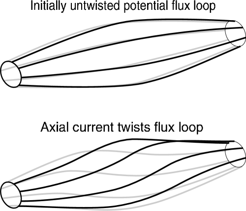
At the beginning of the first stage $I$ is zero and the flux tube is untwisted as shown in the top sketch of Fig. 4.  The toroidal component of the induction equation is

$$\frac{\partial B_{\phi}}{\partial t}=\ r\mathbf{B}_{pol}\mathbf{\cdot}\nabla\left(\frac{U_{\phi}}{r}\right)-r\mathbf{U}_{pol}\mathbf{\cdot}\nabla\left(\frac{B_{\phi}}{r}\right)-B_{\phi}\nabla\cdot\mathbf{U}_{pol}\$$ (20)

and the toroidal component of Ohm’s law can be expressed as

$$\frac{\partial\psi}{\partial t}\mathbf{+U}_{pol}\mathbf{\cdot}\nabla\psi\mathbf{=}0.$$ (21)

We will show that $\mathbf{U}_{pol}$ results from a weak non-linear force and so is negligible at times $t\sim 0$ because there has not been enough time for a significant $\mathbf{U}_{pol}$ to develop. In contrast, $U_{\phi}$ is proportional to $\partial I/\partial t$ and so $U_{\phi}$ is large at $t\sim 0\$when $\partial I/\partial t$ is at its maximum. However $U_{\phi}$ goes to zero at large times when $\partial I/\partial t\rightarrow 0.$ Thus, the time when $U_{\phi}$ is finite precedes the time when $\mathbf{U}_{pol}$ is finite. The first stage characterizes the time $t\sim 0$ when $\mathbf{U}_{pol}$ is negligible, $\psi$ is unchanged from its initial potential state, $J_{\phi}$ is negligible,   and $U_{\phi}$ is transiently finite.

Letting $s$ denote the distance along the poloidal field from the $z=0$ plane and taking into account that $\mathbf{U}_{pol}\simeq 0$, Eq.(20) may therefore be approximated at $t\sim 0$ as

$$\frac{\partial B_{\phi}}{\partial t}\simeq B_{pol}\mathbf{\ }\frac{\mathbf{\partial}U_{\phi}}{\partial s}\$$ (22)

which may be integrated with respect to $s$ to give

$$U_{\phi}\simeq\frac{s}{B_{pol}}\frac{\partial B_{\phi}}{\partial t}=\frac{\mu_{0}s}{2\pi B_{pol}r}\frac{\partial I\ }{\partial t}.$$ (23)

The finite toroidal displacement $r\Delta\phi=\int U_{\phi}dt$ is proportional to $s$ and so gives a twisting up of the flux tube as shown in the bottom sketch of Fig. 4. In fact this twisting motion is such that

$$\frac{r\Delta\phi}{B_{\phi}}=\ \frac{\ s}{\ B_{pol}\ }\$$ (24)

showing that the plasma twist is just what is required to keep the plasma frozen to the twisting magnetic field.

Equation (23) and Eq.(7) together imply the existence of an electric field in the $\nabla\psi$ direction

$$E_{\psi}=-U_{\phi}B_{pol}=-\frac{\mu_{0}s}{2\pi r}\frac{\partial I\ }{\partial t};\$$ (25)

this is the polarization electric field. The toroidal component of the equation of motion is

$$\rho\frac{\partial U_{\phi}}{\partial t}\simeq-J_{\psi}B_{pol}$$ (26)

since $B_{\psi}=0$. Thus, the current normal to a flux surface is

$$J_{\psi}=-\frac{\rho}{B_{pol}}\frac{\partial U_{\phi}}{\partial t}=\frac{\rho}{B_{pol}^{2}}\frac{\partial E_{\psi}}{\partial t}=-\frac{\rho}{B_{pol}^{2}}\frac{\mu_{0}s}{2\pi r}\frac{\partial^{2}I\ }{\partial t^{2}}.$$ (27)

Equation (27) clearly shows that $J_{\psi}$ is indeed the polarization current and that $J_{\psi}$ is essentially a dependent quantity since it is proportional to $\partial^{2}I/\partial t^{2}.$ The polarization current is transient and, for positive $s,$ is first negative and then positive (and vice versa for negative $s$). Both $U_{\phi}$ and the polarization current $J_{\psi}$ vanish when $I$ is in steady state. The chain of dependence is such that the induction equation first determines $U_{\phi}$ which then determines $J_{\psi}\$via the equation of motion. For a long, thin flux tube, $s\simeq z,$ $B_{pol}\simeq B_{z}$, and the $\psi$ direction is approximately the $r$ direction. For $t>>\tau$, the poloidal current $I$ is in steady state and so $U_{\phi}=0\$for $t>>\tau.$

III.2 Second stage (steady $I,$ development of finite $\mathbf{U}_{pol}$)

Since $I$ is constant in the second stage, $U_{\phi}\$and $J_{\psi}$ are both zero. Equation (16) shows that $J_{\psi}=0$   implies $I=I(\psi)\$in which case surfaces of constant $\psi(r,z)$ are also surfaces of constant $I(r,z)$. At the beginning of the second stage, $\mathbf{U}_{pol}$ has not yet developed and so $\psi(r,z)$ is assumed to be unchanged from its initial potential (vacuum) state, i.e., the poloidal profile of the flux surfaces is not yet deformed. Thus, $J_{\phi}=\mathbf{-}r\left(2\pi\mu_{0}\right)^{-1}\nabla\cdot\left(r^{-2}\nabla\psi\right)=0$ at the beginning of the second stage.

We now consider the dynamics. The magnetic force can be decomposed into toroidal and poloidal components as follows:

$$\mathbf{J\times B}=\mathbf{J}_{pol}\mathbf{\times B}_{pol}+\mathbf{J}_{pol}\mathbf{\times B}_{tor}+\mathbf{J}_{tor}\mathbf{\times B}_{pol}.$$ (28)

However, $\mathbf{J}_{pol}\mathbf{\times B}_{pol}$ $=\mathbf{J}_{\psi}\mathbf{\times B}_{pol}=0$ and $\mathbf{J}_{tor}=J_{\phi}\hat{\phi}=0$ so that the magnetic force at the beginning of the second stage reduces to

$$\mathbf{J\times B}=\mathbf{J}_{pol}\mathbf{\times B}_{tor}=\frac{1}{2\pi}\left(\nabla I\times\nabla\phi\right)\times\frac{\mu_{0}I}{2\pi}\nabla\phi=-\frac{\mu_{0}}{8\pi^{2}r^{2}}\nabla I^{2}.$$ (29)

Since the curl of the magnetic force given in Eq.(29) is non-zero, it is impossible for a pressure gradient to balance the magnetic force at this stage. The $z$ component of the magnetic force is

$$\ \left(\mathbf{J\times B}\right)_{z}=-\frac{\mu_{0}}{8\pi^{2}r^{2}}\frac{\partial I^{2}}{\partial z}$$ (30)

which is independent of the sign of $I$, nonlinear in $I,$ and such as to accelerate plasma from regions where the diameter of the current channel is small to regions where the diameter is large. In the case of a flux tube which is bulged in the middle, the force given in Eq.(30) will accelerate plasma axially from $z=\pm h$ towards $z=0$.

The force given in Eq.(30) vanishes at $r=0$ since $I\sim r^{2}$ for small $r.$ However, axially localized radial force balances will quickly develop between the magnetic force and the radial pressure gradient as discussed in Section II. The resulting radial force balance will produce an axially non-uniform pressure and so there will also be an axial force due to the axial pressure gradient.

Specifically, radial pressure balance means that

$$\frac{\partial P}{\partial r}=-J_{z}B_{\phi}=-\frac{\mu_{0}}{8\pi^{2}r^{2}}\frac{\partial I^{2}}{\partial r}.$$ (31)

This radial pressure balance equation is not integrable for arbitrary $I(r,z)$, but to get an idea for the general behavior we make the assumption that $I\sim r^{2}$ which is integrable. Thus, assuming $I(r,z)=\left(r/a(z)\right)^{2}I_{0}$ where $I_{0}$ is the total current flowing in the flux tube of radius $a(z),$ Eq.(31) can be integrated to give

$$P(r,z)=\frac{\mu_{0}I_{0}^{2}}{4\pi^{2}a^{2}\ \ }\left(1-\frac{r^{2}}{a^{2}}\right)$$ (32)

so that

$$-\frac{\partial P}{\partial z}=\frac{\mu_{0}I_{0}^{2}}{\pi^{2}a^{3}\ \ }\left(\frac{1}{2}-\frac{r^{2}}{a^{2}}\right)\frac{\partial a}{\partial z}$$ (33)

is the axial force due to the axial non-uniformity of the pressure.

Using $I(r,z)=I_{0}r^{2}/a^{2}$ to estimate the axial component of the magnetic force gives

$$\left(\mathbf{J\times B}\right)_{z}=-\frac{\mu_{0}}{8\pi^{2}r^{2}}\frac{\partial I^{2}}{\partial z}=\ \frac{\mu_{0}I_{0}^{2}}{2\pi^{2}}\ \frac{r^{2}}{a^{5}}\frac{\partial a}{\partial z}.$$ (34)

The total force in the $z$ direction for this case is thus

$$F_{z} =\ \left(\mathbf{J\times B}\right)_{z}-\frac{\partial P}{\partial z}$$

$$=\ \frac{\mu_{0}I_{0}^{2}}{2\pi^{2}a^{3}\ \ }\left(1-\frac{r^{2}}{\ a^{2}}\right)\frac{\partial a}{\partial z}.$$ (35)

This total force is peaked on the axis and has magnitude

$$F_{z}\sim-\frac{\partial}{\partial z}\left(\left[\frac{B_{\phi}^{2}}{\mu_{0}}\right]_{r=a}\right).\$$ (36)

This force will result in axial flows from $z=\pm h$ to $z=0$ with velocities that are of the order of $B_{\phi}(r=a,z=\pm h)/\sqrt{\mu_{0}\rho}.$ Because $J_{\phi}=0$, the behavior is essentially identical to the situation where $\psi=0$ and so the flow acceleration mechanism is similar to that discussed in Refs. Maeker:1955 -Bellan:1992 which consider MHD arc-jets for the situation of purely toroidal magnetic fields.

Figure 5: Evolution of flux tube due to effect of $\mathbf{J\times B}$ force when $I$ is constant. Solid line shows initial constant $\psi(r,z)$ flux surface, dashed line shows same flux surface at a later time. Fluid elements (shown hatched) are pushed axially towards $z=0$ while staying on the same constant $\psi$ surface. The resulting fluid flows collide at the $z=0$ plane where they thermalize their directed kinetic energy. Toroidal flux and mass accumulate at the $z=0$ layer also. The accumulation of toroidal flux at $z=0$ increases $B_{\phi}$ there and so pinches down the flux tube diameter causing the flux tube to become axially uniform.

III.3 Third stage (convection of toroidal flux, fluid stagnation, heating, compression)

The force given by Eq.(29) has a finite curl and so cannot be balanced by a pressure gradient so long as the original potential profile of $\psi(r,z)$ is maintained. Thus, the only way for an equilibrium to develop is for the profile of $\psi(r,z)$ to change. This is clearly evident from the discussion in Section III(B): Eq.(35) shows that axial equilibrium can only occur if $\partial a/\partial z\rightarrow 0$.

Attainment of equilibrium involves several inter-related hydrodynamic, magnetic, and thermodynamic phenomena which are shown schematically in Fig. 5. The solid lines in Fig. 5 show a constant $\psi$ surface at an early time and the dashed lines show this constant $\psi$ surface at a later time. Typical fluid elements are shown as hatched parallelograms (cross-sections of toroids) and the motion of these elements is seen to consist of both axial and radial motion such that each fluid element stays on its own constant $\psi$ surface. The non-conservative nature of the $\mathbf{J\times B}$ force is shown in Fig. 5 by the longer length at larger $|z|$ of the arrows representing $\mathbf{J\times B}$. The axial motion corresponds to plasma flows which ingest plasma at $z=\pm h$, travel towards $z=0,$ and then converge and stagnate at $z=0\$like two water jets pointed at each other. The stagnation converts the flow kinetic energy into heat and simultaneously increases the plasma density at $z=0$ as plasma accumulates there. Thus pressure increases at $z=0$. Furthermore, toroidal flux embedded in the plasma is convected by the axial flows and so there will also be an accumulation of toroidal flux at $z=0$. This means that the density of the toroidal flux will also increase at $z=0,$ i.e., $B_{\phi}$ will increase in the vicinity of $z=0.$

The increase in $B_{\phi}$ can be established more rigorously by considering Eq.(20) in the vicinity of $z=0$ and taking into account that (i) $U_{\phi}=0$ since $I$ is constant, (ii) $\mathbf{U}_{pol}\rightarrow 0$ at $z=0$ since the flow stagnates at $z=0,$ and (iii) $\nabla\cdot\mathbf{U}_{pol}<0$ near $z=0$ since the flows are converging at $z=0.$ Thus,  Eq.(20) in the vicinity of $z=0\,$ reduces to

$$\frac{\partial B_{\phi}}{\partial t}\simeq\ -B_{\phi}\nabla\cdot\mathbf{U}_{pol}$$ (37)

which shows that $B_{\phi}$ must increase since $\nabla\cdot\mathbf{U}_{pol}<0$ (we note that amplification of a magnetic field by a converging flow has previously been discussed in Ref.Polygiannakis:1999 but has not otherwise received much attention). In the vicinity of the stagnation layer at $z=0$, the continuity equation reduces to

$$\frac{1}{\rho}\frac{\partial\rho}{\partial t}=-\nabla\cdot\mathbf{U}_{pol}$$ (38)

which can be combined with the induction equation to give

$$\frac{\partial B_{\phi}}{\partial t}\simeq\frac{B_{\phi}}{\rho}\frac{\partial\rho}{\partial t}$$ (39)

showing that $B_{\phi}$ increases in  proportion to the increase in mass density at the stagnation layer. Since $I$ is constant and $2\pi rB_{\phi}=\mu_{0}I$  the current channel radius in the vicinity of the stagnation layer must decrease as $B_{\phi}$ increases to keep $rB_{\phi}\$constant. Thus, the bulge of the current channel must diminish as sketched in Fig. 5 and, because $I=I(\psi)$, the bulge of the constant $\psi$ surfaces must also diminish. The result is that the flux tube tends to become axially uniform, hot, and dense.

III.4 Changes in length

Making the flux tube axially uniform increases $\mathbf{B}_{pol}$ because squeezing the poloidal flux surfaces together results in a larger field. Since $B_{pol}\sim B_{z}\$ is much larger than $B_{\phi}$, it would seem that too much energy would have to be invested into squeezing the poloidal flux surfaces together. However, if we recall that the loop is really arched and allow the loop length to change in such a way that $\int\mathbf{B}_{pol}\cdot d\mathbf{l}$ remains constant where the line integral is over the length of the loop, then the loop length $2h$ will become shorter as $\mathbf{B}_{pol}$ increases. If $\int\mathbf{B}_{pol}\cdot d\mathbf{l=}const\mathbf{.,}$ the stored energy in the poloidal field is

$$W_{pol} =\frac{1}{2\mu_{0}}\int B_{pol}^{2}\ d\mathbf{l\cdot}d\mathbf{s}$$

$$=\frac{1}{2\mu_{0}}\int\mathbf{B}_{pol}\cdot\ d\mathbf{l\ }\int\mathbf{B}_{pol}\cdot d\mathbf{s}$$

$$=\frac{\psi}{2\mu_{0}}\int\mathbf{B}_{pol}\cdot\ d\mathbf{l\ }\$$

$$=const.$$ (40)

It is reasonable to assume that $\int\mathbf{B}_{pol}\cdot d\mathbf{l}$ remains constant, because $\mathbf{B}_{pol}$ is produced by currents external to the flux tube (e.g., by the subsurface currents sketched in Fig. 2a). These source currents may be assumed to stay constant on the time scale during which the flux tube undergoes stages 1-3. If one follows the poloidal field along its entire length both above and below the solar surface, then it must satisfy Ampere’s law

$$\mu_{0}I_{ext} =\oint\mathbf{B}_{pol}\cdot d\mathbf{l}$$

$$=\int_{loop}\mathbf{B}_{pol}\cdot d\mathbf{l+}\int_{subsfc}\mathbf{B}_{pol}\cdot d\mathbf{l}$$ (41)

where the contour consists of the loop above the surface and, in addition, the subsurface portion; the contour links links the subsurface source current system denoted as $I_{ext}$. It seems reasonable to assume that the subsurface field remains invariant during stages 1-3 and so $\int_{loop}\mathbf{B}_{pol}\cdot d\mathbf{l}$ must also remain constant.

Thus, as the poloidal field lines squeeze together to make the flux tube axially uniform, the flux tube becomes shorter in such a way as to keep the energy stored in the poloidal field constant. In this manner, no work needs to be done to squeeze the poloidal flux surfaces together. One can imagine that the “field line tension” of the poloidal field shortens the length of the loop as the poloidal field is made stronger when the poloidal flux surfaces are squeezed together.

III.5 Ultimate beta

The $z-$directed force given by Eq.(30) can be written as

$$F_{z}=-\frac{\partial}{\partial z}\left(\frac{B_{\phi}^{2}}{\mu_{0}}\right).$$ (42)

The quantity $B_{\phi}^{2}/\mu_{0}$ can be considered as an effective potential energy and so the fact that $B_{\phi}^{2}/\mu_{0}$ is large at $z=\pm h$ and small at $z=0$ means that there is an effective potential well which the plasma falls down as it moves from $z=\pm h$ to $z=0$. The order of magnitude of the resulting flow velocity is given by the reduction in potential energy due to the plasma falling down the slopes of the well and so the resulting flow velocity will be $U_{z}^{2}\simeq B_{\phi}^{2}/\mu_{0}\rho$ where $B_{\phi}^{2}$ is evaluated at $z=\pm h$ where $B_{\phi}^{2}$ is largest. Thus, the flow velocity is of the order of the Alfvén velocity calculated using the toroidal field (this is much smaller than the Alfvén velocity calculated using the poloidal field on the assumption that the flux tube is only slightly twisted). At the stagnation layer the converging flow velocity is thermalized and so the plasma pressure at the stagnation layer will be of the order of $P=nm_{i}v_{Ti}^{2}+nm_{e}v_{Te}^{2}\simeq\rho U_{z}^{2}=\left[B_{\phi}^{2}/\mu_{0}\right]_{z=\pm h}.$ Assuming that $B_{\phi}<<B_{pol}$, the plasma $\beta$ resulting from flow stagnation is therefore

$$\beta\simeq\frac{2\mu_{0}P}{B_{pol}^{2}}=2\frac{B_{\phi}^{2}}{B_{pol}^{2}}=\left(\frac{\mu_{0}I}{\psi\ }\right)^{2}\frac{a^{2}}{2\ }$$ (43)

where $a$ is the radius of the flux tube and $\psi=B_{pol}\pi a^{2}.$ Using the definition $\alpha=\mu_{0}I/\psi$ then

$$\beta=\alpha^{2}a^{2}/2$$ (44)

is the value of $\beta$ resulting from flow stagnation.

The diminishing of the bulge squeezes together the poloidal field so that there will be a finite $J_{\phi}$, but if the flux tube is squeezed to the point of being axially uniform, then $J_{\phi}$ vanishes again. Thus $J_{\phi}$ starts out by being zero, becomes finite, and then becomes zero again if and when the flux tube becomes straight.

If an equilibrium is established then $\mathbf{J\times B}=\nabla P\$which implies $\mathbf{B\cdot}\nabla P\mathbf{=}0$ and $P=P(\psi).$ We define $\psi_{0}$ as the flux surface on which $P$ vanishes and $\bar{\psi}(r,z)=\psi(r,z)/\psi_{0}$ as the normalized flux so that

$$P(\psi)=(1-\bar{\psi})P_{0}$$ (45)

where $P_{0}$ is the on-axis pressure. The equilibrium equation $\mathbf{J\times B}=\nabla P$ can then be written in Grad-ShafranovGrad-Shafranov form as

$$r\frac{\partial}{\partial r}\left(\frac{1}{r}\frac{\partial\bar{\psi}}{\partial r}\right)+\frac{\partial^{2}\bar{\psi}}{\partial z^{2}}+\alpha^{2}\bar{\psi}=2\frac{r^{2}}{a_{0}^{2}}\frac{\beta}{a_{0}^{2}}\$$ (46)

where $a_{0}$ is the flux tube radius at $z=0$ and $\beta$ is defined in terms of the mean axial field at $z=0,$ i.e., $\beta=2\mu_{0}P_{0}/\left(\psi_{0}/\pi a_{0}^{2}\right)^{2}.$ The general solution to Eq.(46) is

$$\bar{\psi}(r,z)=2\frac{r^{2}}{a_{0}^{2}}\frac{\beta}{\ \ \alpha^{2}a_{0}^{2}}+\gamma\chi(r,z)$$ (47)

where $\chi(r,z)$ is any solution to the homogeneous equation

$$r\frac{\partial}{\partial r}\left(\frac{1}{r}\frac{\partial\chi}{\partial r}\right)+\frac{\partial^{2}\chi}{\partial z^{2}}+\alpha^{2}\chi=0\$$ (48)

and $\gamma$ is a constant to be determined. The condition $\bar{\psi}(r,z)=1$ when $z=0$ and $r=a_{0}$ fixes $\gamma$ so that the general solution to the Grad-Shafranov equation is thus

$$\bar{\psi}(r,z)=\ \frac{2\beta r^{2}}{\ \alpha^{2}a_{0}^{4}}+\left(1-\frac{2\beta}{\ \ \alpha^{2}a_{0}^{2}}\right)\frac{\chi(r,z)}{\chi(a_{0},0)}.$$ (49)

If $\beta=\alpha^{2}a_{0}^{2}/2$ then the only solution to Eq.(46) satisfying the prescribed boundary condition that $P$ vanishes when $\psi=\psi_{0}$ is the particular solution $\psi=\psi_{0}r^{2}/a_{0}^{2}.$ However, this solution is axially uniform and so we no longer need to specify $a_{0}$ as being the radius at $z=0;$ it is in fact the radius at all $z.$ Equation (49) provides the important result that having a finite but extremely small $\beta$ will cause the poloidal flux surfaces to differ substantially from the force-free situation where $\beta$ is exactly zero and in particular will cause the system to become axially uniform when $\beta=\alpha^{2}a_{0}^{2}/2.$ From a mathematical point of view this is because the right hand side of Eq.(46) is an inhomogeneous term (source term) of the partial differential equation. The source term results in there being a particular solution which would not exist if Eq.(46) were homogeneous, i.e., if $\beta$ were exactly zero.

The axial uniformity condition $\beta=\alpha^{2}a^{2}/2$ is just  Eq. (44) and so we conclude that the $\beta$ produced by flow stagnation is precisely the $\beta$ required to force the Grad-Shafranov equation to give an axially uniform solution. We further conclude that, given sufficient time and assuming there are no losses, current-carrying flux tubes will always tend to become axially uniform and will always tend to have the $\beta$ given by Eq.(44). This result is similar to the well-known property Jensen:2002 of tokamaks having $\beta_{pol}$ of order unity because diamagnetism exactly balances paramagnetism so that the resulting field is a potential (vacuum) field. The roles of poloidal and toroidal directions are interchanged in the coronal loop compared to a tokamak and so in the coronal loop it is $\beta_{\phi}$ which is of order unity.

The predicted $\beta$ can be compared with actual observed values of $\beta$ in solar coronal loops. To make a prediction, a nominal observed flux loop radius $a=1.6\times 10^{6}$ m Aschwanden:2000 and a nominal measured active region $\alpha=2\times 10^{-8}$ m^-1 are used Pevtsov:1997 . These parameters predict a nominal $\beta_{predicted}=\alpha^{2}a^{2}/2=\allowbreak 5\times 10^{-4}.$ The observed value $\beta_{observed}$ is calculated using a nominal density $n=10^{15}\,\$m${}^{-3},$ and a nominal temperature $10^{6}$ K Aschwanden:2000 . In addition a nominal axial magnetic field $B_{z}=1.5\times 10^{-2}\,$ T is assumed based on the argument that since the flux tube is axially uniform, its axial field must also be axially uniform and so will have the same value as the nominal $B_{z}=1.5\times 10^{-2}\,$ at the surface of an active region. These parameters give $\beta_{observed}=2\mu_{0}n\kappa T/B_{z}^{2}=4\times 10^{-4}$ which is similar to the predicted value.

This model also has implications regarding the brightening typically observed when the axis of a coronal loop starts to writhe and the loop develops a kink instability (sigmoid). Since kink instability occurs when $\alpha h\sim 2\pi$ Kruskal ; Hood:1979 ; Linton:1996 ; Rust:1996 ; Hsu:2002 and for a long thin flux tube $a<<h$, this model predicts that $\beta=\alpha^{2}a^{2}/2<<$ $\alpha^{2}h^{2}/2$ will still be small even if $\alpha$ is increased to the point where $\alpha h\sim 2\pi$ and kink instability occurs. However, $\beta$ will increase as $\alpha$ increases. Since the brightness of a loop is proportional to $n^{2}$ for a given temperature, this model predicts that the loop should brighten in proportion to the writhing of its axis (i.e., in proportion to $\alpha$ as $\alpha h$ approaches unity).

The model thus provides a heating mechanism (stagnation of MHD-driven flows) which is consistent with observed coronal temperatures and densities; however, the prediction is for $\ n\kappa T$ rather than for temperature or density separately; a more detailed analysis would be required to isolate the individual dependence of temperature and density on the stagnation process.

III.6 Energetic Tail

As the flows converge, there will be a few particles which have collision mean free paths and trajectories such that they bounce back and forth between converging fluid elements. Because these particles gain energy on each bounce between the converging flows, these particles will gain energy without bound until desynchronized or lost, i.e., they will undergo Fermi acceleration Uchida:1988 . The number of particles having the appropriate mean free path will be small, so one will expect a small high energy tail located around $z=0.$ The concentration of high energy particles around $z=0,$ i.e., at the top of a loop, is in fact what is observed Feldman:2002 .

IV Summary and conclusions

We have shown that the apparently simple problem of driving an electric current along a pre-existing potential magnetic flux tube is actually quite complicated and consists of three stages. In real situations these stages would overlap and not be as distinct as outlined here.

The first stage involves a twisting of the magnetic field and an associated $z$-dependent toroidal rotation (i.e., twisting) of the plasma; this motion is incompressible. The second stage involves convergent axial flows driven by the nonlinear, non-conservative force associated with the axial gradient of $B_{\phi}^{2}/\mu_{0}$. The third stage involves accumulation of both mass and toroidal flux at $z=0$ and a simultaneous conversion of directed flow energy into thermal energy, i.e., stagnation. The concomitant increase in toroidal magnetic field at the stagnation layer ultimately leads to an equilibrium and because the flow stagnation gives $\beta=\alpha^{2}a^{2}/2$ the equilibrium is axially uniform.  This sequence of events should be quite common and should explain why current-carrying flux tubes are so often observed to be filamentary.

Finally, it should be emphasized that symmetries in both $\phi$ and in $z$ play a critical role in the behavior described here. Symmetry in $\phi$ (i.e., toroidal symmetry) prevents the existence of any toroidal electrostatic field so that the only allowed toroidal electric field is the toroidal electric field associated with changing poloidal flux, i.e., $E_{\phi}=-(2\pi r)^{-1}\partial\psi/\partial t.$ Particles are therefore constrained to stay within a poloidal Larmor radius of a flux surface so that there can only be AC currents in the direction normal to a flux surface in which case the plasma acts like a capacitor in the direction normal to the flux surfaces. Because toroidal acceleration is driven only by the current normal to a flux surface and because no toroidal pressure gradient is allowed, the toroidal motion is constrained to be transient, finite, and dependent on the temporal behavior of $I.$ Thus when $I$ is constant, poloidal current flows along poloidal flux surfaces and there is no toroidal motion. Symmetry about the $z=0$ plane causes this plane to be a stagnation layer where opposing plasma jets collide resulting in accumulation of mass and of frozen-in toroidal magnetic flux and also a thermalization of the flow kinetic energy.

Acknowledgement: Supported by United States Department of Energy Grant DE-FG03-97ER544.

References

- (1) J. A. Klimchuk, Solar Physics 193, 53 (2000).
- (2) M. J. Aschwanden, R. W. Nightingale, and D. Alexander, Astrophys. J. 541, 1059 (2000).
- (3) J. F. Hansen and P. M. Bellan, Astrophys. J. 563, L183 (2001).
- (4) E. N. Parker, Cosmical Magnetic Fields, Their Origin and Their Activity (Clarendon Press, Oxford 1979), Chapter 9.
- (5) P. K. Browning and E. R. Priest, Astrophys. J. 266, 848 (1983)
- (6) E. G. Zweibel and A. H. Boozer, Astrophys. J. 295, 642 (1985).
- (7) P. K. Browning and A. W. Hood, Solar Phys. 124, 271 (1989).
- (8) R. M. Lothian and A. W. Hood, Solar Phys. 122, 227 (1989).
- (9) R. A. M. Van der Linden and A. W. Hood, Astron. and Astrophys. 346, 303 (1999).
- (10) E. N. Parker, Astrophys. J. 471, 485 (1996).
- (11) M. G. Linton, R. B. Dahlburg, and S. K. Antiochos, Astrophys. J. 553, 905 (2001).
- (12) Y. Mok, G. Van Hoven, and Z. Mikic, Astrophys. J. 490, L107 (1997).
- (13) D. W. Longcope and B. T. Welsch, Astrophys. J. 545, 1089 (2000).
- (14) J. Chen, Space Sci. Rev. 95, 165 (2001).
- (15) D. B. Melrose, Astrophys. J. 451, 391 (1995).
- (16) Y.-T. Lau and J. M. Finn, Phys. Plasmas 3, 3983 (1996).
- (17) U. Feldman, Physica Scripta 65, 1985 (2002); also private communication.
- (18) M. S. Wheatland, Astrophys. J. 532, 616 (2000).
- (19) F. F. Chen, Introduction to Plasma Physics and Controlled Fusion (2nd Edition, Plenum 1984, New York), p.40.
- (20) P. M. Bellan, Spheromaks (Imperial College Press, 2000, London), p.207-208.
- (21) F. F. Chen, Introduction to Plasma Physics and Controlled Fusion (2nd Edition, Plenum 1984, New York), p.57.
- (22) H. Maeker, Z. Phys. 141, 198 (1955).
- (23) J. Marshall, Phys. Fluids 3, 135 (1960).
- (24) T. B. Reed, J. Appl. Phys. 31, 2048 (1960).
- (25) P. M. Bellan, Phys. Rev. Lett. 69, 3515 (1992).
- (26) J. M. Polygiannakis and X. Moussas, Plasma Phys. Control. Fusion 41, 967 (1999).
- (27) H. Grad, Phys. Fluids 10, 137 (1967); V. D. Shafranov, Rev. Plasma Phys. 2, 103 (1966).
- (28) T. H. Jensen, Phys. Plasmas 9, 2857 (2002).
- (29) A. A. Pevtsov, R. C. Canfield, and A. N. McClymont, Astrophys. J. 481, 973 (1997).
- (30) M. D. Kruskal, J. L. Johnson, M. B. Gottlieb, and L. M. Goldman, Phys. Fluids 1, 421 (1958); V. D. Shafranov, Sov. Phys. JETP 6, 545 (1958).
- (31) A. W. Hood and E. R. Priest, Sol. Phys. 64, 303 (1979).
- (32) M. G. Linton, D. W. Longcope, and G. H. Fisher, Astrophys. J. 469, 954 (1996).
- (33) D. M. Rust and A. Kumar, Astrophys. J. 464, L199 (1996).
- (34) S. C. Hsu and P. M. Bellan, Mon. Not. Royal Astron. Soc. 334, 257 (2002).
- (35) Y. Uchida and K. Shibata, Solar Phys. 116, 291 (1988).