Numerical study of homogeneous dynamo based on experimental von Kármán type flows

Abstract

A numerical study of the magnetic induction equation has been performed on von Kármán type flows. These flows are generated by two co-axial counter-rotating propellers in cylindrical containers. Such devices are currently used in the von Kármán sodium (VKS) experiment designed to study dynamo action in an unconstrained flow. The mean velocity fields have been measured for different configurations and are introduced in a periodic cylindrical kinematic dynamo code. Depending on the driving configuration, on the poloidal to toroidal flow ratio and on the conductivity of boundaries, some flows are observed to sustain growing magnetic fields for magnetic Reynolds numbers accessible to a sodium experiment. The response of the flow to an external magnetic field has also been studied: The results are in excellent agreement with experimental results in the single propeller case but can differ in the two propellers case.

1 Introduction

Dynamo action Mof78 ; Mor90 , which converts kinetic energy into magnetic energy in astronomical objects, is the manifestation of the coupling between kinetic and magnetic excitations in a conducting fluid and, as such, could be considered as ordinary a physical phenomenon as is thermal convection. This is in fact not the case, when one considers the modest knowledge acquired from all the approaches carried out up to now from theory, numerical computation or experiments. Since the recent results obtained by the Riga Gai00 ; Gai01 and Karlsruhe Sti00 ; Sti01 experiments, the occurence of dynamo action is no longer questionable, but the nonlinear regimes are very poorly known: most basic problems set for example by geomagnetism or heliomagnetism remain without satisfying answers.

As for hydrodynamic turbulence, the experimental approach could represent an efficient tool to study the nonlinear effects in MHD flows. We will here concentrate on an analysis of a particular type of flow - namely von Kármán flow - without trying to give a complete account of this field of activity. These flows are used in the von Kármán sodium (VKS) experiment Mar01 ; Bou02 that is devoted to study the approach towards a self-generating dynamo in an unconstrained flow. No self-excitation has been reported yet and the ability of these flows to generate a magnetic field remains an open question. Some numerical examples Dud89 have shown that dynamo action is present in flows for magnetic Reynolds numbers $R_{\rm m}=\mu_{0}\sigma UL\geq R_{\rm m}^{c}\simeq 100$ where $U$ and $L$ are respectively the maximal speed of the flow and the typical size of the conducting volume, $\mu_{0}$ is the magnetic permeability and $\sigma$ the electrical conductivity. Using the best available fluid conductor, liquid sodium at about $150^{\circ}$ C, the condition $R_{\rm m}=100$ implies that $UL=10m^{2}/s$, which represents the main technical challenge to be achieved by any experimental fluid dynamo. In the natural dynamos, such as the Earth, large magnetic Reynolds numbers are achieved with scales above 1000 km and small velocities, while in an experimental device, cost constraints ask for sizes not too far from one meter and thus a relatively high speed is needed.

Note also that using liquid sodium as a conducting fluid, the kinetic Reynolds number of the flow is $Re=UL/\nu=R_{\rm m}/P_{\rm m}$, where $P_{\rm m}=\mu_{0}\sigma\nu$ is the magnetic Prandtl number and $\nu$ the kinematic viscosity. As $P_{\rm m}\sim 10^{-5}$ for liquid metals, $Re\simeq 10^{5}\times R_{m}\simeq 10^{7}$, which shows that the flow is in a regime of fully developped turbulence. Moreover, as is well known, the threshold $R_{\rm m}^{c}$ for dynamo action depends strongly on the characteristics of the flow. Three different methods may then be used to select an experimental configuration:
(i) reproduce flows already known to lead to dynamo action, based on previous theoretical or numerical knowledge. Very recently, this approach has been successfully used in constrained flows in recent experiments in Riga Gai01 , based on the Ponomarenko model Pon72 , and Karlsruhe Sti01 , based on the G. O. Roberts model Rob72 . However, imposing the desired flow topology may require internal walls, which may have an influence on the non-linear regime also. Despite different attempts Pef00 ; Pef01 ; Mar01 ; Bou02 , dynamo action in an unconstrained turbulent flow has not yet been observed.
(ii) try various forcing mechanisms and geometries using directly a conducting flow prototype, and determine the corresponding critical magnetic Reynolds numbers (e.g. by measuring the decay times of an external magnetic field or the response to an external magnetic field). This approach has been used in sodium by Gans Gan70 , by Odier et al. Odi99 in gallium and by Peffley et al. Pef00 ; Pef01 in the sodium Maryland experiment. The main drawback is the lack of knowledge of the velocity field: if the selected configuration leads to a threshold $R_{\rm m}^{c}$ being too high to be feasible, there is no guide besides trials and errors to make it smaller.
(iii) study various forcing mechanisms and geometries in water models to measure the mean velocity fields which are then introduced in the numerical computation of a kinematic dynamo problem. This is the way chosen in particular by the Madison For01 , the Perm Fri01 and the VKS experiments Mar01 ; Bou02 .

In this work, a numerical study of the induction equation is performed on von Kármán type flows similar to those used in the VKS experiment. These flows are generated by counter-rotating disks in a cylindrical geometry and have been extensively studied in the past Pic58 ; Wel58 ; Zan87 ; Fau93 ; Pin94 ; Mor97 . They are supposed to be good candidates to the realization of an experimental homogeneous fluid dynamo. In particular, kinematic dynamo simulations in a sphere Dud89 and direct numerical simulations of the Taylor-Green geometry Nor97 have shown that similar flows lead to self-excitation for accessible $R_{\rm m}^{c}$. No dynamo action has been presently observed in these unconstrained geometries, but two types of MHD measurements have been performed: in a sphere filled with sodium, Peffley et al. Pef00 have used pulse-decay rates to obtain an estimation of $R_{\rm m}^{c}$; the VKS experiment Bou02 has studied the response of the flow to an external field and exhibited large magnetic induction effects. However, the dependence of the threshold on the different parameters of the problems remains unknown. In this paper, the mean velocity fields are measured in a water model experiment for various configurations and introduced in an axially periodic cylindrical kinematic dynamo code. The dependence of the threshold on the main characteristics of the flow and on the boundary conditions is then studied.

The paper is organized as follows. The setup and the velocity fields of the model experiment are presented in Section 2 and the numerical approach in Section 3. The determination of threshold, the description of the self-excited magnetic field and the response of the system to an external magnetic field are then reported in Section 4. The results are finally discussed and compared to available results in Section 5.

2 Water model experiment

2.1 Experimental setup

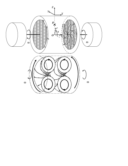
Figure 1: Top: experimental setup. The flow is produced in a cylindrical container by two counter-rotating propellers driven by two independent motors. (r, $\theta,z$) are the usual cylindrical coordinates. P represents the point where the magnetic field probe is located inside the VKS apparatus. (X, Y, Z) are the cartesian coordinates corresponding to the probe measurement axes. Bottom: schematic drawing of the von Kármán flow showing the mean toroidal and poloidal flows.

The experimental setup shown in figure 1 is a half-scale model of the sodium VKS experiment Bou02 . It consists of a cylindrical container of internal radius $R_{c}=10$ cm and height $H_{c}=30$ cm, filled with water. The system is driven by two counter-rotating co-axial disks of radius $R_{d}$, with their inner faces a distance $H_{d}=18$ cm apart. Different disks have been used: smooth or rough disks, disks with straight or curved blades with different heights. In the following, we report results concerning two different propellers: Propeller TM28 (resp. TM60) has a 180 mm diameter (resp. 185 mm), 8 blades (resp. 16) of 2 cm height. The blades of TM60 have a curvature slightly larger than those of TM28. Both propellers rotate as shown in figure 1. The propellers presently used in the VKS experiment are of the TM60 type. Baffles of different width and length can be introduced on the internal wall of the cylinder in order to change the ratio of axial to azimuthal components of the velocity field.

Two 2 kW motors are used to drive the disks in opposite directions at an adjustable frequency $f$ in the range 0-25 Hz. The measurements reported here have been performed in the range 0-10 Hz. A kinematic Reynolds number based on the driving is defined as: $Re=2\pi fR_{c}^{2}/\nu$, where $\nu$ is the kinematic viscosity of water.

Global measurements such as torque or power and pressure measurements have been performed in order to characterize the turbulence. The results will be reported in details elsewhere and show results typical of fully turbulent flows. In the following, we focus on the velocity measurements which are used in the numerical study.

2.2 Velocity fields

2.2.1 Measurement of the velocity field

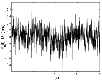
Figure 2: (a) Temporal evolution of the fluctuating part of the azimuthal velocity of TM60 propeller recorded using Laser Doppler Velocimetry at $r=60$ mm, $z=65$ mm for $f=2$ Hz. The value of the mean azimuthal velocity is $U_{\theta}=0.42\ {\rm ms}^{-1}$. (b) Probability density function for the same signal: data ($+$) and gaussian fit (solid line).

Velocity fields have been obtained via laser Doppler velocimetry (LDV) using a DANTEC system. The axial and azimuthal velocities $V_{z}$ and $V_{\theta}$ have been measured as functions of $r$, $z$ and time. At the rotation rates used in the experiment, the flow is highly turbulent: $Re\simeq 6.10^{5}$ for $f=10$ Hz. Figure 2 shows the temporal evolution of the local velocity at a given point: velocity fluctuations appear to be of the order of magnitude of the mean velocity, and have a quasi-gaussian distribution. In fact, the amplitude of the fluctuations as well as the shape of their probability density function strongly depend on the position inside the flow. The amplitude is particularly high in the plane between the two recirculation cells, where the strong toroidal shear maintains a vigorous mixing layer. More quantitatively, the turbulence intensity defined as $K_{V}=V_{rms}/U_{rim}$, where $V_{rms}$ is the order of magnitude of the standard deviation of the velocity throughout the flow and $U_{rim}$ is the rim velocity of the disks, is roughly 40 %.

As a consequence, the velocity can be seen as a mean flow plus a turbulent part: $\vec{V}=\vec{U}+\vec{u}$. In the following, $\vec{U}$ denotes a time averaged flow, and $\vec{V}$ a velocity field that depends on time.

The LDV facility gives only the axial and azimuthal instantaneous velocity, whereas the induction equation asks for the three time-averaged components. The missing mean radial velocity is derived as follows. Note that, although $\vec{U}$ is not a solution of the Navier Stokes equations, it is a solenoidal vector field, and it can always be decomposed into toroidal and poloidal components:

$$\vec{U}(r,\theta,z)=\nabla\times(T\hat{z})+\nabla\times\nabla\times(P\hat{z})=\vec{U}_{tor}+\vec{U}_{pol}$$

where $\hat{z}$ is the unitary vector in the axial direction. Assuming now that $\vec{U}$ is axisymmetric (it is not strictly the case when four axial baffles are used), its toroidal component reduces to the azimuthal velocity, while its poloidal component is found to lie in the meridian planes

$$\vec{U}_{tor}(r,z) = U_{\theta}(r,z)\ \hat{\theta}$$

$$\vec{U}_{pol}(r,z) = \nabla\times(\partial_{r}P\ \hat{\theta})=\hat{\theta}\times(1/r\,\nabla\psi(r,z))$$

$$\vec{U}_{pol}(r,z) = U_{r}(r,z)\ \hat{r}+U_{z}(r,z)\ \hat{z}$$

where $\hat{r}$ and $\hat{\theta}$ are the unitary vectors in the radial and azimuthal directions. The poloidal scalar P is thus replaced by the flux function $\psi(r,z)$, such that

$$U_{r}(r,z) = 1/r\,\partial_{z}\psi$$

$$U_{z}(r,z) = -1/r\,\partial_{r}\psi$$

so that finally $U_{r}$ can be derived from the experimental knowledge of the field $U_{z}(r,z)$.

The velocity field input in the kinematic dynamo code is obtained in the following way: (i) The time averaged $U_{\theta}$ and $U_{z}$ are measured on a $11\times 15$ grid in the plane $\theta=0$ of figure 1, outside the region swept by the propeller blades. (ii) In the region swept by the propeller blades, we interpolate lines $z=0,\ 16,\ 17$, making the hypothesis that $U_{z}$ depends linearly in $z$ and $U_{\theta}$ does not depend on $z$. (iii) From the obtained $11\times 18$ $U_{z}$ velocity field, we compute the flux function $\psi$ by a radial integration between the axis and the container wall. (iv) $\psi$ and $U_{\theta}$ are smoothed using a standard $3\times 3$ convolution filter. (v) $\psi$ and $U_{\theta}$ are then periodized in the z-direction in order to eliminate Gibbs phenomenon in the code. Axial periodicity is obtained by completing the measured flow by its symmetric with respect to the plane of any of the container tops (as translation of length $L$ is obtained by the product of two reflections by parallel planes distant of $L/2$). (vi) $\psi$ and $U_{\theta}$ are then interpolated linearly to the final $48(z)\times 51(r)$ simulation resolution. (vii) $U_{r}$ is then derived from $\psi$.

Note that the periodization of the flow implies that the toroidal flow can be decomposed on $n^{\prime}$ odd modes, while the poloidal flow can be decomposed on $n^{\prime}$ even modes. The magnetic eigenmodes depend on these symmetry properties of the simulated flow.

2.2.2 Characterization of the velocity field

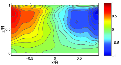
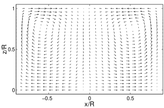
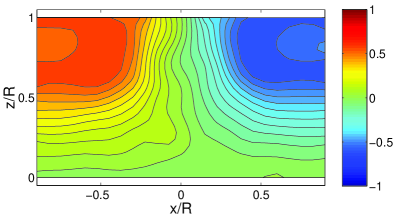
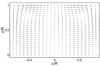
Figure 3: Mean velocity field. TM28 propeller velocity field: (a) toroidal and (b) poloidal component in a meridional plane. TM60 propeller velocity field: (c) toroidal and (d) poloidal component.

Different driving devices have been tested and each configuration gives a different velocity field. Figure 3 shows the toroidal and poloidal components of the mean velocity field for the propellers TM28 and TM60 without baffles. The two velocity fields appear to be similar, but we will see later that TM28 and TM60 display quite different dynamo properties.

In table 1, the main characteristics of these velocity fields are summarized. The spatial mean speed in the measured volume, including blades, is defined as:

$$U_{mean}={1\over V}\int_{V}|\vec{U}(r,z)|dV$$

and the efficiency $E_{f}$ of the propeller as: $E_{f}=U_{\rm max}/2\pi R_{c}f$. $U_{max}$ represents the maximum value of the speed in the measured volume. Typically, $U_{max}\leq U_{\rm rim}$.

As can be seen in table 1, the efficiency of propeller TM28 is 25% larger than that of propeller TM60. Note that the efficiency of a straight-blade propeller is closer to unity. As could be expected from the curvature difference, the poloidal-to-toroidal ratio of propeller TM60 is larger than that of propeller TM28. This gain in poloidal-to-toroidal ratio is however offset by the loss in efficiency, so that the poloidal flow of TM60 is smaller than that of TM28.

The largest values of the velocity can be found close to the propeller rims. This is true for both the poloidal and the toroidal velocities, regardless of the propeller used.

For a typical pair of propellers, we have performed velocity field measurements at different rotation rates, 2.5, 5 and 7.5 Hz. At every location inside the flow, the measured velocity is proportional to the rotation rate. This result could be expected from standard hydrodynamics arguments. As a further consequence, changing the magnetic Reynolds number by a simple scaling of the flow seems reasonable. This property will be used in the numerical code.

3 Numerical resolution of the induction equation

3.1 Scope of the numerical approach

The numerical dynamo problem asks for the resolution of two coupled sets of equations, one for the velocity field and one for the induction equation. In the context of experimental dynamos using liquid sodium, at $R_{\rm m}=100$, the kinetic Reynolds number of the flow will reach $10^{7}$, which is far out of range of any direct numerical simulation. This is why scaled down water experiments are needed to measure the mean flow velocity field, to estimate the mechanical torque necessary to drive the flow as well as the dissipated power. Although the chaotic properties of the flow may play an essential role for the dynamo action in specific configurations, there is presently no way to determine the time dependent turbulent velocity field.

An alternative to the fully nonlinear dynamo solution is the ”kinematic” approach, where the flow is considered as given in the evolution equation of the magnetic field. Starting with a faint seed field, this approximation is valid as long as the magnetic force field remains small. A better contact with experiments may be obtained if the time dependent solutions are obtained, instead of choosing to solve an eigenvalue problem. In this case, for flows at magnetic Reynolds numbers below the critical value, one may study the magnetic response to external magnetic fields, possibly time-dependent, in order to get an experimental estimate of the critical $R_{\rm m}$. Finally, note that while the nonlinear simulations need a challenging amount of numerical ressources, the parameter space may be explored more rapidly and thoroughly using the kinematic solution. When following an optimization procedure, this is a meaningful practical point. A typical example is given below by the variation of the thickness of an high conductivity blanket, which allows to reduce the critical $R_{\rm m}$.

3.2 The kinematic dynamo code

As explained above, we consider that the velocity field is known in a cylindrical container of radius $R_{c}$. Moreover we assume that the conductivity $\sigma$ of the fluid inside the cylinder is uniform, the external medium is insulating and that the magnetic permeability is uniform in all space.

The induction equation is adimensionalized using the cylinder radius as length unit and the ohmic diffusion time $t_{d}=\mu_{0}\sigma R_{c}^{2}$ as time unit. The induction equation reads then

$$\partial_{t}\vec{B}=R_{\rm m}\nabla\times\left(\vec{U}\times\vec{B}\right)+\nabla^{2}\vec{B}.$$

Notice that the initial magnetic field must satisfy

$$\nabla.\vec{B}=0.$$

Boundary conditions are implemented as follows. The magnetic field must be continuous at the cylinder boundary, from Maxwell equations. The external field is curl-free and derives from an harmonic scalar potential, which is completely defined by, say, its gradient normal to the cylinder, i.e. the magnetic field orthogonal to the boundary. For a given conducting volume, the numerical determination of the external harmonic potential from its gradient at the surface boundary may involve substantial numerical resources, and this is in particular the case for a cylinder of finite length. We have chosen here to avoid this problem by solving the induction equation for axially periodic flows, where there is an analytical solution for the external potential, as is also the case for the spherical geometry.

The magnetic field has thus the following representation,

$$\vec{B}(r,\varphi,z,t)=\sum_{n,m}\vec{B}^{n,m}(r,t)\exp\left[i(m\theta+nz)\right],$$

where the z coordinate ($0\leq z\leq 2\pi$) has been scaled with the axial period and the integers n et m characterize the axial and azimuthal modes. The spatial scheme is pseudospectral in the azimuthal and axial directions, and uses compact finite differences in the radial direction.

Let us summarize now the formal organisation of the temporal scheme. Suppose that at time $t^{i}$ the internal magnetic field ${\bf b}({\bf r},t^{i})$ is known: from the normal component of the surface field ${\bf b}_{\perp}({\bf S},t^{i})$, where ${\bf S}$ is a point on the surface $r=1$, one may get the external potential for the next time step, ${\phi({\bf r},t^{i+1})(r>1)}$ and the corresponding tangential magnetic field is then obtained by differentiation ${\bf b}_{\parallel}({\bf S},t^{i+1})=\vec{\nabla}_{\parallel}\phi({\bf S},t^{i+1})$. These two components are the two boundary conditions used for the integration of the dynamo equation within the cylinder, which gives finally the internal field ${\bf b}({\bf r},t^{i+1}),(r<1)$ at time step $i+1$. The time scheme is second order Adams-Bashforth for the non linear terms, while the purely multiplicative parts of the diffusive terms are integrated exactly. The integration variables are the three components of the magnetic field, and this allows to follow the growth of the divergence of the magnetic field, whose solenoidal property is not preserved under this algorithm (the discretized expression of div curl is not zero). To keep the divergence small, the numerical solution is projected, every 40 steps, say, on a divergenceless field. Other features of the code have been described elsewhere Leo98 .

Comparisons with a finite cylinder dynamo code (performed by F. Stefani, RFZ, Dresden) have not shown significant differences for the critical $R_{\rm m}$ with respect to the simpler periodic solution having an identical aspect ratio, at least for a few flow configurations which have been tested.

4 Results

Dynamo action may take place if the energy generation by stretching dominates the ohmic dissipation. This is measured in a loose way by the magnitude of the magnetic Reynolds number $R_{\rm m}$ which appears after adimensionalization of the equation with the maximal flow speed $U$ and a container typical scale $L$. This necessary condition is useless to select flows which are indeed efficient dynamos, i.e. flows with small critical magnetic Reynolds numbers. Numerical kinematic dynamos are generally obtained from successive attempts with flows given by a few velocity components selected for analytical simplicity (see e.g. Dud89 ). In this section, we present numerical results obtained with the mean experimental velocity fields presented above.

As explained in paragraph 4.2.2, these velocity fields present a slight experimental disymmetry, which has a small influence on the obtained results. We have thus prefered to first present the results with a symmetrized velocity field and then to study the influence of this additional parameter. These results first concern threshold determination and the influence of different parameters on it. We then give a description of the spatio-temporal characteristics of the self-excited magnetic field mode. In order to compare the numerical results to available experimental data, we finally study the response of the system to an external magnetic field for $R_{\rm m}$ below the dynamo threshold.

4.1 Threshold determination

For a given experimental configuration, the mean velocity field shape is fixed, and cannot be varied. As indicated in Section 2, varying the propellers rotation rate, we are only modifying $R_{\rm m}$ in the induction equation, but not the field shape. The effect of turbulence is not taken into account.

For each experimental velocity field, we have performed a series of numerical runs with the kinematic dynamo code, at different $Rm$, and checked the energy evolution of each mode $m,n$, defined as follows:

$$E^{n,m}(t)=\int_{0}^{1}|{\vec{B}}^{n,m}(r,t)|^{2}rdr\sim e^{\sigma_{n,m}t}$$

Note that the different azimuthal $m$-modes are decoupled, since only axisymmetric flows are considered. Self excitation is achieved when the energy $E^{n,m}$ grows in at least a single mode without external magnetic excitation that is if $\sigma_{n,m}>0$ for at least a pair ${n,m}$. If $\sigma_{n,m}<0\,\,\,\forall n,m$, ohmic diffusion dominates.

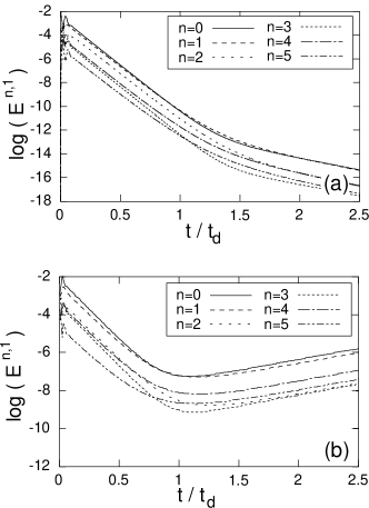
Figure 4: Temporal evolution of the energy of modes $m=1;n=0,..,5$ for TM28 propeller. (a) $R_{\rm m}=100<R_{\rm m}^{c}$ (b) $R_{\rm m}=140>R_{\rm m}^{c}$. The time unit corresponds to the ohmic diffusion time. Two different regions can be distinguished: for $t/t_{d}\leq 1$, relaxation of the fast stable modes; for $t/t_{d}\geq 1$, relaxation of the slow stable modes (a), or growth of the unstable modes (b). Note that in both cases the evolution is exponential with a growth rate $\sigma<0$ (a) and $\sigma>0$ (b).

Figure 4 displays the evolution in time of $E^{n,m}$ for $m=1$ and $n=0,...,5$ for the velocity field labelled TM28 under and above threshold. The initial condition is:

$$E^{n,m}(t)=\left\{\matrix{1.0&{\rm when\ }m=0,1,2,3;\,\,n=0&\cr 0.2&{\rm when\ }m=0,1,2,3;\,\,n=1,...,7\cr 0.0&{\rm in\ any\ other\ case}\cr}\right.$$

In both cases, a transient regime corresponding to the relaxation of the initial field is observed until $t\simeq t_{d}$. For $R_{\rm m}<R_{\rm m}^{c}$, the energy in all modes decreases in time, i.e. the growth rates are negative (figure 4a). For $R_{\rm m}\geq R_{\rm m}^{c}$, the energy of some modes begins to grow (figure 4b). The critical magnetic Reynolds number $R_{\rm m}^{c}$ is defined as the value for which at least one growth rate is greater or equal to zero. For the velocity fields tested, self-excitation always appears through the $m=1$ mode. Remember that, as the flow is axisymmetric, an axisymmetric ($m=0$) self-excited magnetic field is forbidden by anti-dynamo theorems Mof78 .

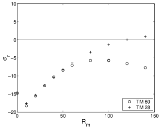
Figure 5: Energy growth rates $\sigma_{r}$ for the most unstable mode ($n=1$ and $m=1$) as a function of $R_{\rm m}$. Crosses (resp. circles) correspond to the symmetrized velocity field of TM28 (resp. TM60) propeller. The TM28 propeller gives rise to dynamo action for $R_{\rm m}\simeq 120$ whereas TM60 does not.

In the following, for numerical efficiency, a different initial condition has been used, namely the (solenoidal) eigenmode of the vector laplacian which is closest in shape to the most unstable mode of the induction equation (cf. section 4.2). The energy is thus initially distributed on the $m=1$, $n$ odd Fourier modes. This leads to the near elimination of the transient regimes of figure 4. The variation of the maximal growth rate is presented in figure 5 as a fonction of $R_{\rm m}$ for the two velocity fields of figure 3. The velocity field corresponding to propeller TM28 exhibits a growth rate that crosses the zero line for $R_{\rm m}^{c}\simeq 120$ and gives rise to dynamo action. On the contrary, for the propeller TM60, the growth rate remains negative: it saturates for $R_{\rm m}\simeq 80$, and then decreases again. This latter result corresponds to a non-dynamo velocity field. Performing simulations for $R_{\rm m}$ up to 300, we have observed that the growth rate for TM28 (resp. TM60) keeps increasing (resp. decreasing). At those large values of $R_{\rm m}$, simulation results are not accurate enough to obtain a precise scaling of $\sigma(R_{\rm m})$. A linear scaling of $\sigma$ with $R_{\rm m}$ would indicate a saturation of $\sigma$, if expressed with the convective time unit $t_{d}/R_{\rm m}$.

The existence and the exact value of $R_{\rm m}^{c}$ strongly depends on the characteristics of the velocity field and on the boundary conditions. To investigate this dependence, we have modified different parameters. First, the velocity fields have been modified in a controled manner in the numerical simulations, changing the ratio between the poloidal and toroidal velocity components. We have then investigated the effect of a conducting layer (with various thicknesses) surrounding the flow container.

4.1.1 Ratio between the poloidal and toroidal velocity components

Because of the flow axisymmetry (see section 2.2), we can keep the solenoidal character of the flow, when changing the ratio $\Gamma=\overline{|{\vec{U}}_{pol}|}\,/\,\overline{|{\vec{U}}_{tor}|}$ where

$$\overline{|{\vec{U}}_{pol,tor}|}=\int_{V}|{\vec{U}}_{pol,tor}|\,\,r\,dr\,dz$$

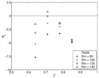
Figure 6: Energy growth rates $\sigma_{r}$ for the mode $n=1$ and $m=1$ as a function of the mean poloidal-to-toroidal ratio $\Gamma=U_{pol}/U_{tor}$ for various $R_{\rm m}$. The plotted data correspond to the symmetrized TM28 velocity field which as a natural ratio $\Gamma=0.71$.

and look at the effect of $\Gamma$ on the critical magnetic Reynolds number. The $\Gamma$ parameter strongly affects the growth rates, as can be observed in figure 6 for TM28 propeller: a negative growth rate can become positive and vice-versa. Most of the studied velocity fields present a maximum growth rate for $\Gamma\simeq 0.75$. This result is recovered for both dynamo and non-dynamo velocity fields such as the TM60. The optimal value $\Gamma_{\rm opt}$ corresponds nearly to the experimental value for the TM28 propeller ($\Gamma_{\rm exp}=0.71$), while it is different in the case of TM60 propeller ($\Gamma_{\rm exp}=0.82$).

In a von Kármán flow, this parameter can be adjusted within certain limits in various ways e.g. by changing the diameter of the disc or the curvature of the blades (cf. Table 1) or by fitting baffles located on the cylinder wall. Four baffles can be placed parallel to the cylinder axis at azimuthal intervals of $\pi/2$. These baffles break the axisymmetry of the problem, making it necessary to measure the full three-dimensional velocity field. This also imposes a higher resolution in the azimuthal direction in the code, making simulations more time-consuming. We have not performed systematic exploration of these effects, and will not present here the corresponding results.

Figure 6 also reveals a difference in the variation of the growth rate with $R_{\rm m}$ depending on the value of $\Gamma$. For $\Gamma\simeq 0.5$, $\sigma$ varies quasi-linearly with $R_{\rm m}$, while for $\Gamma\simeq 1$, $\sigma$ seems independent of $R_{\rm m}$.

4.1.2 Conducting layer

It is empirically known that a stagnant layer of conducting material surrounding some fluid dynamos may reduce the critical magnetic Reynolds number. In the case of the Riga experiment Gai00 , this has also been numerically verified by Stefani et al. GaiXX . The example of the Ponomarenko dynamo has been systematically examined in Kai99 , varying the thickness of the static conducting layer, and the authors show that there is an optimal thickness leading to a lowest critical Rm. A similar configuration is available in the VKS experiment Bou02 with a copper wall put inside the stainless steel cylindrical container.

As indicated in Section 3, the numerical simulations are performed with a conductivity which is uniform inside a cylinder and insulating boundary conditions. A static conductive shell of arbitrary thickness may thus be easily introduced only if it has the same conductivity as the fluid. If the flow lies within a radius $R_{c}$, the stationary shell goes from $r=R_{c}$, to $r=R_{ext}$, and we can use as control parameter the relative width $W=(R_{ext}/R_{c})-1$. Note that we have chosen to present the numerical results with the magnetic Reynolds defined with the radius $R_{c}$.

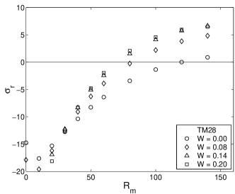
Figure 7: Conducting layer effect: Maximal growth rate $\sigma_{r}$ as a function of $R_{\rm m}$ for different layer thicknesses $W=(R_{ext}/R_{c})-1$; symmetrized velocity field of propeller (a) TM28 and (b) TM60.

Figure 7 displays the effect of a conductive layer for propeller TM28 and for propeller TM60. The first effect concerns the growth rates that increase with $W$, until they saturate for $W=W_{s}\simeq 0.2$. For propeller TM28, the threshold $R_{\rm m}^{c}$ decreases from 120 for $W=0$ to 70 for $W=0.2$ (cf. Figure 7a). The second important effect concerns the fact that the presence of a conducting layer can actually change a non-dynamo velocity field into a dynamo velocity field: $R_{\rm m}^{c}=60$ for propeller TM60 and $W=0.2$, which is actually smaller than the threshold for TM28 (cf. Figure 7b).

4.2 Description of the self-excited magnetic field

In the following, we describe the self-excited magnetic field numerically observed with propeller TM28. This field appears to have a very complicated spatial structure and its temporal behaviour depends on the symmetry of the velocity field.

4.2.1 Spatial characteristics

It is well known that a smooth velocity field with a few spatial modes gives generally rise to magnetic eigenmodes with a broad band spectrum, and complex spatial configuration, and we have verified that it is indeed the case for the flows we have used. Although small variations of the flow may induce large changes in the value of the critical magnetic Reynolds number, we have observed that the overall neutral mode topology is not much altered, so that we choose to present a single example.

As noted above, in an axisymmetric flow, the different azimuthal modes evolve independently and close to the critical $R_{\rm m}$, it is the mode m=1 which has the largest growth rate (recall that m=0 modes always decay). The magnetic axial modes (n) are coupled by the kinetic ones, so that the axial spectrum is continuous from n=1 to the ohmic dissipation wavenumber.

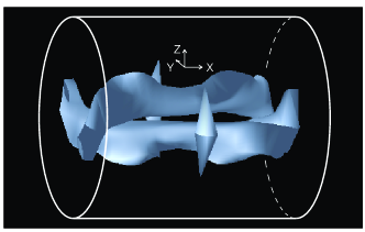
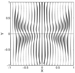
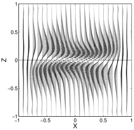
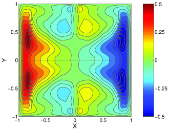
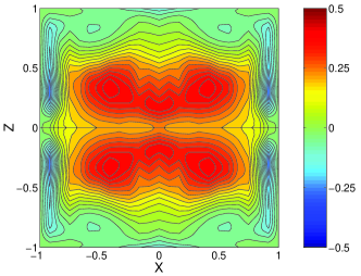
Figure 8: Self-excited magnetic field of propeller TM28 for $R_{\rm m}=140$. (a) Isosurface of the magnetic energy at 50 % of the maximum value in the simulation volume. Poloidal component of the magnetic field in (X,Y) plane (b) and (X,Z) plane (c). (d) Z component of the magnetic field in (X,Y) plane; red (resp. blue) corresponds to vectors pointing out of (resp. into) the plane. (e) Y component in the (X,Z) plane; blue (resp. red) corresponds to vectors pointing out of (resp. into) the plane.

Figure 8 represents a typical example of the growing mode structure, obtained for $R_{\rm m}=140$, with the TM28 velocity field, in which symmetry has been artificially imposed. Figure 8a shows the zones where the magnetic field intensity is higher than 50% of its maximum value. The magnetic field appears to be strong principally in two banana-shaped regions, located on either sides of the cylinder axis. Figure 8b shows the poloidal component of the magnetic field in the plane XOY of figure 1. In that plane, the magnetic field is roughly dipolar, oriented perpendicularly to the cylinder axis. This corresponds to an m=1 angular dependency. On either sides of the dipole, we can see in figure 8b the ends of the banana-shaped regions of figure 8a. Figure 8c shows the poloidal component of the magnetic field in the plane XOZ of figure 1. The magnetic field has a large amplitude in a significant portion of the regions in this plane. The magnetic field there is axial, and has the expected m=1 angular dependency. Figure 8d and 8e show the components of the magnetic field normal to the XOY and XOZ planes, respectively.

From all these figures, we can gather that the magnetic field of the most unstable mode is roughly a dipole, oriented perpendicularly to the cylinder axis, in the plane of figure 8b, normally into the plane of figure 8e. Around this dipole, a group of magnetic field lines comes upwards from the bottom left-hand of figure 8d, follows the arrows in the top half of figure 8c, and then goes downwards at the top right-hand of figure 8d. The m=1 angular dependency implies that another group of magnetic field lines goes in the converse way, going into the bottom right-hand of figure 8d, to the left in figure 8c, and then upwards in the top left-hand corner of figure 8d.

The electric current distribution associated to this magnetic field structure is also quite similar in all situations. The electric currents concentrate in an elongated cylindrical region, located between the two regions of large magnetic field amplitude. Inside this region, the currents point perpendicularly to the axis, in the same direction as the magnetic field dipole.

4.2.2 Temporal characteristics

We have observed that the growth rate of the most unstable mode can have an imaginary part. The corresponding frequency is associated with a rotation of the magnetic field around the cylinder axis. This frequency is very sensitive to the level of symmetry of the velocity field. In fact, for a very symmetric velocity field such as the TM28, the neutral mode is nearly stationary, whereas for strongly dissymetric ones the growth rate can have a much larger imaginary part.

In order to study this dependency, we have separated the TM28 velocity field into two parts $\vec{U}_{even}$ and $\vec{U}_{odd}$ defined by their parities with respect to the rotation around the OP axis of figure 1.

In the case of TM28, we have checked that the velocity field odd component $\vec{U}_{odd}$, being mainly due to experimental imperfections, is small compared to the even component $\vec{U}_{even}$: $\vec{U}_{odd}\simeq 0.1\vec{U}_{even}$. We have then performed simulations of the composite flow $\vec{U}=\vec{U}_{even}+\varepsilon\vec{U}_{odd}$ for various values of $\epsilon$, while keeping the $R_{\rm m}$ based on $\vec{U}_{even}$ at a constant value of 160. The value $\varepsilon=1$ corresponds to the experimental TM 28 flow.

The dependency of the imaginary part of the growth rate on $\epsilon$ is shown in figure 9. We can see that this dependency is very nearly linear, and that $\epsilon=0$, which means a perfectly symmetric flow, is associated with a stationary magnetic field neutral mode. This behaviour is observed with other velocity fields and seems to be robust in von Kármán type flows. Note that the real part of the growth rate presents a small variation with $\varepsilon$.

4.3 Magnetic induction by an external field

In the following, we want to address the following question: is it possible to use the magnetic response of the experimental flow below $R_{\rm m}^{c}$ to an external magnetic field to predict the value of $R_{\rm m}^{c}$?

The kinematic code and the experimental velocity fields can be used to obtain the response of the system to an external magnetic field $\vec{B}_{0}$ and to perform a comparison with sodium experiments. We have checked the response to two different external magnetic fields: an axial field, parallel to the axis of rotation (along $X$) or a transverse field, orthogonal to the rotation axis (along $Y$).

In both cases, we have performed global and local measurements. We have first determined the decay times of the energy of each mode, and the saturation value of the magnetic field induced inside the numerical box. In order to make a quantitative comparison with the results obtained in the VKS experiment, we have then studied the local components of the induced magnetic field at a particular point in the experiment (point P of figure 1).

4.3.1 Magnetic energy measurements

Each numerical run is performed for a given velocity field as follows. The initial condition corresponds to no magnetic field inside the cylinder. At $t=0$, an external magnetic field is switched on and we let the system evolve in time. This transverse field is directed along Y. It is sinusoidal with a $n=1$ axial dependency and its maximal amplitude is 1. We have chosen this external field structure because a uniform ($n=0$) transverse field, which would have been easier to implement, as well as closer to the experimental setup, is orthogonal to the growing magnetic field eigenmodes we have observed. This feature is specific to the axially periodic induction code.

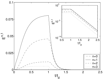
Figure 10: Response to an external transverse magnetic field, varying sinusoidaly along the axis, of the symmetrized TM28 velocity field: temporal evolution of the energy for the modes $m=1;n=0,...,3$ when $R_{\rm m}=40<R_{\rm m}^{c}$. The external field is applied for $0<t<1$. It has an n=1 axial dependency, and has a maximal amplitude of 1.

For small $t$, the external field enters the cylinder, until it approaches asymptotically a stationary saturated state of energy $E_{\rm sat}$ (see figure 10, for $t<1$, $m=1,n=0-3$):

$$E(t)=E_{\rm sat}\left(1-\exp(-t/\tau_{\rm sat})\right)$$

Where $\tau_{\rm sat}$ is the saturation characteristic time. This time diverges at the dynamo threshold of the TM28 system. After the stationary state has been reached, the external field is disconnected, and we look at the magnetic energy decay time (see figure 10, for $t>1$):

$$E(t)=E_{\rm sat}\exp(-t/\tau_{\rm decay})$$

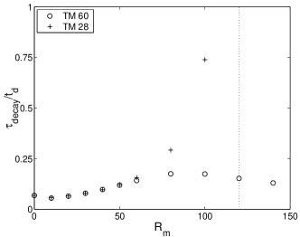
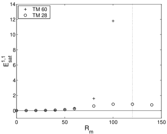
Figure 11: variation of (a) the energy decay time $\tau_{decay}$ and (b) the saturation value of the magnetic energy $E^{n=1,m=1}_{\rm sat}$ as a function of $R_{\rm m}$ for an external transverse magnetic field . Crosses: TM28 propeller; circles: TM60 propeller. Note that both the decay time and the energy diverge when TM28 approaches threshold (dotted line).

Figure 11 shows the variation of the decay characteristic times $\tau_{\rm decay}$ and the saturation value of the magnetic energy with $R_{\rm m}$. Both quantities diverge for TM28 propeller near $R_{\rm m}^{c}=120$ while they saturate near $R_{\rm m}=80$ and then decrease for TM60 propeller. We found that, below $R_{\rm m}=60$, theses features do not appear in practice to be good candidates to discriminate between a dynamo and a non dynamo velocity field.

4.3.2 Local magnetic field measurements

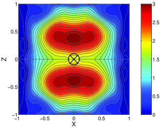
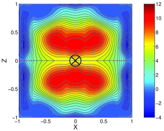
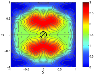
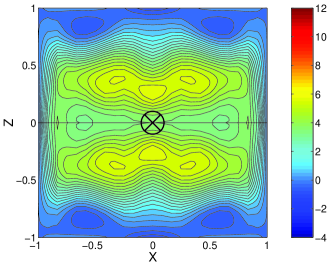
Figure 12: Representation in the plane (X,Z) of the $B_{Y}$ component of the magnetic field in the presence of an external transverse magnetic field varying sinusoidally along the axis (reprented schematically by the central cross). Propeller TM28: (a)$R_{\rm m}=50$ and (b) $R_{\rm m}=80$. Propeller TM60: (c)$R_{\rm m}=50$ and (d) $R_{\rm m}=80$. blue (resp. red) corresponds to vectors pointing out of (resp. into) the plane

The spatial structure of the magnetic field in the presence of the transverse magnetic field is represented in the plane (XOZ) in figure 12. For $R_{\rm m}=50$, the structures of the two magnetic fields look similar, and the intensity of the induced field appears to be slightly larger for TM28 than for TM60 velocity field. The difference between the two fields increases with $R_{\rm m}$. For $R_{\rm m}=80$, the amplitude of the magnetic field corresponding to TM28 appears to be twice that corresponding to TM60. Spatially, a spreading of the magnetic field is observed in the case of TM60, while strong gradients along $X$ can be evidenced for TM28, with an inversion of the magnetic field close to the disks.

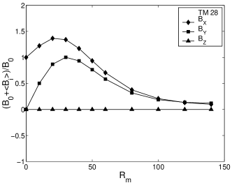
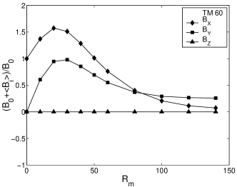
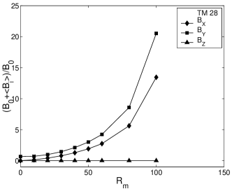
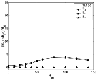
Figure 13: Asymptotic values of three components of the magnetic field at position P as a function of $R_{\rm m}$. Diamonds, squares and disks respectively refer to $B_{X}$, $B_{Y}$ and $B_{Z}$. Response of the TM28 (a) and the TM60 (b) symmetrized velocity field, to an axial magnetic field. Response of the TM28 (c) and the TM60 (d) velocity field, to a transverse magnetic field varying sinusoidaly along the axis.

We have studied the magnetic field induced at the point P of figure 1 by an external axial or transverse field in the symmetrized TM28 and TM60 flows. This point corresponds to the main measurement location in the VKS experiment Bou02 . In figure 13, we have plotted the variation of the three components of the magnetic field as a function of $R_{\rm m}$. We can see that in all cases the Z-component of the magnetic field is equal to zero. We have checked that this is a consequence of the symmetry of the flow Pet02 .

In the case of an axial external magnetic field (figure 13 a and b), the magnetic field components increase, then saturate for $R_{\rm m}\simeq 30$ and eventually decrease to zero for both propellers. This behaviour is akin to the expulsion of poloidal magnetic field expected in poloidal circulation Mof78 in spite of the existence of a toroidal flow.

For a transverse field, figures 13 c and d show that, for the TM28 velocity field which gives rise to dynamo action, the amplitude of the induced magnetic field components diverges as one approaches the threshold. Conversely, in the case of the TM60 velocity field, which does not lead to dynamo instability, the amplitudes remain bounded. Indeed we can see that the magnetic field components increase for an interval in $R_{\rm m}$, then saturate for $R_{\rm m}\simeq 80$, and eventually start to decrease. Inspection of the growth rates shows that the magnetic field growth rate, while remaining negative, has a maximum for the same value of $R_{\rm m}$ (cf. figure 5).

5 Discussion

5.1 Status of the von Kármán flow with respect to other dynamo flows

Starting from an experimentally produced flow, we have shown that it may produce kinematic dynamo action above some critical $R_{\rm m}^{c}$, which could no be reached up to now in the VKS experiment due to insufficient driving power. It is instructive to examine how these results compare with other known laminar axisymmetric dynamos, on the one hand, and available experimental dynamos, on the other hand.

Most numerical dynamo flows in a finite volume are produced in a spherical container, since the magnetic transmission conditions at the conducting-insulating interface are easier to implement. For example, the Von Kármán flow has the same symmetry properties as the spherical configuration denoted $s2t2$ by  Dud89 , which has a $R_{\rm m}^{c}=54$ with the particular radial function chosen by these authors. The same spherical $s2t2$ configuration has been chosen for the Maryland  Pef00 ; Pef01 and the Madison experiment  For01 , which use two counter-rotating coaxial turbines set in motion by two motors to drive the flow. The Maryland experiment uses a 30 cm diameter sphere and has not produced dynamo action. The Madison installation is based on a one meter diameter sphere, where the velocity field could be measured using water as a fluid in a first step and the driving configuration has been optimized with the help of a kinematic dynamo code to get $R_{\rm m}^{c}=100$. The liquid sodium installation is almost ready to be set in operation.

The two existing experimental dynamos in Riga and in Karlsruhe were based on flows of previous theoretical interest as occurrence of dynamo action in these flows may be proved analytically. They are not axisymmetric but involve helicoidal streamlines winding around unbounded cylinders, the conducting fluid filling all space. In the experimental devices, the flow is constrained by cylindrical pipes of finite length, with guiding blades (Riga) or internal helicoidal walls (Karlsruhe) and occupies obviously a finite volume container. In both cases, the design studies have concentrated on the search of a lower $R_{\rm m}^{c}$. Although the two configurations are very different, they lead to comparable critical magnetic Reynolds numbers based on a flow maximal speed V and a typical scale for the conducting fluid :

• Riga experiment : $R_{\rm m}^{c}\simeq 61$, with $V=15$ m/s, $L=0.4$ m ($L=$ external cylinder radius)

• Karlsruhe experiment : $R_{\rm m}^{c}\simeq 36$, with $V=4$ m/s, $L=0.9$ m ($L=$ container radius)

Recall from Section 4 that $R_{\rm m}^{c}$ around $60$ (resp. $70$) has also been found for the TM60 (resp. TM28) flow with the adjunction of a conducting shell W= 0.2, so that the lowest $R_{\rm m}^{c}$ are indeed comparable for these cylindrical dynamos. There remains however a fundamental difference between these MHD flows at large $R_{\rm m}$: the turbulence level varies from a few percent for the flows with internal walls to 40% for the VKS configuration, where the flow is not guided. In the latter case, it has been verified that the power scales as $R_{\rm m}^{3}$ Bou02 , in agreement with dimensional analysis arguments. To reach the numerically predicted $R_{\rm m}^{c}$, one has thus to overcome a power challenge: this is the price to pay to drive a flow without the constraint of internal walls, such that its non linear saturation regime could have a link with those observed in natural dynamos.

5.2 Threshold: comparison with VKS experiment

The kinematic dynamo simulations based on experimental mean velocity fields of von Kármán flows exhibit the existence of self-excitation in some range of parameters that can be compared to experimental results of the VKS experiment. The minimum threshold value $R_{\rm m}^{c}\simeq 60$ is found for the TM60 propeller, with a 20% layer of liquid at rest. These numerical results correspond to a 4 cm sodium layer of conductivity $\sigma_{\rm Na}$ at rest, whereas the experiment is performed with a 1 cm thick copper boundary of conductivity $\sigma_{\rm Cu}\simeq 4\sigma_{\rm Na}$. Note that as far as the ohmic diffusion time is concerned, we expect 4 cm of sodium to correspond to 2 cm of copper.

Using the following definition for the experimental magnetic Reynolds number:

$$R_{\rm m}=\mu_{0}\sigma E_{f}R_{c}^{2}2\pi f$$ (1)

$R_{\rm m}^{c}=60$ would correspond to a critical rotation frequency $f^{c}=44$ Hz in the VKS experiment ($R_{c}=0.205$ m, TM60 propeller Bou02 ). This last value can be compared to the maximum frequency obtained in the sodium experiment $f=25$ Hz. As the flow is highly turbulent, the power needed to maintain the flow scales as Fri95 :

$$P=K_{P}\rho L^{2}U^{3}$$ (2)

where $K_{P}$ is a dimensionless factor that depends on the geometry of the container and of the shape of the propellers. We can write the magnetic Reynolds number as:

$$R_{m}=\mu_{0}\sigma E_{f}\left({PL\over K_{P}\rho}\right)^{1/3}.$$ (3)

Going from 25 to 44 Hz thus implies to increase the power or the scale of the experiment by a factor 5, that is $P=750$ kW or $R_{c}=1$ m.

In the case of the TM28 propeller, the minimum threshold value is $R_{\rm m}^{c}\simeq 70$ which corresponds to a critical $f^{c}=41$ Hz. This lower value of the critical frequency of rotation can be related to the efficiency of propeller TM28 that is superior to that of TM60. In fact, the important parameter of a flow configuration is given by the ratio $E_{f}/K_{p}^{1/3}$, and a minimum $R_{\rm m}^{c}$ does not necessary corresponds to the most easily achievable critical frequency.

5.3 Sensitivity to configuration parameters

5.3.1 Propellers

One aim of this work is to test the effect of various characteristics of the velocity fields on the existence and the value of the critical magnetic Reynolds number $R_{\rm m}^{c}$. One method would be to try different velocity fields that can be obtained from analytical expressions, or to modify continuously an experimental one. A continuous optimization could be performed in this way until the velocity field with the minimum $R_{\rm m}^{c}$ is obtained. However, in a real system with no guiding walls, it is a technological challenge to design a propeller able to reproduce the numerically optimized velocity field.

We have taken an experimental approach having in mind a possible sodium experiment. Consequently, we have not varied a configuration in a continuous manner but tried several driving configurations. Although the presented results concern only two different propellers, we have tested approximatively 30 other configurations. Various parameters have been varied: the height and curvature of the blades, the propeller diameter, and other characteristics. Nevertheless, the presented cases correspond to representative ones, and enlighten the fact that two very close velocity fields can have very different dynamo properties. The results do not reveal which characteristics a propeller must fullfill to produce dynamo action, but nevertheless some conclusions can be drawn.

The poloidal to toroidal ratio appears to be a crucial parameter to obtain a dynamo velocity field, as already known from other numerical studies, in various geometries. The condition $\Gamma\simeq 0.75$ (see figure 6) corresponds to a maximum growth rate for the explored velocity fields, but it is not a sufficient condition. No dynamo action has been observed with velocity fields with $\Gamma<0.6$ or $\Gamma>0.9$. The intuitive idea is then to obtain propellers with an appropriate $\Gamma$. This can be tried by changing the propeller geometry, the curvature of blades or by placing baffles in the inner part of the cylinder of the water experiment, i.e. parallel to the generatrix. In this case, the toroidal component of the velocity field could be reduced, and, maybe, converted into poloidal velocity. The cost to be paid is that the velocity field is no more axisymmetric. In fact, the introduction of baffles greatly changes the flow pattern, and the results are far more complicated than expected: the poloidal component — and consecutively $\Gamma$— can even decrease with baffles.

The relation of $\Gamma$ to the dynamo properties of the flow may be appreciated with the help of the following toy model: Assume that the toroidal velocity at scale $l$ is coupled to the poloidal part of the magnetic field to increase the toroidal field, as is the case in a pure differential rotation:

$$\frac{d\vec{B}_{tor}}{dt}=(\frac{u_{tor}}{l})\vec{B}_{pol},$$

and, conversely, for the poloidal component:

$$\frac{d\vec{B}_{pol}}{dt}=(\frac{u_{pol}}{l})\vec{B}_{tor}.$$

For a given total “velocity”$u_{tor}+u_{pol}$, the fastest growth rate (at scale $l$) is obtained when $u_{tor}=u_{pol}$, i.e. $\Gamma=1$. This very crude argument based on two scalar variables may in principle be examined further using numerical computations.

5.3.2 Conducting layer

In the section 4.1.2, we have observed that the magnetic energy growth rate increases with a conductive layer. As the induction equation is a linear equation, the energy evolution can be described by the equation $\partial_{t}E=\sigma_{n,m}E$ where $\sigma_{n,m}$ is the growth rate of a given mode. This growth rate comes from a competition between the magnetic field generation, in some way proportional to $R_{\rm m}\,E$ and the ohmic diffusion. This term takes into account the dissipation produced by the currents $\vec{j}$ in the conductive volume ($-\vec{\nabla}\times\vec{j}=\vec{\nabla}^{2}\vec{B}$), and then is proportional to $E/L^{2}$, where $L$ is the spatial scale of the diffusion. For a conducting shell (with the same conductivity of the fluid) of size $L>R_{c}$, we can write $L=R_{c}(1+W)$ and then the growth rate takes the form: $\sigma\sim Rm-\frac{1}{(1+W)^{2}}$, as shown in figure 7. The effect of the conducting wall saturates, but the exact values at which this effect is negligible depends on the velocity field, and we are not able to obtain it. This effect has been studied numerically in a recent workKai99 . This work shows that, for time dependent solutions, this effect can be perturbated by a skin effect, that reduces the effective volume where the dissipation takes place. In our case, as we are looking for a stationary magnetic field (see Sec. 4.2.2), this skin effect does not appear.

5.3.3 Symmetry

In order to explain the temporal characteristics presented in figure 9, we develop the following argments based on the symmetries of the flow. When the flow is exactly even with respect to rotation of angle $\pi$ around the OP axis of figure 1, axial symmetry implies that it is even with respect to rotation of angle $\pi$ around any axis going through O and perpendicular to the cylinder axis. If the magnetic field itself is even with respect to the rotation of angle $\pi$ around such an axis, so will its time derivative $\partial_{t}\vec{B}$. This means that if a magnetic field is even with respect to rotation around such an axis, it will remain so. It is then straightforward to see that such a magnetic field must be stationary, or consist of standing waves originating from the symmetry axis.

For a symmetrized velocity field and in the studied parameter range (i.e. $\Gamma>0.5$ and $R_{m}<200$), the preferred structure for the magnetic field eigenmode is invariant with respect to rotation of angle $\pi$ around the dipole axis. The magnetic field is then stationary at threshold. If the flow does not have the required symmetry, the above argument does not apply. The most general case is then that the magnetic fields will rotate around the cylinder axis, hence be time-dependent.

We can check these arguments against the numerical results of Dudley and JamesDud89 . In the case of their $s_{2}t_{2}$ flow, which has a structure close enough to that of a von Kármán flow, and possesses the required symmetry properties, the magnetic field eigenmode is stationary at threshold. Conversely, in the case of the $s_{2}t_{1}$ and $s_{1}t_{1}$ flows, in which no constraints prevent the magnetic field from rotating around the axis of the flow, the most unstable mode is always oscillating for $R_{\rm m}\neq 0$.

In the VKS experiment as in the present water experiment, the symmetry can be broken very easily, and then generically we can expect a slightly rotating magnetic field, if the dynamo threshold is reached. Depending on the (slight) asymmetries, the frequency will be more or less important.

5.4 Induction effects: comparison with the VKS experiment

The turbines that have been used in the first runs of the VKS experiment correspond to the TM60 propellers used in this study. This should allow us to compare the experimental data with the numerical results we have obtained, and could provide us with a valuable check of the relevance of our analysis process. Note however that this comparison can only concern the mean values of the induction and that the very fast and large fluctuations observed in the VKS experiment Bou02 cannot be taken into account.

5.4.1 Induced magnetic field

The accuracy of the threshold determination can not be checked, since the threshold expected with the TM60 turbines is beyond available power, (see section 5.2). At most can we say that the numerical results are not disproven. Still, the response of the flow to an externally imposed magnetic field has been measured in the VKS experiment, and can be compared with the results of figure 13b and 13d.

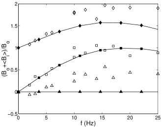
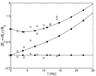
Figure 14: Comparison with the VKS experiment in the case of 2 counter-rotating TM60 propellers. Response to an axial (a) and a uniform transverse (b) magnetic field. Diamonds, squares and disks respectively refer to $B_{X}$, $B_{Y}$ and $B_{Z}$. The dark symbols and solid lines correspond to the predicted behavior based on the velocity field used in the experiment. The white symbols correspond to the measured data.

Figure 14a shows the values of the magnetic field components measured at the point P of figure 1, with an axial external field applied. On the same plot are shown the numerical results obtained for an applied field that is axial and uniform outside the cylinder and with no conducting layer. We can see that the measured values of the Y-component agree fairly well with the simulation results. The agreement is correct but not as good for the X-component of the magnetic field. Lastly, we can see that the Z-component of the measured magnetic field is significantly different from zero, its expected value. This seems to imply that the symmetry considered in paragraph 4.3.2, which forces the Z-component to zero, is somehow broken in the experiment.

The results obtained for a transverse external field are presented in Figure 14b. The transverse external field is this time uniform outside the cylinder, with no conducting layer. We can see a strong discrepancy between the measured and the simulated values of the X-component. Indeed, the measured values seem to be a factor of two larger than the computed results. On the contrary, the agreement is good for the Y-component. Finally, we can see that the measured Z-component remains in this case close to zero: either the symmetry is no longer broken in these experimental runs, or the configuration is less sensitive to dissymetry. Numerical runs have also been performed with a $W=0.2$ (see paragraph 4.1.2) conducting layer, showing only slight differences.

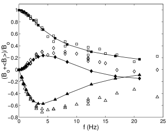
Figure 15: Comparison with the VKS experiment in the case of one rotating TM60 disk. Diamonds, squares and disks respectively refer to $B_{X}$, $B_{Y}$ and $B_{Z}$. The dark symbols and solid lines correspond to the predicted response to a uniform transverse magnetic field based on the velocity field used in the experiment. The white symbols correspond to the measured data.

Finally, figure 15 shows the results obtained in the case where only one TM60 turbine is rotating inside the vessel, the second being at rest, with a transverse field applied. The agreement is this time far better than in both the above configurations, at least for small values of the rotation rate. The Y-component of the magnetic field decreases to zero. This corresponds to an expulsion of the applied transverse magnetic field Wei66 ; Mof78 ; Odi00 . The X- and Y-components of the induced field also exhibit a quadratic dependency on the rotation frequency. Finally, we have checked numerically that the velocity field obtained for one rotating disk does not give rise to dynamo action for $R_{\rm m}<200$.

To sum up, we can see that the agreement between simulation and measurements can be satisfactory in the case where only one disk rotates, or less satisfactory in the case where both disks rotate. The good agreement in the case of one disk seems to imply that the numerical code and the measurement process are relevant. In the case where two disks rotate, however, we can see that the measurement point lies precisely at the position where the turbulence intensity is highest, and the average flow magnitude is weakest. It may be possible that the time-averaged velocity field is not sufficient to properly reproduce the experimental induction effects at this position.

5.4.2 Decay rates

It would be interesting to check the decay times presented in figure 11 against the experimental value. For the maximum value of the magnetic Reynolds number achievable in the VKS apparatus, the magnetic field energy decays in $\simeq 0.12\mu_{0}\sigma R_{c}^{2}\simeq 0.05$ s for TM60 propeller with no conducting layer. Propeller TM28 exhibits the same decay time (within 2%) at $R_{\rm m}=50$. This means that, in an experiment without conducting layer, it is very difficult to determine by pulse decay measurements alone if the turbines are of the TM28 (i.e. capable of dynamo action) or of the TM60 (i.e. incapable of dynamo action) type.

If a very large conducting layer ($W=0.2$) surrounds the experiment, however, the magnetic field energy decays in $\simeq 0.12$ s for TM28, and $\simeq 0.23$ s for TM60. In this case, it would be possible to determine which velocity field has the smallest threshold by pulse decay measurements.

5.4.3 Turbulent effects?

In the VKS apparatus, the flow shows very large turbulent fluctuations, which in turn induce very large magnetic field fluctuations Bou02 . It is expected that under certain circumstances, such fluctuations could induce a large scale component of the magnetic field through what is termed an $\alpha$-effect Mof78 . We have shown (figure 15) that, if only one propeller rotates, our numerical results are quite close to the experimental data, though the numerical simulations have been performed with the time-averaged component of the flow only. This good agreement could imply that, in that case, the leading contribution to the induction effects comes from the time-averaged component of the flow. Conversely, a discrepancy is observed in the case of two counter-rotating disks, where the time-averaged component of the flow is weaker, and where large vortices sweep the measurement location. This could possibly be ascribed to turbulence effects, either $\alpha$-effect or reduction of the electric conductivity Mof78 ; Rei01 .

6 Conclusion

The existence of dynamo effect has been recently confirmed in constrained flows in the Riga and Karlsruhe experiments. The case of experimental dynamos without internal walls remains today an open question. The numerical study of von Kármán type flows shows the possibility to have self-generation of magnetic fields for magnetic Reynolds numbers accessible to a homogeneous sodium experiment. These flows appear to be very sensitive to the precise driving configuration and to boundary conditions. The comparison of the predictions concerning the induction effects with the data of the VKS experiment exhibits paradoxical results: the agreement is excellent in the case of one disk and intermediate $R_{\rm m}$ while the results differ in the case of two counter-rotating disks. This effect could be due to the existence of the turbulent shear layer in the mid-plane, which is not accounted for in the mean velocity fields.

Tables

	$U_{pol}(ms^{-1})$		$U_{tor}(ms^{-1})$		$U_{pol}/U_{tor}$		$E_{f}$
	Mean	Max	Mean	Max	Mean	Max
TM28	0.51	1.26	0.72	1.77	0.71	0.71	0.64
TM60	0.47	1.20	0.58	0.94	0.82	1.27	0.52

Table 1: Characteristics of two experimental velocity fields corresponding to propeller TM28 and TM60. The definitions of mean and maximum velocity, poloidal and toroidal components are given in section 2.2. The efficiency corresponds to $E_{f}=U_{\rm max}/2\pi R_{c}f$.

Figure Captions

Figure 9: Imaginary part of the neutral mode growth rate $\sigma_{i}$ for $R_{\rm m}=160$ as a function of the symmetry parameter of the velocity field $\varepsilon$ as defined in the text. Symmetrized velocity field of TM 28 propeller which has a natural parameter $\varepsilon=1$, is defined on the even component of the velocity field.

References

- (1) Moffatt H. K., Magnetic field generation in electrically conducting fluids, Cambridge University Press (Cambridge 1978).
- (2) Moreau R., Magnetohydrodynamics, Kluwer Academic Publishers, Dortrecht, (1990).
- (3) Gailitis A., Lielausis O., Dement’ev S., Placatis E., Cifersons A., Gerbeth G., Gundrum T., Stefani F., Christen M., Hänel H., Will G., Phys. Rev. Lett. 84, 4365, (2000).
- (4) Gailitis A., Lielausis O., Dement’ev S., Placatis E., Cifersons A., Gerbeth G., Gundrum T., Stefani F., Christen M., Hänel H., Will G., Phys. Rev. Lett. 86, 3024, (2001).
- (5) Stieglitz R., Müller U., Naturwissenschaften, 87(9), 381-390, (2000).
- (6) Stieglitz R., Müller U., Phys. Fluids, 13, 561, (2001).
- (7) L. Marié, J. Burguete, A. Chiffaudel, F. Daviaud, D. Ericher, C. Gasquet, F. Pétrélis, S. Fauve, M. Bourgoin, M. Moulin, P. Odier, J.-F. Pinton, A. Guigon, J.B. Luciani, F. Namer and J. Léorat, MHD in von Kármán swirling flows, development and first run of the Sodium experiment. in Dynamo and Dynamics, A Mathematical Challenge, Cargèse (France) August 21-26, 2000. Eds. P. Chossat, D. Armbruster, I. Oprea, NATO ASI series, Kluwer Academic Publ. (2001).
- (8) M. Bourgoin, L. Marié, F. Pétrélis, J. Burguete, A. Chiffaudel, F. Daviaud, S. Fauve, P. Odier, J.-F. Pinton. MHD measurements in the von Kármán sodium experiment. accepted in Phys. Fluids (2002).
- (9) Dudley N.L., James R.W., Proc. Roy. Soc. Lond., A425, 407,(1989).
- (10) Ponomarenko Yu. B., J. Appl. Mech. Tech. Phys. 14, 755 (1972).
- (11) Roberts G. O., Phil. Trans. Roy. Soc. London A 271, 411 (1972).
- (12) Peffley N.L., Cawthrone A.B., Lathrop D.P., Phys. Rev. E, 61(5), 5287 - 5294, (2000).
- (13) Peffley N.L., Cawthrone A.B., Lathrop D.P., Hunting for dynamos: eight different liquid sodium flows, in Dynamo and Dynamics, A Mathematical Challenge, Cargèse (France) August 21-26, 2000. Eds. P. Chossat, D. Armbruster, I. Oprea, NATO ASI series, Kluwer Academic Publ. (2001).
- (14) Gans R.F., J. Fluid Mech. 45, 11-130 (1970)
- (15) Odier P. , Pinton J.-F., Fauve S., Phys. Rev. E, 58, 7397, (1999).
- (16) R. O’Connell, R. Kendrick, M. Nornberg, E. Spence, A. Bayliss ans C.B. Forest, On the possibibility of an homogeneous MHD dynamo in the laboratory. in Dynamo and Dynamics, A Mathematical Challenge, Cargèse (France) August 21-26, 2000. Eds. P. Chossat, D. Armbruster, I. Oprea, NATO ASI series, Kluwer Academic Publ. (2001).
- (17) P. Frick, S. Denisov, S. Khripchenko, V. Noskov, D. Sokoloff and R. Stepanov, A nonstationary dynamo experiment in a braked torus. in Dynamo and Dynamics, A Mathematical Challenge, Cargèse (France) August 21-26, 2000. Eds. P. Chossat, D. Armbruster, I. Oprea, NATO ASI series, Kluwer Academic Publ. (2001).
- (18) Picha, K. G. and Eckert, Proc. 3rd US Natl. Cong. Appl. Mech., 791-798 (1958).
- (19) Welsh, W. E. and Harnett, J. P., Proc. 3rd US Nat. Cong. Appl. Mech. (1958).
- (20) Zandbergen P. J., Dijkstra D., Ann. Rev. Fluid Mech. 19, 465 (1987).
- (21) Fauve S., Laroche C., Castaing B., J. Phys. II 3, 271 (1993).
- (22) Pinton J.-F., Labbé R., J. Phys. II (France) 4, 1461-1468 (1994).
- (23) Mordant N., Pinton J.-F., Chillà F., J. Phys. II 7, 1 (1997).
- (24) Nore C., Brachet M.-E., Politano H., Pouquet A., Phys. Plasmas 4, 1 (1997).
- (25) F. Pétrélis , M. Bourgoin, L. Marié, J. Burguete, A. Chiffaudel, F. Daviaud, S. Fauve, P. Odier, J.-F. Pinton, submitted to Phys. Rev. Let. (2002)
- (26) Alemany A., Moreau R., Sulem L., Frisch U., J. Mécanique 18, 278-313 (1979).
- (27) S. Fauve, C. Laroche, A. Libchaber, J. Phys. Lettres 42, 455 (1981) and 45, 101 (1984).
- (28) Moreau R., Sommeria, J. Fluid Mech. , (1982).
- (29) Larmor J., Rep. Brit. Assoc. Adv. Sci, 159-160 (1919).
- (30) Léorat J., Proc. Pamir Conference, Aussois(France), (1998).
- (31) D. Sweet, E. Ott, T. Antonsen and D.Lathrop, Phys. Plasmas 8, 1944-1952 (2001).
- (32) Dernoncourt, B., Pinton, J. F. and Fauve, S., Physica D, 117, 181-190 (1998).
- (33) Golitsyn, G. S., Sov. Phys. Dokl. 5, 536-539 (1960).
- (34) Moffatt H. K., J. Fluid Mech. 11, 625 (1961).
- (35) Martin A. , Odier P., Pinton J.-F., Fauve S., Eur. J. Phys. B18, 337-341 (2000).
- (36) Frisch U., Pouquet A., Léorat J., Mazure A., J. Fluid Mech. 68, 769 (1975).
- (37) Stefani F., Gerbeth G., Gailitis A., Numerical simulations for the Riga dynamo, in Laboratory Experiments on Dynamo Action, Riga (Latvia), 14-16 June 1998, Eds. O. Lielausis, A. Gailitis, G. Gerbeth, F. Stefani.
- (38) Frisch U., Turbulence, Cambridge University Press (Cambridge 1995).
- (39) Kaiser R., A. Tilgner, Phys. Rev. E 60, 2949 (1999).
- (40) Weiss N.O., Proc. Roy. Soc. A291, 60 (1966).
- (41) Odier, P., Pinton J.-F., Fauve S., Eur. Phys.J. B 16, 373 (2000).
- (42) A. Reighard, M. Brown, Phys. Rev. Let.86, 2794 (2002)