Writhing Geometry of Open DNA

Abstract

Motivated by recent experiments on DNA torsion-force-extension characteristics we consider the writhing geometry of open stiff molecules. We exhibit a cyclic motion which allows arbitrarily large twisting of the end of a molecule via an activated process. This process is suppressed for forces larger than femto-Newtons which allows us to show that experiments are sensitive to a generalization of the Călugăreanu-White formula for the writhe. Using numerical methods we compare this formulation of the writhe with recent analytic calculations.

I Introduction

Recent experiments in which DNA molecules are manipulated Strick et al. (1998); Smith et al. (1992); Cluzel et al. (1996) with the help of magnetic beads have led to a renewed interest in the statistical mechanical properties of the torsionally stiff wormlike chain Marko and Siggia (1995); Marko (1997); Moroz and Nelson (1998); Vologodskii and Marko (1997); Mézard and Bouchiat (1998). In the experiments a bead is attached to the end of a long DNA molecule; the other end remains stuck to a surface. The bead is held in a magnetic trap which allows the simultaneous application of a force, $F$ and couple, $\Gamma$; one measures the mean distance of the bead from the surface as a function of $F$ and $\Gamma$. In an ingenious theoretical paper it was shown Mézard and Bouchiat (1998) that the statistical mechanics of this problem are related to the problem of a quantum particle in a magnetic field. However, a crucial assumption was made in the formulation of the writhing geometry of the polymer.

The concept of writhe was originally defined in the context of studies on closed ribbons where it forms one part of a topological invariant, the linking number Călugăreanu (1959); White (1969). In this paper we show how the writhe can be usefully generalized to study the geometry (and the mechanical response functions) of open DNA molecules. This generalization introduces end corrections to the Călugăreanu-White formula for the writhe. We then perform simulations for the writhe distribution of an open chain which we compare with the analytic theories. We show that experiments involving manipulation of DNA with beads in unconfined geometries have unbounded fluctuations in the measured torsional angle. Under an exterior torque a bead can rotate an arbitrarily large angle. When the DNA is under tension this rotation is an activated process with jumps of $4\pi$ in the mean angle.

Contrary to the calculation performed by Bouchiat and Mézard Mézard and Bouchiat (1998) we find that this unbounded response is not removed by the introduction of an intermediate cut off. However applications of tensions larger than femto-Newtons suffice to render the problem finite in practice Rossetto and Maggs (2002). We find that their regularized expressions strongly overestimate the magnitude of writhe fluctuations for tensions larger than femto-Newtons.

In order to interpret experiments in which the molecule is under strong tension Moroz and Nelson used a Monge representation to perform a calculation of writhe fluctuations Moroz and Nelson (1998). We numerically investigate the validity of their results. We show that a strong correction to scaling can be expected due to the formation of rare loops, which give however exceptionally large contributions to the writhe. We find that the window of forces in which simple analytic theories, based on the Monge representation, are valid is rather small.

In single molecule experiments, self-avoidance confines the polymer to a single invariant knot. Analytic theories are unable to estimate the error in writhe due to summing over both knotted and unknotted configurations. We investigate this question numerically.

II Writhe and Linking Number

II.1 Closed curves

The linking number ${\mathcal{L}}k$ of a closed ribbon is an integer topological invariant Călugăreanu (1959); White (1969). It can be decomposed into two parts the twist, ${\mathcal{T}}w$ and the writhe, ${\mathcal{W}}r$:

$${\mathcal{L}}k={\mathcal{W}}r+{\mathcal{T}}w.$$ (1)

This decomposition is useful because the writhe is a function of the centerline ${\bf r}(s)$ of the ribbon.

$${\mathcal{W}}r={1\over 4\pi}\int ds\int ds^{\prime}{{\bf r}(s)-{\bf r}(s^{\prime})\over{|{\bf r}(s)-{\bf r}(s^{\prime})|^{3}}}\cdot{d{\bf r}(s)\over ds}\times{d{\bf r}(s^{\prime})\over ds^{\prime}}.$$ (2)

The linking number is invariant under deformations of the shape which do not introduce self intersections. If during a deformation the centerline ${\bf r}(s)$ crosses itself there is a discontinuity of $2$ in ${\mathcal{L}}k$ and thus, as ${\mathcal{T}}w$ is continuous, a discontinuity of 2 in ${\mathcal{W}}r$. Fuller Fuller (1971, 1978) showed the integral of equation (2) could be simplified and introduced the expression

$${\mathcal{W}}r^{F}={1\over 2\pi}\int{\hat{\bf e}_{z}\cdot({\bf t}\times\dot{\bf t})\over 1+{\bf t}\cdot\hat{\bf e}_{z}}\ ds$$ (3)

where $\hat{\bf e}_{z}$ is the direction at both extremities of the open chain. In this simplification information is lost so that ${\mathcal{W}}r$ and ${\mathcal{W}}r^{F}$ are related by the equation

$${\mathcal{W}}r-{\mathcal{W}}r^{F}=0\quad{\rm mod}\,2$$ (4)

For notational convenience let us introduced the angles, ${\chi_{C}}=-2\pi\,{\mathcal{W}}r$ and ${\chi_{F}}=-2\pi\,{\mathcal{W}}r^{F}$. A much more direct approach to Fuller’s result is possible Maggs (2001) by noting that the writhe of a stiff polymer is closely related to the geometric anholonomies discovered by Berry Berry (1987) in wave phenomena.

Equation (2) has a simple geometric interpretationArnold and Keshin (1991). The projected path of a chain on a plane with normal ${\bf u}$ can intersect itself. Each crossing is assigned a number, $\pm 1$, according to the handedness of the intersection. The sum of these numbers $n({\bf u})$ is the writhe number for direction ${\bf u}$ and the expression, eq. (2), is equal to the average of $n({\bf u})$ over all directions.

II.2 Bead rotation is given by an extended definition of writhe

The above definition of the writhe, with its emphasis on it being part of a topological invariant hides, to some degree, the interpretation of ${\chi_{C}}$ as an angle of rotation in many experimental situations. We shall now show that an extended definition of the writhe, based on equation (2) is the writhe contribution to the bead rotation that is measured in DNA twisting experiments. Rather similar arguments have also been given in Vologodskii and Marko (1997) for a polymer between two planes, we give hear an extended derivation to point out the exact limits of the result.

Consider the planar ribbon in figure 1. The linking number, ${\mathcal{L}}k$, is zero thus

$${\mathcal{W}}r+{\mathcal{T}}w=0.$$ (5)

We shall use this closed ribbon as a reference configuration to calculate the writhe of an open filament for which the initial and final tangents are parallel i.e. for ${\bf t}(0)={\bf t}(L)$, where $L$ is the polymer length. We do this using the geometry of figure 2. The polymer ${\mathcal{P}}$ which is also a ribbon is embedded in a construction consisting of two long straight sections ${\mathcal{S}}_{1}$, ${\mathcal{S}}_{2}$ and a closing loop ${\mathcal{C}}$. We shall apply eq. (2) to the constructions of figures 1 and 2 then take the length of the straight sections to infinity.

Figure 1: A flat ribbon with zero linking number.

There are beads attached to each end of the polymer, joining on to the straight sections. These two beads are our experimental reference. We shall hold the lower bead ${\mathcal{B}}_{1}$ stationary and let the upper bead ${\mathcal{B}}_{2}$ rotate due to the writhe of the polymer. The final part of our construction is the “twist absorber” ${\mathcal{T}}$. This is imagined as being a joint, or section of the straight ribbon which twists freely to absorb the writhe generated by the polymer. Let the twist of the polymer be zero so that all twist appears in ${\mathcal{T}}$.

Start from the reference state of figure 1 and deform continuously to an arbitrary state figure 2 without generating a self intersection of the construct. The writhe can be calculated with the classic double-integral. Clearly since ${\mathcal{W}}r+{\mathcal{T}}w=0$ the writhe which is generated goes into twisting the region ${\mathcal{T}}$ of the chain. The total twisting angle is just $-2\pi{\mathcal{W}}r={\chi_{C}}$. Now let the straight sections go to infinity. In this limit the contribution to the integral of the section ${\mathcal{C}}$ vanishes. Thus the experimental rotation angle is given by the ${\chi_{C}}$ for the extended construct with the two straight line sections extending to infinity .

Consider generating an ensemble of chains with some arbitrary algorithm. The distribution of the configurations of the chains is independent of the dynamic process creating them if they are subject to Boltzmann statistics. If we now choose unknotted configurations and demand that they be created via a process which preserves the linking number we conclude that we can uniquely determine the rotation angle from the writhe of the extended construct. A crucial part of this argument is the restriction of the construct of figure 2 to the sector ${\mathcal{L}}k=0$. We discuss the importance of this restriction in the next section.

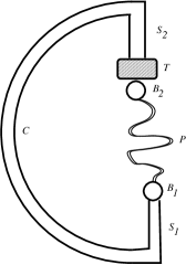
Figure 2: Deform the ribbon of figure 1 as in the diagram: The initial and final tangents of the polymer section ${\mathcal{P}}$ are parallel. Long arms ${\mathcal{S}}_{1}$ and ${\mathcal{S}}_{2}$ attach the polymer to a closing loop $C$. The experimentally important reference beads ${\mathcal{B}}_{1}$ and ${\mathcal{B}}_{2}$ are attached to the two ends of the polymer. The twist is absorbed exclusively in the section ${\mathcal{T}}$. Note the beads are not in general aligned vertically.

II.3 Choice of linking sector

In the deformation from figure 1 to figure 2 we wish to conserve the linking number ${\mathcal{L}}k$. To do so we must firstly forbid self crossing of the polymer configuration. In any experiment with DNA in the absence of topology changing enzymes this restriction in reasonable. However this condition is insufficient to conserve the topology of the entire construction. We must also forbid the crossing of the real polymer with the imaginary line from the end of the chain to infinity. In a recent numerical paper Vologodskii and Marko (1997) this was achieved by grafting the ends of the polymer to an external surface rather than beads. Experimentally we would stop this crossing by introducing a steric hindrance: A fine fiber in the neighborhood of the manipulating bead would work perfectly. We show below, however, that even this level of steric hindrance is not needed in the experiments as they are presently performed.

If the chain is allowed to bend back in such a way that is passes through the line to infinity there is a discontinuity of $\Delta\,{\mathcal{L}}k=\pm 2$. This allows one to construct a cycle of motions in which the shape of the filament undergoes a cycle coming exactly back to its original shape while the bead undergoes a rotation of $4\pi$ about the vertical axis, figure 3. This result is the origin of a common amphitheater demonstration of the importance of spinor representations of the rotation group: If one holds a plate horizontally in the palm of one’s hand one can spin it about a vertical axis by performing a suitable contortion of the arm. Against all intuition the plate can be turned an arbitrarily large angle. Photographs of Feynman performing this demonstration are to be found in Feynman (1987). Each cycle of the arm again gives rise to a rotation of $4\pi$ of the plate.

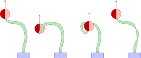
Figure 3: Demonstration of a cyclic motion of DNA leading to introduction of a twist of $4\pi$. In the first and fourth figure the shape of the molecule is identical. Between the second and third figure the vertical extension of the bead passes through the molecule leading to a discontinuity in the linking number. The tricky three dimensional geometry is most easily understood by repeating this sequence with the help of a belt or ribbon.

This unbounded torsional fluctuation is an activated process: When the DNA is under tension the bead moves against the magnetic force a distance comparable to its diameter in order to force a loop over the point of attachment. For micron sized beads this introduces a characteristic scale of the force of $k_{B}T/\mu\mathrm{m}\sim\mathrm{fN}$. For forces of more than a few femto-Newtons the process is exponentially rare and suppressed. The natural time scale for attempts at crossing the barrier is given by the Zimm time of the bead $\tau\sim d^{3}\eta/k_{B}T$ with $d$ the bead size, which is seconds.

This force is extremely low, the widely studied crossover from random coil to semiflexible behavior in the force-length characteristics of DNA occur at a force scale of $k_{B}T/\ell_{p}$ with $\ell_{p}\approx 53nm$ the persistence length of DNA. This intrinsic force scale for DNA much higher than that which is needed to conserve linking number with a $1\mu m$ bead. We conclude that most experiments with tense DNA are performed in a regime where a high energy barrier leads to conservation of the linking number of the construct of figure 2. However, there is always a small probability of passage by this barrier so that under torsion the true steady state of a DNA molecule is a state of cyclic motion in which the bead rotates by a series of activated jumps.

Because of these considerations we assume that all topological invariants are conserved during experiments, including linking number and the knot configuration of the extended construct of figure 2.

II.4 Analytic expressions for the extended writhe

From the above discussion we are lead to the calculation of the writhe of the extended construct, figure 2. The double integral, eq. (2), on the interior of the chain is identical to that commonly used for closed DNA, we denote the corresponding angle by $\chi_{int}$.

The integral from one point on the linear extension to infinity plus the second point on the polymer can be simplified as follows: The integral is evaluated by noticing that it is the spherical area, swept out by the vector

$${\bf\hat{e}}(s,s^{\prime})={{{\bf r}(s)-{\bf r}(s^{\prime})}\over{|{\bf r}(s)-{\bf r}(s^{\prime})|}}$$ (6)

as $s$ and $s^{\prime}$ vary. Consider, now, a chain, ${\bf r}(s)$. Place the origin at ${\bf r}(0)$. Let us now place $s$ in the interior of the polymer and $s^{\prime}$ on the extension of the polymer to infinity which is directed in the direction $\hat{\bf e}_{z}$. Consider, now, $s^{\prime}=0$. The curve $\hat{\bf u}(s)={\bf\hat{e}}(s,0)$ is a spherical curve. As we now let $s^{\prime}$ vary from $0$ to infinity we sweep out the area between $\hat{\bf u}$ and the point $\hat{\bf e}_{z}$. This spherical area can be written as

$$\chi_{end}=\hat{\bf e}_{z}\cdot\int\,ds\,{\hat{\bf u}\times d\hat{\bf u}/ds\over{1+\hat{\bf u}\cdot\hat{\bf e}_{z}}}.$$ (7)

then $\chi_{C}=\chi_{end}+\chi_{int}$. A similar result has been found Mézard and Bouchiat (1998) by direct integration of eq. (2). We are rather remarkably back to a problem in statistical mechanics which is very close that of the Fuller formulation, eq. (3), of the writhe fluctuations. We convert eq. (7) to spherical coordinates and find:

$$\chi_{end}=\int\,ds\,(1-\cos{\theta}){d\phi\over{ds}}$$ (8)

The singularity at $1+\hat{\bf u}\cdot\hat{\bf e}_{z}=0$ corresponds to the limit $\cos{\theta}=-1$.

II.5 Twisting

Experiments are sensitive to the sum of the writhing and twisting fluctuations in a polymer. If we now allow the excitation of the torsional modes in the polymer of figure 2 the total rotation between the two ends is the sum of the writhing angle ${\chi_{C}}$ and rotation due to internally excited twisting motions. In order to compare the twisting fluctuations to writhing fluctuations, we define $\ell_{t}=C/k_{B}T$ the torsional length, where $C$ is the torsional modulus Mézard and Bouchiat (1998). This twisting mode is unmodified by the writhing geometry, at least in the simplest models of DNA elasticity. The mean square twisting angle, $\chi_{T}$ is given by $\langle\chi_{T}^{2}\rangle={L\over\ell_{t}}$

III Artefacts in the Fuller formulation of Writhe

Recent analytic work Mézard and Bouchiat (1998); Moroz and Nelson (1998) has been based on the simplified formulation of eq. (3). It is much easier to treat analytically than the full double integral in equation (2) due to a direct mapping onto quantum mechanics: The bending energy of a stiff beam in the slender body approximation of elasticity is given by

$$E={A\over 2}\int\left({d{\bf t}(s)\over ds}\right)^{2}\ ds\ ,$$ (9)

where $A$ is the bending modulus linked to the persistence length by $\ell_{p}=A/k_{B}T$

To calculate the partition function one must now sum over all paths

$${\mathcal{Z}}=\sum_{paths}e^{-E/k_{B}T}$$ (10)

The sum for the partition function is clearly closely related to path integrals studied in quantum mechanics. Formally the energy in eq. (9) looks like the kinetic energy of a free particle moving on a sphere. From the sum of paths in equation (10) one derives a Fokker-Planck equation which is entirely analogous to the Schroedinger equation for a particle on a sphere:

$${\partial P({\bf t},s)\over\partial s}={1\over 2\ell_{p}}\nabla^{2}P({\bf t},s)\ ,$$ (11)

where $\nabla^{2}$ is the Laplacian operator on the sphere. Here $P({\bf t},s)$ is the probability of finding the chain oriented in the direction ${\bf t}$ at the point $s$. As a function of $s$ the vector ${\bf t}$ “diffuses” with diffusion coefficient which varies as $1/\ell_{p}$.

Let us now consider the writhe calculated with Fuller’s formula for such “diffusing” paths. There is a singularity in equation (3) near ${\bf t}=-\hat{\bf e}_{z}$. In the neighborhood of this direction the integral measures twice the winding of the random walk about the point $-\hat{\bf e}_{z}$. The winding of a random walk has singular properties in the two dimensional plane and on a sphere Antoine et al. (1991). In particular there is logarithmic divergence in the winding properties in the continuum limit. It is this winding number divergence that was picked up in the analytic calculation of Mézard and Bouchiat (1998) and necessitated an intermediate scale cut off in the calculation.

One of the principle conclusions of this paper is that these winding number singularities are not present in the distribution of the writhe determined experimentally: As shown above in the case of constrained linking number it is the Călugăreanu-White expression for the writhe which gives the exact twisting angle. The Fuller expression differs by an arbitrary factor of $4n\pi$ due to the winding number singularities not present in the original formulation. We shall demonstrate numerically that it is the passage from (2) to (3) which introduces these singularities. Use of (3) will be shown to lead to a substantial error in the calculation of ${\chi_{C}}$ with an overestimate by a factor of $2.5$ for a discretization corresponding to DNA.

IV Numerical Methods

Given the difficulty of treating the full Călugăreanu-White expression for the writhe analytically we decided to proceed by numerical exploration of the distributions of writhe implied by the Călugăreanu-White and Fuller formalisms. In particular we look for the Cauchy tail predicted analytically Mézard and Bouchiat (1998) in the writhe distribution function. The existence of such a tail implies the absence of a reasonable continuum limit of the wormlike chain and continuous evolution of the response functions as a function of a microscopic cut off. We shall conclude that the Călugăreanu-White formulation remains finite even in the continuum limit.

In our numerical investigations we shall be particularly interested in the fluctuations in the writhe of the open chain, as a function of the tension. Due to the algorithm used in generating the chains we are unable to generate chains in an ensemble with an imposed torsional couple. Our results are thus always for $\Gamma=0$. The torsional fluctuation are, as usual, related to the linear response of the chain via the fluctuation-dissipation theorem.

IV.1 Numerical Calculation of Writhe

A number of methods are available for the calculation of the writhe of a discretized polymer Klenin and Langowski (2000). We calculate the discretized versions of the integrals of eq. (2) and equation (3) by recognizing that they are both areas on a unit sphere. In the Fuller formulation it is the area enclosed by the curve ${\bf t}(s)$. For the discretize chain the tangent curve becomes a series of link directions, ${\bf t}_{i}$, corresponding to points on a sphere. One connects these points by geodesics and then sum over the area of the triangles formed by two successive tangent vectors and $\hat{\bf e}_{z}$.

$${\chi_{F}}=\sum_{n}{\cal A}(\hat{\bf e}_{z},{\bf t}_{n},{\bf t}_{n+1})$$ (12)

where $\cal A$ is the area of the spherical triangle defined by the three vectors.

We have already noted that the full expression, eq. (2) corresponds to the area swept out by $\hat{\bf e}(s,s^{\prime})$. For two links forming a discrete chain this defines a spherical rectangle. We calculate its area by decomposing it into two spherical triangles.

In both calculations we calculate the area of a spherical triangle by using l’Huilier’s expression

$${\cal A}=4\arctan( ( \tan((a+b+c)/4)\times$$

$$\tan((c-a+b)/4)\times$$

$$\tan((c+a-b)/4)\times$$

$$\tan((a+b-c)/4))^{1/2})$$

where, $a$, $b$ and $c$ are the lengths of the sides of a spherical triangle. For our purposes the triangle has to be oriented, the area can be either positive or negative.

A useful cross check in the programming is that for any polymer the modulo relation of eq. (4) must be satisfied despite very different intermediate results in the calculation. Numerically we found that the equality held to within $10^{-10}$, when working in double precision when the extended Călugăreanu-White definition of writhe was compared with the Fuller formulation.

Since the double integral of equation (2) is reduced to a double summation this step takes $O(N^{2})$ operations for a chain of $N$ links. For the long chains studied in our simulations it is by far the slowest step in the calculation.

IV.2 Link Sector Choice

The generation of long unknotted chains is numerically difficult; In our simulations we used an ensemble of chains with only the constraint ${\mathcal{L}}k=0$ which, as shown above, is the minimum constraint needed for unbounded torsional response. Our result can then be directly compared with existing analytic theories which do not impose any topological constraints.

The ensemble of ${\mathcal{L}}k=0$ chains may contain knots. While this ensemble may appear physically “unreasonable” one must not forget that knots are rare in the chains that we shall study. It has been noted Grosberg (2000) that for a flexible chain unknotted configurations dominate the statistics of chains even several hundred Kuhn lengths long. For the chain lengths that we work with in this paper the contamination coming from such knotted configurations should be weak. At the end of the paper we present a partial investigation of the influence of knots. We find that they do not modify our conclusions as to the nature of the continuum limit for writhing chains. The errors due to the use of a knotted ensemble are much smaller than the differences between the Fuller and Călugăreanu-White formulation of the writhe.

IV.3 Chain generation

In order to use the expressions for the writhe given above we are interested in chains in which the initial and final tangents are parallel (though the writhe for non parallel configurations does have a simple generalization Maggs (2001)) but for which there is no constraint on the final position of the chain. Rather than using a conventional Monte-Carlo algorithm to generate chains we used a simple “growth algorithm”.

IV.3.1 Zero force

We wish to grow chains of length $L$, persistence length $\ell_{p}$ using a series of links of length $b$. In the absence of tension we generate chains by starting from a single link in the $\hat{\bf e}_{z}$ direction at the origin. We then successively add links to the chain with small random angle increment $\alpha_{0}\sim\sqrt{b/\ell_{p}}$ to produce a single realization of an equilibrated semiflexible chain. It is almost certain that this chain does not satisfy the boundary conditions on the tangent thus we continue growing until the final tangent is parallel to the initial tangent to within an angle small compared with $\alpha_{0}$. We keep the polymer in our ensemble if the length of the polymer is less than $1.05\times L$, otherwise the whole configuration is rejected and the process restarted from the first link. The configurations are then used to calculate the writhing distributions. The curves that we generate are somewhat “imperfect” since they are due to a mixture of lengths. This admixture of chain lengths plays no role, however, in our analysis of the asymptotic distribution of writhe. There is no self avoidance in this code; it can be shown from a Flory argument that self avoidance is a weak effect in semiflexible chains of moderate length.

IV.3.2 Finite force

In the presence of an external force the algorithm is slightly more complicated. We proceed by noting that the partition function of a chain under tension can be expressed in a very similar manner to the partition function of a flexible polymer in an external potential Doi and Edwards (1992). We proceed by simulating the equation

$${\partial Z\over\partial s}={1\over 2\ell_{p}}\nabla^{2}Z+f\cos(\theta)\,Z\ ,$$ (14)

where $\theta$ is the angle between the direction of the force and the local tangent to the polymer, and $f=F/k_{B}T$. $Z(s,\theta)$ corresponds the number of configurations in which the chain points in the direction $\theta$ after a distance $s$.

As proposed in Velikson et al. (1992) we introduce a pool of several chains which we grow simultaneously. As each link is added there is angular diffusion as described above and a second process of birth or death of chains in the pool in order to account for the force. If $f\cos(\theta)$ is positive then it is considered to be a growth rate for reproduction of chains in the pool. If $f\cos(\theta)$ is negative the chain is stochastically destroyed with the appropriate probability. We also manage the total pool size as in Velikson et al. (1992). At the end of a pool growth, we destroy the chains that do not satisfy the condition for the tangent vector to be parallel to within $\alpha_{0}$ at both extremities.

There are several sources of error possible with the algorithm. The most difficult to evaluate is the effect of the finite pool size. The result of a single run is an ensemble of several configurations together with a total weight coming from the management of the pool size. For sufficiently large pool sizes this weight is the same for each realization of the growth process. For small pool sizes, however, this weight undergoes important fluctuations. To calculate a correlation function from an ensemble of pools we chose to select a single chain from each pool and performed a simple average over at least $10,000$ pools. Since we had no, a priory method of estimating errors from this procedure we experimented with the pool size for several different values of the force. We found that even when varying the pools size from as low as $20$ chains to $2000$ chains the estimates of the mean square writhe were stable within a few per cent. In our production runs we chose a value of $50$ chains per pool. An alternative procedure would weight each pool according to the true variation of the total weight of each simulation.

A systematic difference between a discretized chain and a continuous curve also occurs. Our principle aim is to understand experiments on DNAStrick et al. (1998); Smith et al. (1992) therefore we choose $\ell_{p}=53\,\mathrm{nm}$. We chose for $b$ the half pitch of a single helix, $1.8\,\mathrm{nm}$, yielding $\ell_{p}\simeq 30b$. This is also comparable to the diameter of the molecule. In order to study the convergence of the writhe to the continuum limit we shall also perform some simulations with $\ell_{p}/b\ \gg 30$ (see section VI.3).

V Asymptotics of Writhe in open flexible chains

Before presenting our numerical results on semiflexible chains we wish to explore the scaling behavior of the writhe of a polymer described as a freely jointed chain with $N$ links. This allows us to understand the length scales and the structures which are important in determining the writhe of a long molecule. Many of these results are already known for closed chains however we wish to demonstrate that the end corrections in eq. (7) are subdominant in the limit of very long chains.

V.1 Scaling arguments for flexible chains

We shall start with the interpretation of the writhe as a signed area swept out by the vector ${\bf\hat{e}}(s,s^{\prime})$: Consider two links $i$ and $j$ of length $a$ separated by a distance $R_{ij}$. This area scales as $A_{ij}\sim\pm(a/R_{ij})^{2}$ when $R_{ij}\gg a$. When $a\ll R_{ij}$ the area is bounded above by $2\pi$. Clearly when one averages over random walks the integral in equation (2) gives zero. The mean squared writhe can be estimated as

$$\langle{\chi^{2}_{C}}\rangle\sim\sum_{pairs}A_{ij}^{2}P(R_{ij})$$ (15)

where $P(R_{ij})$ is the pair distribution function for the polymer. For a three dimensional Gaussian polymer this function scales as

$$P(R_{ij})\sim 1/R_{ij}$$ (16)

for lengths smaller than the radius of gyration, $R_{G}\sim\sqrt{aL}$ of the polymer. Approximating the sum by an integral we find the internal contribution to the writhe,

$$\left\langle{\chi^{2}_{int}}\right\rangle\sim{L\over a^{4}}\int^{R_{G}}_{a}{a^{4}\over R^{4}}{a\over R}\quad R^{2}\,dR\sim{L\over a}$$ (17)

This integral converges at large distances, but is divergent at small distances. We conclude that the writhe integral is dominated by the cut off scale $a$. For a semiflexible polymer the cut–off $a$ corresponds to the persistence length $\ell_{p}$. It is thus the structure at this length scale which dominates the writhe of the molecule. The average crossing number is defined in a very similar manner to the writhe except the unsigned area $|A_{ij}|$ is summed over rather than the signed area. This has a non-zero mean and scales in the following way in a Gaussian polymer

$$\left\langle{\chi^{X}}\right\rangle\sim{L\over a^{4}}\int{a^{2}\over R^{2}}{a\over R}\quad R^{2}\,dR\sim{L\over a}\log{L\over a}.$$ (18)

leading to a logarithmic divergence. Thus in the crossing properties of an arbitrary projection of the polymer we expect all length scales are important.

Finally, eq. (7), the end correction to the writhe is a sum of random areas $A_{i}\sim\pm a/R_{i}$ where $R_{i}$ is now the distance between the end of the polymer and the single link $i$. The corresponding estimate of the mean square writhe is thus

$$\left\langle{{\chi^{2}_{end}}}\right\rangle\sim{1\over a^{3}}\int{a^{2}\over R^{2}}{a\over R}\quad R^{2}\,dR\sim\log{L\over a}.$$ (19)

giving a logarithmic contribution with the structure of the whole molecule being important.

When self avoidance is introduced in the problem we use the result that $P(R)\sim 1/R^{4/3}$de Gennes (1979) to show that the integral in equation (17) is still dominated by short length scales. The results for the end correction and average crossing number are however modified. They too become sensitive to structure at short wavelengths in the polymer. Thus from eq. (17) and eq. (19) the end corrections remain small for long chains and are subdominant, $\langle\chi^{2}_{int}\rangle\gg\langle\chi^{2}_{end}\rangle$.

Given the importance of this end correction in the interpretation of the experiments we now present a more rigorous study of the end correction and confirm its subdominant nature compared with the internal contributions to the writhe.

V.2 Magnitude of End Corrections

In order to further study the scaling behavior of the end corrections we examine the limit $L/\ell_{p}$ large. We thus study the problem of a freely jointed chain rather than the semiflexible chain and disprove arguments of Bouchiat and Mézard (2002) that the dominant singularities in the writhe of a semiflexible chain come from ends due to the formal analogies between eq. (3) and eq. (7). Numerical results (not shown here) on semiflexible chains lead to the same conclusions.

Let us now make a hypothesis that the asymptotics of $\chi_{end}$ are dominated by the largest contributions to the integrand of eq. (8) then

$$\chi_{end}\sim\int\,ds\,{d\phi\over{ds}}$$ (20)

which is the winding number of the polymer about $\hat{\bf e}_{z}$. The winding number of a semiflexible random walk, $W$, about an infinite line scales as

$$W^{2}\sim\log^{2}{(L/\ell_{p})}$$ (21)

where $L$ is the length of chain and $\ell_{p}$ the persistence length. The Cauchy singularity appearing in this problem is regularized by the stiffness of the chain, $\ell_{p}$.

To check this hypothesis (and to improve on the very rough scaling analysis given above, eq. (19)) we generated, figure 4, a large number of random walks for a freely jointed chain. We then plot $\sqrt{\langle{\chi^{2}_{end}\rangle}}$ as a function of $\log{L}$ and look for a straight line.

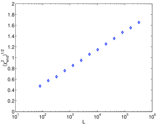
Figure 4: Variation of end correction, $\sqrt{\langle{\chi^{2}_{end}\rangle}}$ , with $L$ showing scaling identical to that of the winding of a random walk about an infinite line. Freely jointed chains with up to 320,000 links.

We conclude that the end corrections to the writhe are comparable to $\left\langle{\chi^{2}_{end}}\right\rangle=\log^{2}{(L/\ell_{p})}$. They are negligible compared with the internal contributions which vary as $\left\langle{\chi^{2}_{int}}\right\rangle\sim(L/\ell_{p})$ for $L\gg\ell_{p}$.

Despite the similarity between eq. (7) and eq. (3) we find very different scaling for $\left\langle{{\chi^{2}_{F}}}\right\rangle\sim L\log{(\ell_{p}/b)}$ and $\left\langle{\chi_{end}^{2}}\right\rangle\sim\log^{2}{(L/\ell_{p})}$. At first sight this might seem rather surprising, however in the Fuller formulation one averages over realizations of two dimensional random walks in the surface of the sphere whereas in equation (7) we average over three dimensional random walks projected onto a sphere. The statistical weights are different even if the functions are similar.

VI Writhe distribution of semiflexible polymers

VI.1 Short Molecules

For short filaments of length $L\ll\ell_{p}$ the distribution of writhe calculated with the extended Călugăreanu-White formula and the Fuller formula are indistinguishable; ambiguities due to winding about the pole are exponentially rare. The writhe distribution of a open polymer with parallel tangents at each end in the limit $L/\ell_{p}\ll 1$ is given by the Lévy Levy (1948); Maggs (2001) formula for the distribution of the area enclosed by random walk in a plane

$${P}({\chi_{C}})={\ell_{p}\over{2L}}{1\over\cosh^{2}({\chi_{C}}\,\ell_{p}/L)}\quad.$$ (22)

By generating an ensemble of $10^{6}$ short chains and binning the writhe we verified that our code was able to reproduce this result.

VI.2 Long molecules, zero tension

We have characterized the evolution of the writhe properties of a chain as a function of its length, $L$. We plot, figure 5 top, $\left\langle{{\chi^{2}_{C}}}\right\rangle$ as a function of $L$ for $\ell_{p}$ fixed. For small $L$, eq. (22), we have $\left\langle{{\chi^{2}_{C}}}\right\rangle\sim L^{2}$ and for long chains, we have $\left\langle{{\chi^{2}_{C}}}\right\rangle\sim L$, eq. (18).

As a second characteristic of the writhe distribution, figure 5 bottom, we consider $\rho_{4}=\left\langle{(x-\left\langle{x}\right\rangle)^{4}}\right\rangle/\left\langle{(x-\left\langle{x}\right\rangle)^{2}}\right\rangle^{2}$ related to the kurtosis, calculated for a probability distribution $p(x)$. If $p$ is Gaussian, then $\rho_{4}=3$. For the distribution eq. (22) $\rho_{4}=21/5$. We see numerically that $\rho_{4}=21/5$ for small $L$ and tends slowly to $3$. However, there is a large peak around $L/\ell_{p}=2$. The very strong non-monotonic behavior in figure 5 bottom is most striking; we shall now explain the origin of this feature.

Let’s call back-facing segments the sections of the chain along which ${\bf t}\cdot\hat{\bf e}_{z}<0$. We define, $n_{S}$, the number of such segments for a chain. If we compute $\rho_{4}$ with only configurations for which $n_{S}=0$ the peak disappears. We understand that the peak is due to the formation of loops in the chain which can, sometimes, completely dominate the writhing properties of a chain. Such important feature in the distribution are clearly missed in any Monge description of a chain.

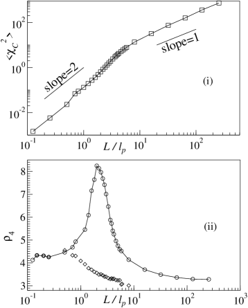
Figure 5: Top: $\left\langle{{\chi^{2}_{C}}}\right\rangle$ as a function of $L$. Bottom: $\rho_{4}$ as a function of $L/\ell_{p}$. When $L/\ell_{p}\to 0$ we find $\rho_{4}\simeq 21/5$. There is a peak around $L/\ell_{p}\simeq 2$, due to the presence of a small number of loops (typically one or two), which enlarge the probability distribution of the writhe. For larger values of $L/\ell_{p}$ $\rho_{4}\rightarrow 3$ corresponding to a Gaussian distribution. $\Diamond$ corresponds to chains with $n_{S}=0$. 100,000 chains for each point, $\ell_{p}=1000b$ for short chains and $\ell_{p}=50b$ for long chains.

From these simulations, we also estimated the coefficient of proportionality $K$ between $\left\langle{{\chi^{2}_{C}}}\right\rangle$ and $L/\ell_{p}$ for very long chains when the distribution of writhe has converged to a Gaussian:

$$\left\langle{{\chi^{2}_{C}}}\right\rangle\simeq K\frac{L}{\ell_{p}}\qquad K=2.85\pm 0.03$$ (23)

the coefficient is similar in magnitude to that found Vologodskii (2001); Klenin et al. (1989) for closed chains, even though our model for the chain is somewhat different.

VI.3 Convergence of the writhe distribution

In order to characterize the asymptotic distribution of the writhe, and study the importance of the Cauchy tail in Fuller formulation, we have performed simulations on a series of chains of length $L=8\ell_{p}$. With chains of this length knots remain rather rare whilst the energetic barrier needed for a chain oriented in the direction $\hat{\bf e}_{z}$ to wind about the direction $-\hat{\bf e}_{z}$ is only a few $k_{B}T$. We are thus sensitive to the winding singularities of the Fuller formulation. In our simulations we vary the discretization so that there are $L/\ell_{p}=$ 10, 30, 100, 300, 900, 2700 links per persistence length and we generate 200000 independent configurations for each value of $L/ell_{p}$. We plot the variance of ${\chi_{F}}$ and ${\chi_{C}}$ as a function of the discretization in figure 6. We observe a continuous evolution showing a logarithmic divergence for the Fuller formulated writhe, and a convergence to a stable value for the Călugăreanu-White form for quite moderate values of $L/\ell_{p}$. The ratio between $\left\langle{{\chi^{2}_{F}}}\right\rangle$ and $\left\langle{{\chi^{2}_{C}}}\right\rangle$ for DNA value of $\ell_{p}=30b$ is 2.4. We also see that the difference between a chain with 30 links per persistence length with the continuum limit is small (about 3%).

A divergence of the angular fluctuations implies the breakdown of linear response in the continuum limit. Since, however, $\langle{\chi^{2}_{C}}\rangle$ converges to a finite value we conclude that a microscopic cutoff is not needed to render a torsionally stiff chain finite.

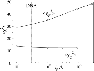
Figure 6: Variance of the writhe computed with two different formulations as a function of discretization. ${\chi_{F}}$ evolves logarithmicly, whilst ${\chi_{C}}$ converges to a constant. DNA corresponds to $\ell_{p}/b\simeq 30$, for which $\left\langle{{\chi^{2}_{F}}}\right\rangle/\left\langle{{\chi^{2}_{C}}}\right\rangle=2.4$. $L/\ell_{p}=8$, 200000 chains per point. The statistical error is smaller than symbols’ size.

VI.4 Long tense molecules

Until now we have ignored the effect of tension on the configuration of the DNA, except to remark that even very low tensions justify the use of a conserved linking number in the interpretation of the experiments. In this section we indicate how the writhe of DNA varies in the presence of external forces.

When a molecule is under high tension the molecule is largely aligned parallel to the external force. We can use a simplified, quadratic form for the Hamiltonian Moroz and Nelson (1998)

$$E={1\over 2}\int\left\{{\cal K}\left(\partial{\bf t}_{\perp}\right)^{2}+\Gamma({\bf t}_{\perp}\wedge\dot{\bf t}_{\perp}\cdot\hat{\bf e}_{z})^{2}+k_{B}Tf{\bf t}_{\perp}^{2}\right\}\quad{\rm d}s$$ (24)

where ${\bf t}_{\perp}$ describes the transverse fluctuations in the direction of the molecule. We can find the mean squared writhing angle using the usual methods of equilibrium statistical mechanics.

$$\left\langle{{\chi^{2}_{F}}}\right\rangle={\partial^{2}\log{\cal Z}\over\partial\ (\beta\Gamma)^{2}}$$ (25)

A short calculation gives

$${\left\langle{{\chi^{2}_{F}}}\right\rangle}={1\over 4}\,\sqrt{1\over f\ell_{p}}\quad\frac{L}{\ell_{p}}.$$ (26)

This expression can only be expected to be valid for forces such that $f\ell_{p}>1$.

To estimate the writhe of a molecule at low forces we return to the remark above that the internal contribution to the writhe is dominated by structure occurring at the scale $\ell_{p}$. Under low tensile forces the structure of a polymer is unchanged out to a length scale $\ell_{f}=1/f$. We conclude that under low tension, when $\ell_{f}\gg\ell_{p}$ the writhe of a molecule becomes independent of its degree of elongation and thus the tension, $f$. It is only under the highest forces when the semiflexible nature of the molecule is sampled that we see an evolution of the writhe with force.

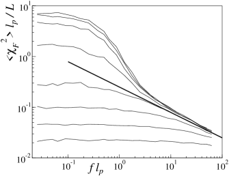
Figure 7: $\left\langle{{\chi^{2}_{F}}}\right\rangle\ell_{p}/L$ as a function of the scaled tension. At large forces the result converges to eq. (26). At low tensions the writhe is independent of the force. Simulations for $\ell_{p}=250b$. Curves for $L/\ell_{p}=$ 0.25, 0.5, 1, 2, 4, 8, 16, 32 (bottom to top). The straight line is eq. (26).

To validate our code for generating tense molecules we performed a series of simulations with a chain of persistence length $\ell_{p}=250b$, results are shown on figure 7 using the Fuller expression for the writhe. At high forces we see that the curves converge towards the law eq. (26) and that at low forces the curves saturate as expected from the above scaling argument. Somewhat surprising however is the rapid crossover which occurs for forces comparable to $f\sim 1/\ell_{p}$ when $L/\ell_{p}\gg 1$. In the neighborhood of this force there is a pronounced “shoulder” on the curve. Convergence to the long chain limit is rather slow. It is not until $L\sim 60\ell_{p}$ that we see a saturation in writhing curves. This slow convergence can be understood rather easily by noting that any chain within $\ell_{p}$ of the surface of the polymer coil is in a region of lower than average density.

We have performed a series of simulations on different levels of discretization of the polymers. We find that as the discretization becomes coarser the large shoulder dominates over the law in $1/\sqrt{f}$ for the mean square writhe. This is illustrated in figure 8 where we use 30 links per persistence length for the discrete chain. The chain of length $L=\ell_{p}$ still displays a regime in agreement with eq. (26). However with longer chains the regime in $1/\sqrt{f}$ is overwhelmed by the crossover to the low tension regime. Eq. (26) substantially underestimates the writhe fluctuations in the domain out to $f\ell_{p}=10$ corresponding to very large forces of $\sim 1\,pN$. At such forces other corrections come into play, including the chiral nature of the DNA chain.

It is interesting to note that the Fuller formulation gives results which are useful over a larger window of forces. The Fuller and Călugăreanu-White curves are very similar down to tensions $f\ell_{p}\sim 2$; analytic calculations based on the Fuller formulation can be expected to be useful for tensions larger than $0.2\,pN$. At very low forces the fluctuations are rather different. The ratio $\left\langle{{\chi^{2}_{F}}}\right\rangle/\left\langle{{\chi^{2}_{C}}}\right\rangle$ is about 2.5; use of the Fuller formulation strongly over estimates the torsional response functions.

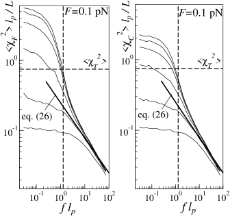
Figure 8: $\left\langle{{\chi^{2}_{F}}}\right\rangle\ell_{p}/L$ (left) and $\left\langle{{\chi^{2}_{C}}}\right\rangle\ell_{p}/L$ (right) as a function of the scaled tension. For longer chains the expected regime in $1/\sqrt{f}$ is hidden by a large shoulder from the crossover to the low force regime. Simulations for $\ell_{p}=30b$. Curves for $L/\ell_{p}=$ 1, 2, 4, 8, 16 and 32 (bottom to top). The straight bold line is equation (26). At zero force, the ratio $\left\langle{{\chi^{2}_{F}}}\right\rangle/\left\langle{{\chi^{2}_{C}}}\right\rangle$ tends to 2.5 as $L/\ell_{p}$ grows. The horizontal dashed line is the amplitude of fluctuation due to twist fluctuations when $\ell_{t}/\ell_{p}=1.5$. The vertical dashed line corresponds to $F=0.1\;\mathrm{pN}$ for DNA.

VI.5 Origin of the shoulder

To understand the origin of the shoulder which appears in figure 6 we have classified the different configurations as a function of the number of back-facing segments and computed $\left\langle{{\chi^{2}_{C}}}\right\rangle$ for subsets with $n_{S}$ fixed. The results are shown in figure 9 for $\ell_{p}/b=30$. When $f\ell_{p}\sim 1$ we see that the curves for different values of $n_{S}$ separate. $n_{S}=0$ curves do not exhibit a shoulder.

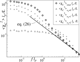
Figure 9: $\left\langle{{\chi^{2}_{C}}}\right\rangle\ell_{p}/L$ as a function of $f\ell_{p}$. Circles all chains. Triangles, averaged from no back-facing segment. We have plotted the curves for $n_{S}=1$, $\times$ and $n_{S}=2$,  ($+$). Each point computed from 300,000 configurations of length $8\ell_{p}$ with $\ell_{p}=30b$. Equation (26) solid line

The origin of the shoulder in figure 8 is essentially the same as the origin of the peak in figure 5. Under a large force, the configurations with back-facing segments are statistically rare because they have a large energy cost. Their contribution to $\left\langle{{\chi^{2}_{C}}}\right\rangle$ is, however, important.

VII Writhe and Knots

Clearly, self avoidance of the chain implies that topological invariants are constrained Bouchiat and Mézard (2002), including ${\mathcal{L}}k$. Another topological invariant that should be constrained is the knot configuration. The algorithm that we have used until now leads to an ensemble containing both knotted and unknotted chains, even if ${\mathcal{L}}k=0$. We now present a preliminary investigation on the influence of knots on the distribution of writhe. This question is related to the problem of the closure of the chain: If the polymer is allowed to pass through the line to infinity, a knot may appear, change or disappear. We thus continue with the assumption that the tension of the DNA is sufficiently high that the extended construct of figure 2 remains in the same state throughout an experiment.

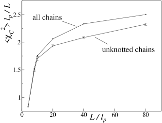
Figure 10: Fluctuations of ${\chi_{C}}$ for all chains, compared with unknotted chains, as a function of $L/\ell_{p}$. T $\left\langle{{\chi^{2}_{C}}}\right\rangle_{\text{tk}}$ is below $\left\langle{{\chi^{2}_{C}}}\right\rangle$. The knot correction lowers the fluctuations. For $L/\ell_{p}=80$ the correction computed is $-7.5\%$. ($3\sigma$) shown for $\left\langle{{\chi^{2}_{C}}}\right\rangle_{\text{tk}}$, error for $\left\langle{{\chi^{2}_{C}}}\right\rangle$ small than symbol size.

In order to select the knotted chains, we have computed the Jones polynomial $V$ Jones (1987); Kauffman (1991). The choice of the Jones polynomial is justified by the Jones conjecture, that is $V_{K}=1$ if and only if $K$ is the trivial knot. We have used the algorithm of Kauffman Kauffman (1987, 1991) to calculate $V_{K}$ and perform the classification of chains in function of their knots. Recently it has been noted that probability of knot formation is small Grosberg (2000) in short chains. Our simulations confirm this point : for chains of 8 persistence lengths the proportion of knotted chain is around $(5\pm 1)\times 10^{-4}$ when $f=0$.

To interpret a micromanipulation experiment one should perform averages over an ensemble of chains with the same given knot. In practice one hopes the experiment is performed with the trivial knot. The probability distribution of the writhe angle ${\chi_{C}}$ has to be modified, because we do not count the knotted configurations. We have computed $\left\langle{{\chi^{2}_{C}}}\right\rangle_{\text{tk}}$, where the label “tk” stands for “trivial knot” and compared it to $\left\langle{{\chi^{2}_{C}}}\right\rangle$, for different lengths with no force. Results are plotted on figure 10. The knot configurations that our algorithm generated lead to an overestimated value for $\left\langle{{\chi^{2}_{C}}}\right\rangle$. The correction is about $-7.5\%$ for the longest chains that we studied of $L=80\ell_{p}$. The correction increases the disagreement between calculations based on Fuller’s formulation of the writhe and the experimental curves. It is particularly instructive to compare figure 10 and figure 6 for the case $L/\ell_{p}=8$. Removing knots from the ensemble of chains has a negligible effect on the writhe for such short chains, however even for the most coarsely discretized chains with $\ell_{p}/b=10$ the ratio $\langle\chi_{F}^{2}\rangle/\langle\chi_{C}^{2}\rangle$ is larger than $2$. We have also studied the evolution of this correction with the force. The correction decreases rapidly with the force and is found to be zero for forces $F\ell_{p}$ larger than a few $k_{B}T$.

VIII Conclusions

In this paper we have shown that the standard experimental geometry does not torsionally confine a DNA strand so that under torque we expect an series of equivalent low energy states separated by a potential barrier. For the usual bead sizes and forces used in the experiments this barrier is very high and the extended linking number is conserved. This allows the use of an extended Călugăreanu-White formalism in the calculation of the bead rotations. We find that the Fuller and Călugăreanu-White formulae give substantially different distribution functions for the torsional fluctuations due to writhe. In contrast to Bouchiat et al. we find that the topologically confined DNA chain does not need an intermediate scale cut off to render the response functions finite. The mathematical problems as to existence of the torsional response functions occur at long wavelengths; imposing a short wavelength cut off is the wrong solution to this problem.

In experiments we expect several distinct regimes when working with beads of size $d\gg\ell_{p}$. For very low forces, $F<k_{B}T/d$ torsional fluctuations are unbounded and it is not possible to define the torsion-force-extension characteristics. In the regime $k_{B}T/d<F<k_{B}T/\ell_{p}$ torsional fluctuations are bounded but must be calculated using the full double integral representation of the writhe. The Fuller formulation, even with an additional cut off, substantially overestimates the writhe contribution to the torsional response. When $F\ell_{p}\sim k_{B}T$ a simple theory based on a Monge representation expanded to quadratic order is unable to fit the data due to strong corrections to scaling; here an expression based on the Fuller formula can be expected to give a better description of the response. Finally, for very large forces, $F\gg k_{B}T/\ell_{p}$, the Călugăreanu-White and Fuller formulae give the same result, however other effects which are neglected here become important; a full theory must treat the chiral nature of DNA and force induced denaturation.

References

- Strick et al. (1998) T. Strick, J.-F. Allemand, D. Bensimon, and V. Croquette, Biophys. J. 74, 2016 (1998).
- Smith et al. (1992) S. B. Smith, L. Finzi, and C. Bustamante, Science 258, 1122 (1992).
- Cluzel et al. (1996) P. Cluzel, A. Lebrun, C. Heller, R. Lavery, J.-L. Viovy, D. Chatenay, and F. Caron, Science 271, 792 (1996).
- Marko and Siggia (1995) J. Marko and E. D. Siggia, Phys. Rev. E 52, 2912 (1995).
- Marko (1997) J. Marko, Phys. Rev. E 55, 1758 (1997).
- Moroz and Nelson (1998) J. Moroz and P. Nelson, Macromol. 31, 6333 (1998).
- Vologodskii and Marko (1997) A. Vologodskii and J. Marko, Biophys. J. 73, 123 (1997).
- Mézard and Bouchiat (1998) M. Mézard and C. Bouchiat, Phys. Rev. Lett. 80, 1556 (1998).
- Călugăreanu (1959) G. Călugăreanu, Rev. Math. Pures Appl. 4, 5 (1959).
- White (1969) J. White, Am. J. Math. 91, 693 (1969).
- Rossetto and Maggs (2002) V. Rossetto and A. C. Maggs, Phys. Rev. Lett 88, 089801 (2002).
- Fuller (1971) F. B. Fuller, Proc. Nat. Acad. Sci. U.S.A. 68, 815 (1971).
- Fuller (1978) F. B. Fuller, Proc. Nat. Acad. Sci. U.S.A. 75, 3557 (1978).
- Maggs (2001) A. C. Maggs, J. Chem. Phys. 114, 5888 (2001).
- Berry (1987) M. Berry, Nature 326, 277 (1987).
- Arnold and Keshin (1991) V. I. Arnold and B. A. Keshin, Topological methods in hydrodynamics (Springer–Verlag, 1991).
- Feynman (1987) R. P. Feynman, Elementary particles and the laws of physics: the 1986 Dirac memorial lectures. (Cambridge University Press, 1987).
- Antoine et al. (1991) M. Antoine, A. Comtet, J. Desbois, and S. Ouvry, J. Phys. A. 24 (1991).
- Klenin and Langowski (2000) K. Klenin and J. Langowski, Biopolymers 54, 307 (2000).
- Grosberg (2000) A. Y. Grosberg, Phys. Rev. Lett. 85, 3858 (2000).
- Doi and Edwards (1992) M. Doi and S. Edwards, The Theory of Polymer Dynamics (Clarendon, Oxford, 1992).
- Velikson et al. (1992) B. Velikson, T. Garel, J.-C. Niel, H. Orland, and J. C. Smith, J. Comput. Chem. 13, 1216 (1992).
- de Gennes (1979) P.-G. de Gennes, Scaling concepts in polymer physics (Cornell University Press, New York, 1979).
- Bouchiat and Mézard (2002) C. Bouchiat and M. Mézard, Phys. Rev. Lett. 88, 089802 (2002).
- Levy (1948) P. Levy, Processus Stochastiques et Mouvement Brownien (Editions Jacques Gabay, 1948).
- Vologodskii (2001) A. V. Vologodskii, Molecular Biology 35, 240 (2001).
- Klenin et al. (1989) K. V. Klenin, A. V. Vologodskii, V. V. Anshelevich, V. Y. Klisko, A. M. Dykhne, and M. D. Frank-Kamenetskii, J. Biomol. Struct. Dyn. 6, 707 (1989).
- Jones (1987) V. F. R. Jones, Ann. of Math. 126, 335 (1987).
- Kauffman (1991) L. H. Kauffman, Knots and physics (World Scientific, 1991).
- Kauffman (1987) L. H. Kauffman, Topology 26, 395 (1987).