Abstract

We developed analytical technique for extracting the phase, visibility and amplitude information as needed for interferometric astrometry with the Space Interferometry Mission (SIM). Our model accounts for a number of physical and instrumental effects, and is valid for a general case of bandpass filter. We were able to obtain general solution for polychromatic phasors and address properties of unbiased fringe estimators in the presence of noise. For demonstration purposes we studied the case of rectangular bandpass filter with two different methods of optical path difference (OPD) modulation – stepping and ramping OPD modulations. A number of areas of further studies relevant to instrument design and simulations are outlined and discussed.

OCIS codes: 120.2440, 120.2650, 120.3180, 120.5050, 120.5060

Introduction

SIM is designed as a space-based 10-m baseline Michelson optical interferometer operating in the visible waveband (see Ref. 1 for more details). This mission will open up many areas of astrophysics, via astrometry with unprecedented accuracy. Thus, over a narrow field of view SIM is expected to achieve mission accuracy of 1 $\mu$as. In this mode SIM will search for planetary companions to nearby stars by detecting the astrometric “wobble” relative to a nearby ($\leq 1^{\circ}$) reference star. In its wide-angle mode, SIM will be capable to provide a 4 $\mu$as  precision absolute position measurements of stars, with parallaxes to comparable accuracy, at the end of a 5-year mission. The expected proper motion accuracy is around 3 $\mu$as/yr, corresponding to a transverse velocity of 10 m/s at a distance of 1 kpc.

The SIM instrument does not directly measure the angular separation between stars, but the projection of each star direction vector onto the interferometer baseline by measuring the pathlength delay of starlight as it passes through the two arms of the interferometer. The delay measurement is made by a combination of internal metrology measurements to determine the distance the starlight travels through each arm, external metrology measurements that determine the length and local orientation of the baseline, and a measurement of the central white light fringe to determine the point of equal optical pathlength (see Figure 1).

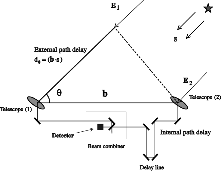
Fig. 1: Basic geometry of light propagation in the stellar interferometry.

The primary motivation for the work was the idea to use the averaged and bias-corrected complex phasors to estimate the external optical pathlength difference for the incoming polychromatic light. This approach is applicable to the science interferometer phase measurement, for which it is not necessary to remove the bias from each estimate, just as long as it is removed from the averaged estimate. This method was applied in Ref. 2 to obtain unbiased fringe visibility estimates. Under certain conditions (dc intensity values and visibilities approximately constant during integration time) this method allows to use the average values of the phasors for estimating the average phase $\bar{\phi}$ (see discussion in Refs. 3, 4). A definition for the complex visibility phasors is stemming from the form of a complex visibility function, $\tilde{V}=ve^{j\phi}$, where $v$ is the visibility and $\phi$ is its phase. Decomposing this expression onto real and imaginary parts as $\tilde{V}=X+jY$, one obtains the complex visibility phasors, $X=v\cos\phi$ and $Y=v\sin\phi$. SIM will be able to effectively determine both visibility and phase of the fringe, but for the astrometric purposes the phase must be determined to a much higher accuracy. (The most stringent SIM requirement in this regard is the average phase error over 30 s integration time corresponds to a path-length error of approximately 30 pm.) Phase determination in the presence of noise is a non-linear estimation process. Even in the monochromatic case it requires careful approach to averaging and correcting for biases in the data. Most of the algorithms for phase-shifting interferometry are designed for monochromatic light, and there is typically a match between the stroke of the modulating element and the wavelength of the light (see, for example, Refs. 5 for a discussion of various algorithms). However, because SIM uses a dispersed fringe technique, this match cannot be maintained over multiple channels. A number of modifications to the existing four-bucket algorithms were designed to address specific problems relating to Palomar Testbed Interferometer (PTI)[6] and the Keck Interferometer. Also, there is nothing inherent that requires the match between wavelength and stroke, nevertheless most analysis has been based on this assumption. It was shown in Ref. 4 that at low light levels, most of these algorithms become biased when there is a mismatch. The magnitude of this bias is quite significant with respect to the instrument requirements, thus making these algorithms unacceptable for SIM.

This paper discusses analytic model developed for the white light fringe data extraction. Our goal here is to establish functional dependency of the white light fringe parameters on the properties of incoming light as well as the instrumental input parameters. We will show that this approach is applicable for establishing the unbiased estimators for the case with low light levels. This method enables on to analytically analyze the noise propagation properties. The importance of this feature comes from the fact that integration time on stellar targets accounts for a significant portion of the mission time and can be reduced by the use of processing techniques with reduced error variance (see Refs.7-10 for more details). The analytical from of the fringe parameters may be helpful in studying different properties of the instruments, especially their contribution to the accuracy of astrometric delay measured by SIM science interferometer.[11, 12]

The problem of interference of electromagnetic radiation is well studied and extensive number of publications on this subject (specifically related to stellar interferometry) are available (see Refs. 10,13-19 and references therein). However, because of complexity of this problem in a general case of polychromatic light, most of the current research is done numerically. While numerical studies have proven to be extremely valuable in analyzing the interference patterns and are very useful in addressing various instrumental effects, the analytical methods provide the much needed critical understanding of the white light interference phenomena. It will be demonstrated below that analytic solution may be used as a tool to study the complex interferometric phenomena on a principally different qualitative level.[3]

In this paper we derive analytic model that may be used to describe photo-electron detection process. We analytically describe the physical and instrumental processes that are important in estimating the fringe parameters (i.e. intensity of incoming radiation, its visibility and the phase of the fringe). Effects that are not included in the model are due to polarization of both incoming light and the instrumental throughput, effect of the wavefront-tilt, low frequency vibrations, drifts, jitter, etc. Consideration the size of this paper, we plan to address these issues elsewhere.

The paper is organized as follows: In Section 1 we review the description of interferometric pattern in the case of monochromatic radiation. In Section 2 we develop a model for the interferometric pattern registered by a CCD detector in the polychromatic case. Our model accounts for the effects of the instrumental throughput, beam splitter and quantum efficiency of the CCD. We also discuss the spectral channels with narrow bands designed to filter the polychromatic light. In Section 3 we introduce parameterization for the polychromatic fringe pattern and define the quantities that are forming the astrometric signal on the CCD. Specifically, we derive solution for the white light fringe equation in the general case. In Section 4 we present general analytic solution for complex visibility phasors and will discuss a noise suppression approach. In Section 5 we develop technique for studying the case of a rectangular bandpass filter. We also obtain functional dependency of our solution in the two cases of OPD modulation, namely the stepping and ramping modulations. In Section 6 we present conclusions and recommendations for future studies of accurate fringe reconstruction. In order to make access of the basic results of this paper easier, we will present some important calculations in the Appendices. Thus, in Appendix A we discuss two possible definitions for the fringe phase and justify the choice we made in the paper. In Appendix B we develop approximation for the complex fringe envelope function. In Appendix C we present a general solution for the instrumental contribution affecting the fringe parameters in the case of the rectangular bandpass filter and stepping OPD modulation.

1 Monochromatic Fringe Pattern

The problem of interference of a monochromatic radiation presently is well studied (see Ref.13 and references therein). Here we would like to review information that will be necessary for discussion of the fringe phase extraction process.

We assume that a plane electromagnetic wave, $\vec{E}$, which is coming from infinity simultaneously on the two arms of an interferometer, has the following form:

$$\vec{E}=\vec{E}_{0}e^{j\,\big{(}\omega t-{\vec{k}}\cdot{\vec{x}}\big{)}},$$ (1)

with $\vec{E}_{0}$ is a constant vector. We will be using a nomenclature where a wavenumber $k$ relates to the wavelength as follows $k=\frac{2\pi}{\lambda}$. After passing through the interferometer, the two beams $\vec{E}_{1}$ and $\vec{E}_{2}$, are combined at the detector to produce interferometric pattern (see Figure 1). The corresponding fringe pattern is due to the coherent addition of the two light-beams, $\vec{E}=\vec{E}_{1}+\vec{E}_{2}$, and it may be expressed as follows:

$${\cal I}=\langle\vec{E}\cdot\vec{E}^{*}\rangle_{\sf time}={\vec{E}^{2}}_{01}+\vec{E}^{2}_{02}+2\langle\vec{E}_{1}\vec{E}_{2}\rangle,$$ (2)

where ^∗ denotes a complex conjugate quantity and $\langle..\rangle_{\sf time}$ denotes a time-averaged quantity. The first two terms on the right-hand side of this equation are constant intensities of light in the two beams, ${\cal I}_{1}={\vec{E}^{2}}_{01}$ and ${\cal I}_{2}=\vec{E}^{2}_{02}$. The third one is the interferometric pattern which, in ideal situation, depends only on the optical path difference between the two beams and the wavelength of the radiation, namely $\phi_{0}=\phi_{1}-\phi_{2}=\frac{2\pi}{\lambda}d_{0}\equiv kd_{0}$. The resulting intensity of radiation on is given

$${\cal I}(k)={\cal I}_{0}\big{(}1+V\cos kd_{0}\big{)},$$ (3)

where we denote the constant part in the intensity pattern as ${\cal I}_{0}={\cal I}_{1}+{\cal I}_{2}$. Also, the quantity $V$ is the visibility of the incoming light, which, in the case of the beams intensities mismatch ${\cal I}_{1}\not={\cal I}_{2}$, is given by[13, 16]

$$V=\frac{2\sqrt{{\cal I}_{1}{\cal I}_{2}}}{{\cal I}_{1}+{\cal I}_{2}}{\cal V}=\frac{2|\vec{E}_{01}||\vec{E}_{02}|}{\vec{E}^{2}_{01}+\vec{E}^{2}_{02}}{\cal V}.$$ (4)

The factor ${\cal V}$ ($0\leq{\cal V}\leq 1$) in this equation is the true source visibility (or the fringe contrast). In the case of monochromatic radiation from an un-resolved source, when the intensities in the two arms of the interferometer are of equal amplitudes, or $|\vec{E}_{01}|=|\vec{E}_{01}|=E_{0}$, the constant intensity becomes ${\cal I}_{1}={\cal I}_{2}=\frac{1}{2}{\cal I}_{0}$. Therefore, visibility reduces simply to one, $V=1$.

A Fringe Modulation

As seen in Figure 2 monochromatic pattern is a simple one. In practice, the studied source may be interferometrically resolved, thus leading to a reduced visibility $V\not=1$. Moreover, the visibility $V$, the constant phase difference $\phi_{0}$ and the constant intensity ${\cal I}_{0}$ are generally not known. To find them one modulates the phase difference with some known function, say $x(t)$, as below:

$${\cal I}(k,t)={\cal I}_{0}\Big{(}1+V\sin\big{(}\phi_{0}+k\,x(t)\big{)}\Big{)},$$ (5)

where effect of the beam splitter (which is true for a Michelson stellar interferometer) brings additional $\frac{\pi}{2}$ phase shift (discussed in Section 2B).[6, 8, 9]

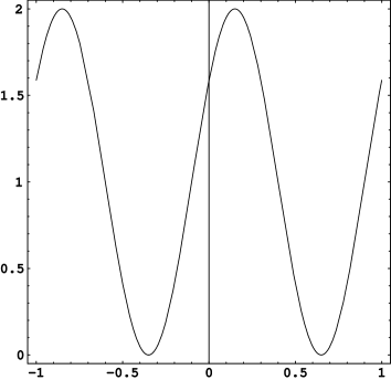
Optical pathlength difference, $x$

Fringe amplitude

Fig. 2: Monochromatic fringe. Note the visibility is set $V=1$ and the initial phase offset chosen to be $\phi_{0}=\frac{\pi}{5}$.

The primary goal here is to determine the phase $\phi_{0}$ by modulating the internal optical path difference $x(t)$. By doing so, one finds the exact value of internal delay $x_{\sf int}=x(t^{\prime})$ that would exactly compensate the initial offset or $k(d_{0}-x_{\sf int})=0.$ Then, having determined the external delay $d_{0}=x_{\sf int}$ one can determine the source position from equation $d_{0}=({\vec{b}}\cdot{\vec{s}})$, where ${\vec{b}}$ is the interferometer baseline vector and ${\vec{s}}$ is the source position on the sky. In practice, this is done in a global astrometric solutions discussed in details in Refs.11, 12 and not addressed here.

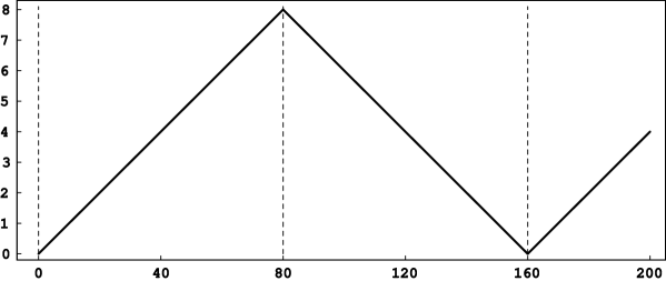
Time, [ms]

Temporal bins

Fringe amplitude

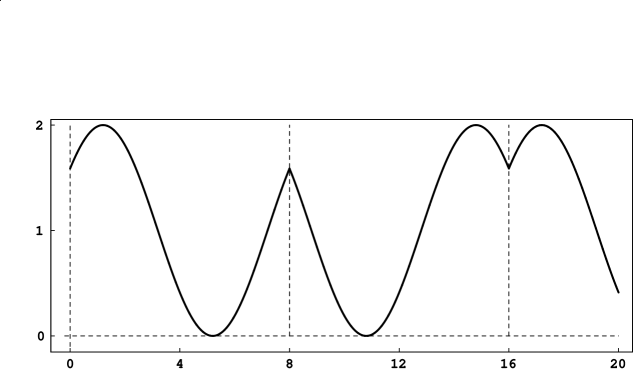
Optical pathlength difference, [bins]

Fig. 3: Upper plot shows a typical OPD modulation stroke with ramping over 8 equal temporal bins with duration of 10 ms each. Lower plot is a monochromatic fringe as a function of OPD that is modulated by ramping over a wavelength (initial phase offset is $\phi_{0}=\frac{\pi}{5}$ - same as in Figure 2).

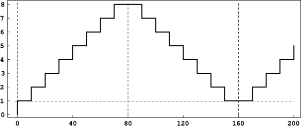
Time, [ms]

Temporal bins

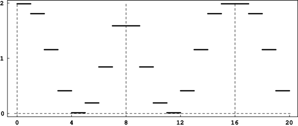
Optical pathlength difference, [bins]

Fringe amplitude

Fig. 4: Upper plot shows typical OPD modulation stroke with stepping over 8 equal temporal bins with duration of 10 ms. Lower plot is a monochromatic fringe as a function of OPD modulated in 8 equal steps over a wavelength, as shown in the upper plot. (The fringe parameters the same as in Figure 2.)

As shown in the Figures 3 and 4 there may be different ways of modulating the internal OPD in an interferometer. In particular, Figure 3 demonstrates the case when the OPD is modulated linearly. Thus, the upper plot shows a typical phase change with ramping over 8 equal temporal bins with duration of 10 ms each. The lower plot shows the same monochromatic fringe shown in Figure 2 as a function of OPD that is modulated by ramping over a wavelength. Note the difference between this case and the case shown in Figure 4, where the upper plot shows a typical phase modulation provided by the stepping OPD modulation with the stroke stepping over 8 equal temporal bins with duration of 10 ms each. The lower plot in this Figure demonstrates behavior of monochromatic fringe as a function of OPD with modulated stroke stepping in equal steps over a wavelength as shown in the upper plot.

The photon count on the detector, $N$, is proportional to the intensity, $N\propto{\cal I}$. Therefore, by collecting photons $N_{i}(k)\sim{\cal I}(k,t_{i})$, coming at the detector at a certain time intervals $t_{i}\in[t_{i}^{-},t_{i}^{+}]),~{}i\in[1,..,N]$ (or by integrating Eq. (5) over $dt$ from $t_{i-1}$ to $t_{i}$), one forms the system of equations to determine the unknown quantities ${\cal I}_{0}$, $V$ and $\phi_{0}$. These time intervals correspond to different values of OPD, $x(t)\in\Big{\{}x_{i},~{}i\in[1,..,N]\Big{\}}$, therefore, observational equation in the case of monochromatic light and ramping OPD modulation takes the following form:

$${\cal I}_{i}(k)={\cal I}_{0}\Big{(}1+V{{\rm sinc}\,[\frac{1}{2}kv\,\Delta\tau_{i}]}\sin\big{(}\phi_{0}+k\,x_{i}\big{)}\Big{)},$$ (6)

where ${\rm sinc}(\cdot)$-function is given as usual ${\rm sinc}\,z=\sin z/z$; $v$ is the constant velocity of OPD modulation stroke, $x(t)=vt$ and $\Delta\tau_{i}=t_{i}-t_{i-1}$ is the integration time for the $i$-th temporal bin.

Eq. (6) is the most studied equation when estimating the fringe parameters in the monochromatic light approximation. Solution to this equation is quite straightforward and it was extensively discussed in literature (see, for example, Ref.5, 15). Usually, Eq. (6) is represented in a matrix form as ${\cal I}_{i}=A_{i\alpha}X^{\alpha}$, where indexes $i$ and $\alpha$ running as $i\in\{1,...,N\}$ and $\alpha\in\{1,2,3\}$. Vector $X^{\alpha}$ is the to-be-determined phasors vector given as $X^{\alpha}=\big{(}{\cal I}_{0};\,{\cal I}_{0}V\cos\phi_{0};\,{\cal I}_{0}V\sin\phi_{0}\big{)}^{T}$. Matrix ${\bf A}^{T}=A_{i\alpha}=\Big{(}1;\,{{\rm sinc}\,[\frac{1}{2}kv\,\Delta\tau_{i}]}\sin kx_{i};\,{{\rm sinc}\,[\frac{1}{2}kv\,\Delta\tau_{i}]}\cos kx_{i}\Big{)}$ is the $3\times N$ matrix of 3D rotation in the phase space. A solution to this equation is given by $X^{\alpha}={A^{\dagger}}^{i\alpha}{\cal I}_{i},$ where ${{\bf A}^{\dagger}}=({\bf A}^{T}{\bf A})^{-1}{\bf A}^{T},$ with ${{\bf A}^{\dagger}}$ being the pseudo-inverse of ${\bf A}$. This set of equations may be solved uniquely only in the case when $N=3$. For all other cases, when $N>3$, the obtained system of equations is over-determined, and one obtains a least-squares solution by constructing pseudo-inverse matrix ${{\bf A}^{\dagger}}$.[3, 5, 15] We will discuss an optimally-weighted, noise optimized solution to this set of equations in more details in Section 4, while dealing with a more complicated case of the polychromatic light.

When dealing with a polychromatic light content in the wide bandwidth, one either i) forms a light with a narrow spectral width, such that effects of polychromacity (discussed further) are negligible, or ii) disperses the light beam on a large number of spectral channels, such that monochromatic approximation is valid within each channel.[16] As a result, most of the current algorithms and simulations for stellar optical interferometry are based on the properties of the monochromatic light. This is a good approximation for some of existing testbed configurations that use as many as 80 spectral channels for dispersed light. Nominally the SIM flight system will use four to eight channels for guide interferometers. Because of the large bandwidth of each channel (87.5 nm), the quasi-monochromatic assumptions are not valid, and modifications to the algorithms are necessary.[4, 19] In the following Section we will introduce a method designed to address this issue.

2 Modeling Observables for a Polychromatic Fringe

The observational conditions in the case of polychromatic light are significantly altered compare to the simplicity of the monochromatic situation discussed in Section 1. Thus, Figure 5 shows a general behavior of harmonic signals with a different frequencies. The left plot in the figure shows three sinusoidal monochromatic waves with the same initial phase offset $\phi_{0}=\pi/5$. Depending on the wavenumber, each wave, as a function of OPD, produces different fringe pattern. Note that a combination of these three waves (a simple model of a polychromatic fringe) also produces a harmonic signal, but its shape is drastically different from the initial one (shown on the right plot). For the expected SIM finite bandwidth the wavenumbers of the interfering light may be different as much as twice from each other (i.e. the SIM wavenumber bandwidth is $k\in[450,950]$ nm). Thus, in general, only at zero OPD (i.e. for the white light fringe) the interferometric pattern would have maximum intensity.

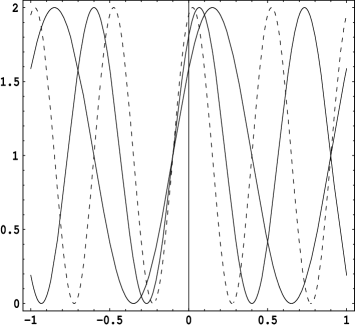
Optical pathlength difference, $x$

Fringe amplitude

Fringe amplitude

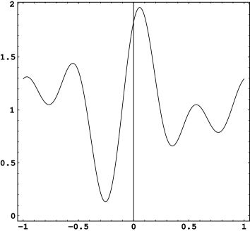
Optical pathlength difference, $x$

Fig. 5: Left plot shows three independent monochromatic waves presented as a functions of the OPD. The phase of the fringes is changing as $\phi=\phi_{0}+k_{i}x$, with external delay corresponding to a phase difference of $\phi_{0}=\frac{\pi}{5}$ and three wavenumbers chosen $k_{1}=k_{0},~{}k_{2}=1.5k_{0},~{}k_{3}=2k_{0}$ (thus the bandwidth is $\Delta k=k_{0}$), where $k_{0}$ is a reference wavenumber. The right plot represents the interference pattern of polychromatic light composed from the same three sinusoidal waves shown on the left plot. Note the drastic change in the character of the interferometric pattern.

In this Section we will derive an equation to describe the interference pattern of a polychromatic fringe as needed for the SIM CCD detector read-out.

A Modeling Observables in the Wide Bandwidth Case

As was mentioned earlier, the case of describing interferometric pattern that involves a finite bandwidth - is a more complicated one. In general all the quantities involved are complicated functions of a wavenumber. Note that, contrary to the Eq. (1), not only the phase of the electromagnetic wave depend on time and wavelength, but the same true on it’s amplitude

$$\vec{E}(k,t)=\vec{E}_{0}(k,t)e^{j\,(\omega t-kx)},$$ (7)

with $\vec{E}_{0}$ being the wave’s amplitude vector that depends both on the wavelength and time. This expression shows a wave-packet that describes individual contribution to the polychromatic light that is due to a particular monochromatic constituent of it.

A way to describe this process is to collect all constituents of polychromatic light at different wavelengths that are present in the incoming electromagnetic wave. It is convenient to express the intensity of the polychromatic radiation as a coherent addition of the individual wave-packets (1) with a different frequencies [13]. Denoting ${\vec{E}}_{01}$ and ${\vec{E}}_{02}$, to represent the light coming onto a detector from the two arms of interferometer, this procedure may functionally be expressed in the following form:

$${\cal I}(k,t) \sim \Big{\langle}\big{(}{\vec{E}}_{01}(k,t)+{\vec{E}}_{02}(k,t)\big{)}\cdot\big{(}{\vec{E}}^{*}_{01}(k,t)+{\vec{E}}^{*}_{02}(k,t)\big{)}\Big{\rangle}_{\sf time}=$$ (8)

$$= {\vec{E}}^{2}_{01}(k)+{\vec{E}}^{2}_{02}(k)+2|{\vec{E}}_{01}(k)||{\vec{E}}_{02}(k)|\gamma(k)\cos\Big{(}\Phi(k)+\Delta\varphi_{12}(k,t)\Big{)},$$

where $\Delta\phi_{12}(k,t)$ is the external phase difference between the two arms of interferometer and $\tilde{\gamma}(k)=\tilde{\cal V}(k){\tilde{T}}(k)=\gamma(k)e^{j\,\Phi(k)}$ is the complex coherency factor.

This complex coherency factor includes both - the true complex visibility of the source, $\tilde{\cal V}(k)$, and the complex instrumental transfer function denoted as ${\tilde{T}}(k)$. The complex source visibility function is given in its usual form

$$\tilde{\cal V}(k)={\cal V}(k)e^{j\,\phi_{\cal V}(k)},$$ (9)

with ${\cal V}(k)$ being the amplitude and $\phi_{\cal V}(k)$ the phase of the true source visibility. According to Van-Cittert-Zernike theorem, namely this quantity is connected to the true radiation emitted by a star. Specifically, this theorem allows to calculate mutual intensity observed on a surface some distance from the source [13]. The instrumental complex transfer function, ${\tilde{T}}(k)$, may also be presented in a similar manner

$${\tilde{T}}(k)=T(k)e^{j\,\phi_{T}(k)},$$ (10)

with $T(k)$ being the amplitude of this function and $\phi_{T}(k)$ its phase. Therefore, the complex coherency factor ${\tilde{\gamma}}(k)$, that is present in the equation (8), has the following functional dependency:

$$\tilde{\gamma}(k)=\tilde{\cal V}(k){\tilde{T}}(k)={\cal V}(k)T(k)e^{j\,[\phi_{\cal V}(k)+\phi_{T}(k)]}\equiv\gamma(k)e^{j\,\Phi(k)},$$ (11)

where combined apparent visibility and phase are given by the expressions $\gamma(k)={\cal V}(k){T}(k)$ and $\Phi(k)=\phi_{\cal V}(k)+\phi_{T}(k)$ correspondingly.

The modulated phase difference $\Delta\varphi_{12}(k,t)$ in the Eq.(8) may be expressed in terms of the internal pathlength difference:

$$\Delta\varphi_{12}(k,t)=kx(t),$$ (12)

with $x(t)=\ell_{1}(t)-\ell_{2}(t)$ being the internal pathlength difference between the two arms of interferometer (see Figure 1).

Let us define individual spectral densities of photon flux in each arm of interferometer as ${\cal I}_{1}\sim{\vec{E}}^{2}_{01}(k)$ and ${\cal I}_{2}\sim{\vec{E}}^{2}_{02}(k)$. This allows us to present the intensity of incoming radiation at a particular wavenumber $k$ as

$${\cal I}(k,t)\sim{\cal I}_{1}(k)+{\cal I}_{2}(k)+2\sqrt{{\cal I}_{1}(k){\cal I}_{2}(k)}\,\gamma(k)\cos\big{(}\Phi(k)+kx(t)\big{)}.$$ (13)

It is naturally to define the total spectral density of photon flux of light approaching the detector as ${\cal I}_{0}(k)={\cal I}_{1}(k)+{\cal I}_{2}(k)$. Note that individual spectral densities of photon flux in the two arms of interferometer, ${\cal I}_{1}$ and ${\cal I}_{2}$, may be different. To account for such a mismatch we introduce apparent visibility ${\tilde{V}}(k)$

$${\tilde{V}}(k)=\frac{2\sqrt{{\cal I}_{1}(k){\cal I}_{2}(k)}}{{\cal I}_{1}(k)+{\cal I}_{2}(k)}\gamma(k)=V(k)e^{j\,\Phi(k)}.$$ (14)

The resulted expression for the spectral density of photon flux of the incoming radiation at a particular wavenumber $k$ takes the following form:

$${\cal I}(k,t)={\cal I}_{0}(k)\Big{(}1+V(k)\cos\big{(}\Phi(k)+kx(t)\big{)}\Big{)}.$$ (15)

Furthermore, the energy density of incoming polychromatic radiation per a unit wavenumber may be obtained by integrating the photon flux at the detector Eq. (15) over the wavenumber space $dk$:

$$d{\cal I}(k,t)={\cal I}_{0}(k)\Big{(}1+V(k)\cos\big{(}\Phi(k)+kx(t)\big{)}\Big{)}dk.$$ (16)

Expression (16) defines the energy density of the interfering light per a unit wavenumber. The quantity that is proportional to it, namely the photo-electron count, will be registered by a CCD detector via a photo-electron emission process and will be discussed in Section 2C.

B Effect of a Beam Splitter

To complete the formulation of our model we need to account for yet one more element that is of crucial importance for a Michelson stellar interferometer - the beam splitter.[6, 9] It is well-known that one of the figures of merit when considering various beam splitter designs for the astrometric beam combiner, is the variation of phase as a function of wavelength between the interfering beams at zero OPD. Thus, ideally, one would like zero phase difference for all wavelengths at zero OPD since this would produce a fringe maximum simultaneously at all wavelengths (or fringe minimum for a Michelson stellar interferometer). Another desirable case is one in which the phase difference varies linearly with frequency. In this case one can still achieve a simultaneous fringe maximum at all wavelengths; however, for this case there is a constant correction that must be applied to the calculated external delay. [3]

This effect is important because it may produce a significant contribution to the OPD. We may include this effect in a most general way — the wavenumber dependent function $f(k)$ added to the desirable $\pi/2$ effect of an ideal beam splitter. Thus, the total effect of the beam splitter may be modeled as

$$\delta\Phi_{\sf bs}(k)=\frac{\pi}{2}+f(k),$$ (17)

where $f(k)$ is a slow varying function of a wavenumber. This function may be approximated up to the second order around some central frequency of bandpass (the whole 80 channels pass), $k_{c},$ as

$$f(k)=f(k_{c})+f^{\prime}(k_{c})(k-k_{c})+\frac{1}{2}f^{\prime\prime}(k_{c})(k-k_{c})^{2}+{\cal O}(\Delta k^{3}_{c}).$$ (18)

It may be shown[3] that function $f(k_{c})$ will have a direct impact on the phase accuracy estimation by shifting the phase by a constant value. In addition, the function $f^{\prime}(k_{c})$ will change the envelope function and, in general, will produce a non-linear contribution to the phase. $f^{\prime\prime}(k_{c})$ will have impact on both - linear contribution to the phase and the non-linear one; first it comes as a correction to the envelope function and then to the phase. Even though, the magnitude of the effects of $f^{\prime\prime}$ is smallest among all, the parameters $f,f^{\prime},f^{\prime\prime}$ are all of importance. The corresponding effects may be well modeled, depending on the optical properties of the beam splitter, but the final answer would come probably form calibration.

Finally, without loosing generality, the effect of beam splitter may be accounted for as an additional phase shift to the argument besides the usual $\delta\Phi_{\sf bs}(k)=\frac{\pi}{2}$ and, thus leading to a new definition for the fringe phase $\phi(k)$ in the form

$$\Phi(k)\qquad\rightarrow\qquad\Phi(k)+\delta\Phi_{\sf bs}(k)=\Phi(k)+\frac{\pi}{2}+f(k)=\frac{\pi}{2}+\phi(k).$$ (19)

Hence, the light intensity Eq. (16) may be given as follows:

$$d{\cal I}(k,t)={\cal I}_{0}(k)\Big{(}1+V(k)\sin\big{(}\phi(k)+kx(t)\big{)}\Big{)}dk,$$ (20)

where we accounted for the nominal $\frac{\pi}{2}$ phase shift due to the beam splitter.

C Detector’s Photo-electron Counts

A CCD detector is responding a quantity that is closely related to the intensity of radiation, namely the incoming energy which is given as $d{\cal E}(k,t)=d{\cal I}(k,t)dt$, or

$$d{\cal E}(k,t)={\cal F}_{0}(k){\cal I}_{0}(k)\Big{(}1+V(k)\sin\big{(}\phi(k)+kx(t)\big{)}\Big{)}dkdt,$$ (21)

where ${\cal F}_{0}(k)$ is a dimensionless factor representing the total instrumental throughput.[4, 19] Usually a detector is optimized to work at a certain wavelengths better then at the others. This property may be qualitatively described by, so called, the quantum efficiency of a detector, $\alpha(k)$. Thus, the quantum efficiency of a CCD detector is conventionally defined as ${\cal N}(k,t)=\alpha(k){\cal E}(k,t)$, therefore the density of the emitted photo-electrons per a unit area may be presented by the following expression:

$$d{\cal N}(k,t)=\alpha(k){\cal F}_{0}(k){\cal I}_{0}(k)\Big{(}1+V(k)\sin\big{(}\phi(k)+kx(t)\big{)}\Big{)}dk\,dt.$$ (22)

Note that quantum efficiency of the detector is a function of a wavelength $\alpha(k)$. This dependency will not addressed in the present study, but will be explored elsewhere.

The total number of photo-electron counts, $N$, depends on the collective area of the detector in accord $dN(k,t)={\cal N}(k,t)dA$. Note that the total photon count is a function of power of radiation approaching the detector which is given as $d{\cal P}(k,t)={\cal E}(k,t)dA$. Therefore, one obtains

$$dN(k,t)=\alpha(k){\cal F}_{0}(k){\cal I}_{0}(k)\Big{(}1+V(k)\sin\big{(}\phi(k)+kx(t)\big{)}\Big{)}(\vec{n}\cdot\vec{\tau_{A}})dAdk\,dt,$$ (23)

where $\vec{n}$ is the direction of the wave falling on the detector and $\vec{dA}=dA\vec{\tau_{A}}$ is the vector of the collective area of the detector. Integration of this equation over the collective area depends on the properties of the experimental setup, notably on the orientation of the collective area with respect to incoming light. Thus, a small geometric misalignment in the system may be responsible for the uneven illumination of different pixels on the detector. Additionally, the wavefront tilt may produce a measurable contribution to the fringe parameters estimated with the help of Eq. (23).

In Section 5 we will introduce a concept of a filtered polychromatic light for which notation $dA_{\ell}$ will be designated for the collective area of the ${\ell}$-th spectral channel (or area of illumination on the detector designated for a particular spectral channel). Assuming that this area is small, and neglecting divergence of the radiation in the instrument, we may integrate Eq. (23) over $dA_{\ell}$. Note, that this operation, together with the quantum efficiency of the detector, mathematically may be “folded” into the definition for the bandpass filter (also discussed Section 5). Therefore, we can designate to the filter not only the function of control over the allowed band-pass of incoming radiation, but also it can produce masking of the detector by allowing exposure of only a certain areas of it. Note that we ignore the effects of the wavefront tilt and uneven illumination of different pixels on the detector, and defer the discussion of these issues to a subsequent publication.

Assumptions above result in the following expression for the density of the photon-counts registered by the detector:

$$N(k,t)={\cal F}(k){\cal I}_{0}(k)\Big{(}1+V(k)\sin\big{(}\phi(k)+kx(t)\big{)}\Big{)},$$ (24)

where we corrected the total instrumental throughput for the quantum efficiency of the detector, ${\cal F}(k)=\alpha(k){\cal F}_{0}(k)$. (This form of the notation is quite sufficient for the error propagation and sensitivity analyses that we will report elsewhere.) Therefore, we derived a model for the interferometric fringe pattern that accounts for a number of effects of light propagating through the instrument. In the next Section we will derive observational equation to be used for estimating the fringe parameters if interest.

3 Parameterization of a Polychromatic Fringe Pattern

As we see from the previous discussion, description of the interferometric pattern in the polychromatic case that involves a finite bandwidth of radiation - is a technically complicated task. Thus, the observational conditions in the case of polychromatic light are significantly altered compare to the simplicity of the monochromatic process. In general, all the quantities involved are complicated functions of the wavelength. In the previous Sections, we choose a way to describe this process is to collect contributions of all infinitesimal constituents of polychromatic light at different wavelengths within the bandwidth of the incoming electromagnetic radiation.[3]

The total number of photo-electron counts, $N$, registered by a CCD detector per wavenumber and per unit time, may be given by the following expression:

$$dN(k,t)={\cal F}(k){\cal I}_{0}(k)\Big{(}1+V(k)\sin\big{[}\phi(k)+kx(t)\big{]}\Big{)}dk\,dt,$$ (25)

where ${\cal F}(k)$ is a dimensionless factor representing the total instrumental throughput;[4, 19] ${\cal I}_{0}(k)$, $V(k)$ and $\phi(k)$ are the spectral density of photon flux, visibility and phase of the incoming light; $x(t)$ is modulated internal delay. We are using a nomenclature where a wavenumber $k$ relates to the wavelength as follows $k=\frac{2\pi}{\lambda}$. We also accounted for the nominal $\frac{\pi}{2}$ phase shift due to the SIM beam splitter, which produces a sine fringe rather than a cosine one.

Note that the total instrumental throughput depends on a number of other factors, some of these are the collective area of the detector, quantum efficiency of CCD, and overall spectral response of the instrument (as discussed in Section 2C). Our goal here is to derive observational equation that may be used to estimate the apparent fringe phase and visibility. To estimate the true source visibility and phase one would have to perform a set of additional calibration and estimation procedures that will be addressed elsewhere.

A Integration Over the Spectral Bandwidth

In this Section we will perform integrations of Eq. (25) over wavenumber space and time, that are necessary to derive analytical model. This model will be used further for the purposes of the fringe parameters estimation.

Let us first perform integration over the SIM wavenumber bandwidth $k\in[k_{\tt SIM}^{-},k_{\tt SIM}^{+}]$, where $k_{\tt SIM}^{-}=450$ nm is the beginning of the SIM bandwidth, and $k_{\tt SIM}^{+}=950$ nm is the end of this bandwidth, thus $k\in[450,950]$ nm. A formal integration of Eq.(25) over $dk$ leads to the following result

$$N(t){\Delta k_{\tt SIM}} = \int_{k_{\tt SIM}^{-}}^{k_{\tt SIM}^{+}}\!\!N(k,t)\,dk,\qquad\qquad\Delta k_{\tt SIM}=k_{\tt SIM}^{+}-k_{\tt SIM}^{-}.$$ (26)

In the case of channeled (or dispersed) spectrum output, the integration of this equation over the range of wavenumbers is straightforward. For this purpose, we designate index, $\ell$, to denote a particular spectral channel. Suppose that there exists a total of $L$ spectral channels, thus $\ell\in[1,...,L]$.

Our definition for the spectral channel $\ell$ implies the width of the channel $\Delta k_{\ell}=k_{\ell}^{+}-k_{\ell}^{-}$ and existence of a “central” wavenumber $k_{\ell}$ within this channel. We also, assume continuous spectrum within the bandwidth, so that there is no gaps exist in the interval $k\in[k_{\tt SIM}^{-},k_{\tt SIM}^{+}]$. A consequence of this is the equality $k_{\ell+1}^{-}=k_{\ell}^{+}$, which leads to the following discrete representation of the bandwidth $\Delta k_{\tt SIM}=\sum_{\ell=1}^{L}\,\Delta k_{\ell}.$ These assumptions allow us to rewrite the right-hand side of Eq. (26) as follows:

$$\int_{k_{\tt SIM}^{-}}^{k_{\tt SIM}^{+}}\!\!N(k,t)\,dk=\sum_{\ell=1}^{L}\,\int_{k_{\ell}^{-}}^{k_{\ell}^{+}}\!\!N(k,t)\,dk=\sum_{\ell=1}^{L}\,N_{\ell}(t)\Delta k_{\ell},$$ (27)

where $N_{\ell}(t)$ is the instantaneous number of photons within a particular spectral channel and has the following form

$$N_{\ell}(t)=\frac{1}{\Delta k_{\ell}}\int_{k^{-}_{\ell}}^{k^{+}_{\ell}}\!\!{\cal F}(k){\cal I}_{0}(k)\Big{(}1+V(k)\sin\big{[}\phi(k)+kx(t)\big{]}\Big{)}dk.$$ (28)

This equation is our first important result. It will help to focus our attention from the discussion of coherent processes within the whole wide bandwidth, onto addressing this processes on a smaller scale – within a particular narrow spectral channel, $\ell$.

B Definitions for the Fringe Parameters

At this point, it is convenient to introduce a set of useful notations. First of all, we define the average total intensity of incoming electromagnetic radiation, ${\cal I}_{0\ell}$, within the ${\ell}$-th spectral channel as

$${\cal I}_{0\ell}=\frac{1}{\Delta k_{\ell}}\int_{k^{-}_{\ell}}^{k^{+}_{\ell}}\!\!{\cal F}(k){\cal I}_{0}(k)dk.$$ (29)

It is natural to introduce normalized intensity of light $\hat{{\cal I}}_{0\ell}$ within the ${\ell}$-th channel:

$$\hat{{\cal I}}_{0\ell}(k)=\frac{{\cal F}(k){\cal I}_{0}(k)}{{\cal I}_{0\ell}}\qquad\qquad{\rm with}\qquad\qquad\frac{1}{\Delta k_{\ell}}\int_{k^{-}_{\ell}}^{k^{+}_{\ell}}\!\!\hat{{\cal I}}_{0\ell}(k)dk=1.$$ (30)

These new notations allow to present Eq. (28) as given below

$$N_{\ell}(t)={\cal I}_{0\ell}\bigg{(}1+\frac{1}{\Delta k_{\ell}}\int_{k^{-}_{\ell}}^{k^{+}_{\ell}}\!\!\hat{\cal I}_{0\ell}(k)V(k)\sin\big{[}\phi(k)+kx(t)\big{]}dk\bigg{)}.$$ (31)

In the next Section we will define the fringe visibility, phase and mean wavenumber.

C Fringe Visibility, Mean Wavenumber and Phase

To further simplify the obtained equation, we will introduce functional form the fringe visibility, the phase and the wavenumber notations. Thus, the fringe visibility, $V_{0\ell}$, within the ${\ell}$-th channel is given as

$$V_{0\ell}=\frac{1}{\Delta k_{\ell}}\int_{k^{-}_{\ell}}^{k^{+}_{\ell}}\!\!\hat{\cal I}_{0\ell}(k)V(k)dk.$$ (32)

Similarly to Eq. (30) we denote normalized visibility in the channel as

$$\hat{V}_{0\ell}(k)=\frac{\hat{\cal I}_{0\ell}(k)V(k)}{V_{0\ell}}\equiv\frac{{\cal F}(k){\cal I}_{0}(k)V(k)}{{\cal I}_{0\ell}V_{0\ell}},\qquad\qquad\frac{1}{\Delta k_{\ell}}\int_{k^{-}_{\ell}}^{k^{+}_{\ell}}\!\!\hat{V}_{0\ell}(k)dk=1.$$ (33)

These definitions help us to re-write equation (31) in the following compact form

$$N_{\ell}(t)={\cal I}_{0\ell}\Big{(}1+V_{0\ell}\frac{1}{\Delta k_{\ell}}\int_{k^{-}_{\ell}}^{k^{+}_{\ell}}\!\!\hat{V}_{0\ell}(k)\sin\big{[}\phi(k)+kx(t)\big{]}dk\Big{)}.$$ (34)

To define mean wavenumber, $k_{\ell}$, and mean phase, $\phi_{\ell}$, for the ${\ell}$-th spectral channel we will use the following expression:

$$k_{\ell} = \frac{1}{\Delta k_{\ell}}\int_{k^{-}_{\ell}}^{k^{+}_{\ell}}\!\!\hat{\cal I}_{0\ell}(k)\,k\,dk~{}\equiv~{}\frac{1}{{\cal I}_{0\ell}\Delta k_{\ell}}\int_{k^{-}_{\ell}}^{k^{+}_{\ell}}\!\!{\cal F}(k){\cal I}_{0}(k)\,k\,dk,$$ (35)

There are two ways to define the phase within the channel. Thus, it is tempting to define the mean phase as

$$\phi_{\ell}=\frac{1}{\Delta k_{\ell}}\int_{k^{-}_{\ell}}^{k^{+}_{\ell}}\!\!\hat{\cal I}_{0\ell}(k)\phi(k)dk~{}\equiv~{}\frac{1}{{\cal I}_{0\ell}\Delta k_{\ell}}\int_{k^{-}_{\ell}}^{k^{+}_{\ell}}\!\!{\cal F}(k){\cal I}_{0}(k)\phi(k)dk.$$ (36)

This definition is acceptable for narrow spectral channel, however for a wide channel one needs a more convenient form, namely

$$\phi(k_{\ell}),\qquad\qquad{\rm~{}which~{}is}\qquad\qquad\phi(k_{\ell})\not=\phi_{\ell},$$ (37)

and is simply the phase value at the central wavenumber. In our further analysis we will be using this latter definition. (The relationships between the two definitions for the phase Eqs. (36) and (37) will be addressed in Appendix A).

The three introduced quantities (i.e. visibility, mean wavenumber $k_{\ell}$ and phase at the mean wavenumber $\phi(k_{\ell})$) allow to proceed with integration of Eq. (34).

D Complex Fringe Envelope Function

Definitions introduced in the previous Section allow us to separate functions $k_{\ell}$ and $\phi(k_{\ell})$ from the functions with direct dependency on the wavenumber $k$. As a result, Eq. (34), for the total photon count, may be presented as below

$$N_{\ell}(t) = {\cal I}_{0\ell}\bigg{(}1\,+$$ (38)

$$\hskip-35.0pt\,+\,\,V_{0\ell}\sin\big{[}\phi(k_{\ell})+k_{\ell}x(t)\big{]}\,\frac{1}{\Delta k_{\ell}}\int_{k^{-}_{\ell}}^{k^{+}_{\ell}}\!\!\hat{V}_{0\ell}(k)\cos\big{[}(k-k_{\ell})x(t)+\phi(k)-\phi(k_{\ell})\big{]}dk+$$

$$\hskip-35.0pt\,+\,\,V_{0\ell}\cos\big{[}\phi(k_{\ell})+k_{\ell}x(t)\big{]}\,\frac{1}{\Delta k_{\ell}}\int_{k^{-}_{\ell}}^{k^{+}_{\ell}}\!\!\hat{V}_{0\ell}(k)\sin\big{[}(k-k_{\ell})x(t)+\phi(k)-\phi(k_{\ell})\big{]}dk\bigg{)}.\hskip 20.0pt$$

To further simplify the analysis, it is convenient to introduce the complex fringe envelope function, ${\tilde{W}_{\ell}}\big{[}\Delta k_{\ell},\phi(k_{\ell}),x(t)\big{]}$, which is given as

$${\tilde{W}_{\ell}}\big{[}\Delta k_{\ell},\phi(k_{\ell}),x(t)\big{]} = \frac{1}{\Delta k_{\ell}}\int_{k^{-}_{\ell}}^{k^{+}_{\ell}}\!\!\hat{V}_{0\ell}(k)\,e^{j\,\big{(}(k-k_{\ell})x(t)+\phi(k)-\phi(k_{\ell})\big{)}}dk\equiv$$ (39)

$$\equiv \frac{1}{{\cal I}_{0\ell}V_{0\ell}\Delta k_{\ell}}\int_{k^{-}_{\ell}}^{k^{+}_{\ell}}\!\!{\cal F}(k){\cal I}_{0}(k)V(k)\,e^{j\,\big{(}(k-k_{\ell})x(t)+\phi(k)-\phi(k_{\ell})\big{)}}dk.\hskip 20.0pt$$ (40)

As a complex function, ${\tilde{W}_{\ell}}$ (please refer to discussion of the fringe envelope function given in Appendix B) may be equivalently presented by its real, ${\sf Re}\big{\{}{\tilde{W}_{\ell}}\big{\}}$, and imaginary, ${\sf Im}\big{\{}{\tilde{W}_{\ell}}\big{\}}$, components:

$${\tilde{W}_{\ell}} = {\sf Re}\big{\{}{\tilde{W}_{\ell}}\big{\}}+j\,\,{\sf Im}\big{\{}{\tilde{W}_{\ell}}\big{\}}$$ (41)

with

$${\sf Re}\big{\{}{\tilde{W}_{\ell}}\big{\}} = \frac{1}{\Delta k_{\ell}}\int_{k^{-}_{\ell}}^{k^{+}_{\ell}}\!\!\hat{V}_{0\ell}(k)\cos\big{[}(k-k_{\ell})x(t)+\phi(k)-\phi(k_{\ell})\big{]}dk,$$

$${\sf Im}\big{\{}{\tilde{W}_{\ell}}\big{\}} = \frac{1}{\Delta k_{\ell}}\int_{k^{-}_{\ell}}^{k^{+}_{\ell}}\!\!\hat{V}_{0\ell}(k)\,\sin\big{[}(k-k_{\ell})x(t)+\phi(k)-\phi(k_{\ell})\big{]}dk.\hskip 20.0pt$$ (42)

This definition of complex envelope function given by Eq.(39)-(42) allows us to present expression (38) in a simpler form:

$$N_{\ell}(t) = {\cal I}_{0\ell}\bigg{(}1\,+\,V_{0\ell}\sin\big{[}\phi(k_{\ell})+k_{\ell}x(t)\big{]}\,{\sf Re}\Big{\{}{\tilde{W}_{\ell}}\big{[}x(t)\big{]}\Big{\}}+$$ (43)

$$\hskip 32.0pt\,+\,\,V_{0\ell}\cos\big{[}\phi(k_{\ell})+k_{\ell}x(t)\big{]}\,{\sf Im}\Big{\{}{\tilde{W}_{\ell}}\big{[}x(t)\big{]}\Big{\}}\bigg{)}.\hskip 20.0pt$$

The complex fringe envelope function, ${\tilde{W}_{\ell}}\big{[}x(t)\big{]}$, as any complex function, may also be represented by its amplitude and its phase, namely:

$${\tilde{W}_{\ell}}\big{[}\Delta k_{\ell},\phi(k_{\ell}),x(t)\big{]} = {\cal E}_{\ell}\big{[}\Delta k_{\ell},\phi(k_{\ell}),x(t)\big{]}\,e^{j\Omega_{\ell}[\Delta k_{\ell},\phi(k_{\ell}),x(t)]},$$ (44)

where ${\cal E}_{\ell}$ and $\Omega_{\ell}$ are the amplitude and phase correspondingly. For the complex envelope function Eq. (41) these two are given as follows:

$${\cal E}_{\ell}(t) = \sqrt{{\sf Re}^{2}\big{\{}{\tilde{W}_{\ell}}\big{\}}+{\sf Im}^{2}\big{\{}{\tilde{W}_{\ell}}\big{\}}},\qquad\qquad\Omega_{\ell}(t)={\sf ArcTan}\Big{\{}\frac{{\sf Im}\big{\{}{\tilde{W}_{\ell}}\big{\}}}{{\sf Re}\big{\{}{\tilde{W}_{\ell}}\big{\}}}\Big{\}}.$$ (45)

Finally, we re-write Eq. (43) in the following general form:

$$N_{\ell}(t) = {\cal I}_{0\ell}\bigg{(}1+V_{0\ell}\,\,{\cal E}_{\ell}(t)\,\sin\big{[}\phi(k_{\ell})+k_{\ell}x(t)+\Omega_{\ell}(t)\big{]}\bigg{)}.\hskip 20.0pt$$ (46)

Note that the apparent visibility of the fringe now is the product of the true averaged visibility and the modulus of the Fourier transform of the filter function, evaluated at the current delay or

$$\tilde{\Gamma}_{x}=\tilde{V}_{0\ell}\tilde{W}_{\ell}\equiv V_{0\ell}\,{\cal E}_{\ell}\,e^{j\big{(}\phi(k_{\ell})+\Omega_{\ell}\big{)}}.$$ (47)

It is known that the transfer function ${\tilde{W}_{\ell}}$ describes the coherence envelope.[13] If $\hat{V}_{0\ell}(k)\sim{\cal F}(k){\cal I}_{0}(k)V(k)$ is symmetric, then ${\tilde{W}_{\ell}}$ is real valued, $\Omega_{\ell}=0$, and only at zero delay,[16] where the envelope is at peak, is the true visibility observed.

E Temporal Integration

The last integration to be performed in Eq.(25) (or equivalently Eq.(46)), is the integration over time. The optical pathlength difference may be modulated either as a set of discrete values corresponding to a number of steps in the OPD space (stepping OPD modulation) or by ramping OPD over the range of values. The total integration time, $\Delta t$, is the sum of durations of eight temporal bins. (While our result is applicable for arbitrary number of temporal bins, the SIM design will utilize 8 temporal bins):

$$\Delta t=t^{+}-t^{-}=\sum_{i=1}^{N=8}\Delta\tau_{i},~{}~{}~{}~{}\text{with }~{}~{}~{}~{}\Delta\tau_{i}=t^{+}_{i}-t^{-}_{i}.$$ (48)

Direct integration of Eq. (43) leads to expression for the total number of photons collected at each stroke of OPD modulation:

$$N_{\ell}\,\Delta t = \int_{t^{-}}^{t^{+}}\!\!N_{\ell}(t)\,dt=\sum_{i=1}^{N=8}\int_{t^{-}_{i}}^{t^{+}_{i}}\!\!N_{\ell}(t)\,dt=\sum_{i=1}^{N=8}N_{\ell i}\Delta\tau_{i},$$ (49)

where $N_{\ell i}\Delta\tau_{i}$ is the total number of photons collected in a particular $i$-th temporal bin and for the $\ell$-th spectral channel. Substituting $N_{\ell}(t)$ from Eq. (46) directly into Eq. (49), one obtains following expression for $N_{\ell i}$:

$$N_{\ell i} = \frac{1}{\Delta\tau_{i}}\int_{t^{-}_{i}}^{t^{+}_{i}}\!\!N_{\ell}(t)\,dt=$$ (50)

$$= \frac{1}{\Delta\tau_{i}}\int_{t^{-}_{i}}^{t^{+}_{i}}\!\!{\cal I}_{0\ell}\bigg{(}1\,+V_{0\ell}\sin\phi(k_{\ell})\,{\cal E}_{\ell}(t)\,\cos\big{[}k_{\ell}x(t)+\Omega_{\ell}(t)\big{]}+$$

$$\hskip 73.0pt+\,V_{0\ell}\cos\phi(k_{\ell})\,{\cal E}_{\ell}(t)\,\sin\big{[}k_{\ell}x(t)+\Omega_{\ell}(t)\big{]}\bigg{)}dt.\hskip 20.0pt$$

To complete this integration, we assume that quantities ${\cal I}_{0\ell},$ $V_{0\ell},\phi(k_{\ell})$, and $k_{\ell}$ do not change with time during the photon-counting intervals. The only quantity that is explicitly varies with time – is the optical pathlength difference $x(t)$.

What makes the polychromatic case much more difficult to study is that the different constituents of the finite bandwidth are not responding to the phase modulation in the same way due to a short coherence length, as shown in Figures 6 and 7. In particular, Figure 6 shows a typical interference pattern of the polychromatic light that was composed as a superposition of a number of monochromatic constituents. Also, in the upper plot of Figure 7 we show behavior of three monochromatic sinusoidal fringes plotted as functions of OPD. The OPD is modulated in equal steps over a wavelength as shown in the upper plot of Figure 4. Note that largest wavenumber (plotted by thin dashed line) produces the faster changing fringe amplitude. Moreover, the polychromatic fringe composed from these three waves does not exactly repeats the behavior of either of its constituents. As a result, one would need to minimize the bandwidth $\Delta k$ in order to be able to describe the polychromatic phenomena.

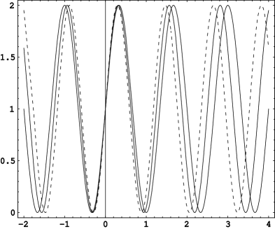
Optical pathlength difference, $x$

Fringe amplitude

Fringe amplitude

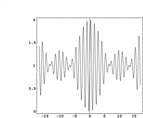
Optical pathlength difference, $x$

Fig. 6: Shown on the left are three monochromatic waves within the narrow finite bandwidth. Right plot shows interference of the polychromatic light that was composed as a superposition of these three waves. Note the envelope correction to the fringe visibility as a function of the OPD.

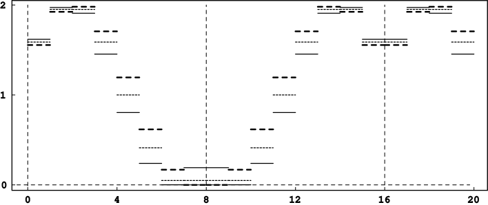
Optical pathlength difference, [bins]

Fringe amplitude

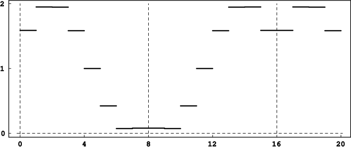
Optical pathlength difference, [bins]

Fringe amplitude

Fig. 7: Upper plot shows typical behavior of three monochromatic sinusoidal fringes modulated in 8 equal steps over a wavelength (as shown in upper plot of Figure 4). Parameters for the waves are given as $\phi=k_{i}x$, $\phi_{0}=0$, with $k_{1}=0.75k_{0}$ (thick dashed line), $k_{2}=0.8k_{0}$ (thin dashed line), $k_{3}=0.85k_{0}$ (thin solid line), thus the width of the spectral channel is $\Delta k=0.1k_{0}$. Lower plot shows polychromatic fringe composed from these three waves.

The integration over time may be performed in a general form and corresponding expression for the photon count, $N_{\ell i}$, is given as follows:

$$N_{\ell i} = {\cal I}_{0\ell}\bigg{(}1\,+V_{0\ell}\sin\phi(k_{\ell})\,{\sf Re}\big{\{}{\tilde{\cal P}}_{\ell i}\big{\}}+V_{0\ell}\cos\phi(k_{\ell})\,{\sf Im}\big{\{}{\tilde{\cal P}}_{\ell i}\big{\}}\bigg{)},$$ (51)

with quantities ${\sf Re}\big{\{}{\tilde{\cal P}}_{\ell i}\big{\}}$ and ${\sf Im}\big{\{}{\tilde{\cal P}}_{\ell i}\big{\}}$ given as below:

$${\sf Re}\big{\{}{\tilde{\cal P}}_{\ell i}\big{\}} = \frac{1}{\Delta\tau_{i}}\int_{t^{-}_{i}}^{t^{+}_{i}}\!\!{\cal E}_{\ell}\big{[}\Delta k_{\ell},\phi(k_{\ell}),x(t)\big{]}\cos\big{[}k_{\ell}x(t)+\Omega_{\ell}[\Delta k_{\ell},\phi(k_{\ell}),x(t)]\,\big{]}dt,$$

$${\sf Im}\big{\{}{\tilde{\cal P}}_{\ell i}\big{\}} = \frac{1}{\Delta\tau_{i}}\int_{t^{-}_{i}}^{t^{+}_{i}}\!\!{\cal E}_{\ell}\big{[}\Delta k_{\ell},\phi(k_{\ell}),x(t)\big{]}\sin\big{[}k_{\ell}x(t)+\Omega_{\ell}[\Delta k_{\ell},\phi(k_{\ell}),x(t)]\,\big{]}dt.\hskip 20.0pt$$ (52)

For convenience of further analysis, we combined these two real-valued matrices into one complex matrix ${\tilde{\cal P}}_{\ell i}$

$${\tilde{\cal P}}_{\ell i} = {\sf Re}\big{\{}{\tilde{\cal P}}_{\ell i}\big{\}}+j\,\,{\sf Im}\big{\{}{\tilde{\cal P}}_{\ell i}\big{\}}.$$ (53)

Furthermore, with definitions for ${\sf Re}\big{\{}{\tilde{\cal P}}_{\ell i}\big{\}}$ and ${\sf Im}\big{\{}{\tilde{\cal P}}_{\ell i}\big{\}}$, Eq. (52), this complex matrix may be presented as given below

$${\tilde{\cal P}}_{\ell i} = \frac{1}{\Delta\tau_{i}}\int_{t^{-}_{i}}^{t^{+}_{i}}\!\!{\cal E}_{\ell}\big{[}\Delta k_{\ell},\phi(k_{\ell}),x(t)\big{]}e^{j\,\big{(}k_{\ell}x(t)+\Omega_{\ell}[\Delta k_{\ell},\phi(k_{\ell}),x(t)]\,\big{)}}dt,$$ (54)

which, with the help of Eq. (44), is conveniently transforms as follows

$${\tilde{\cal P}}_{\ell i} = \frac{1}{\Delta\tau_{i}}\int_{t^{-}_{i}}^{t^{+}_{i}}\!\!e^{j\,k_{\ell}x(t)}\,\,{\tilde{W}_{\ell}}\big{[}\Delta k_{\ell},\phi(k_{\ell}),x(t)\big{]}dt,$$ (55)

where the complex envelope function ${\tilde{W}_{\ell}}$ given by Eqs. (39)-(40).

Eq. (55) may further be transformed to establish its true dependency of the integrand on time and wavenumber. To do this, we substitute expression for complex envelope function, Eq. (40), directly into Eq. (55) and obtain the following form for matrix ${\tilde{\cal P}}_{\ell i}$ with explicit dependency of the integrand:

$${\tilde{\cal P}}_{\ell i} = \frac{1}{{\cal I}_{0\ell}V_{0\ell}\Delta k_{\ell}\Delta\tau_{i}}\int_{t^{-}_{i}}^{t^{+}_{i}}\!\!\int_{k^{-}_{\ell}}^{k^{+}_{\ell}}\!\!{\cal F}(k){\cal I}_{0}(k)V(k)\,e^{j\,\big{(}k\,x(t)+\phi(k)-\phi(k_{\ell})\big{)}}dtdk.$$ (56)

Finally, we have defined everything that is needed to study Eq. (51), for the polychromatic fringe, which may equivalently be presented in a matrix form as below

$$\begin{array}[]{(}{c})N_{\ell 1}\\[0.0pt] ...\\[0.0pt] N_{\ell N}\end{array} = \begin{array}[]{(}{ccc})1;&~{}{\sf Im}\big{\{}{\tilde{\cal P}}_{\ell 1}\big{\}};&~{}{\sf Re}\big{\{}{\tilde{\cal P}}_{\ell 1}\big{\}}\\[0.0pt] ...&...&...\\[0.0pt] 1;&~{}{\sf Im}\big{\{}{\tilde{\cal P}}_{\ell N}\big{\}};&~{}{\sf Re}\big{\{}{\tilde{\cal P}}_{\ell N}\big{\}}\end{array}\begin{array}[]{(}{c}){\cal I}_{0\ell}\\[0.0pt] {\cal I}_{0\ell}V_{0\ell}\cos\phi(k_{\ell})\\[0.0pt] {\cal I}_{0\ell}V_{0\ell}\sin\phi(k_{\ell})\end{array},$$ (66)

where the complex matrix ${\tilde{\cal P}}_{\ell i}$ is given by Eq. (56).

The obtained result Eq. (51), (56) (or, equivalently Eq. (66)) constitutes the general form of expression for the polychromatic fringe. We will use this result to finalize the development of the general from of the observational model for polychromatic case with arbitrary phase modulation.

Ideally, one would need to determine not only three quantities ${\cal I}_{0\ell}V_{0\ell}\cos\phi(k_{\ell})$, ${\cal I}_{0\ell}V_{0\ell}\sin(k_{\ell}),$ and ${\cal I}_{0\ell}$, but the full functional dependency of the original quantities. However, the finite width of the observational band-width $\Delta k_{\ell}$ complicates the estimation process by bringing the non-linearity in the observational equation via the envelop function $W$. Note that if one neglects the size of the bandwidth $\Delta k_{\ell}$ with respect to the mean wavenumber $k_{\ell}$ or $\Delta k_{\ell}/{k_{\ell}}\rightarrow 0$ (the envelop function becomes unity $W\rightarrow 1$), one recovers the full simplicity of the monochromatic case represented by Eq. (6).[3]

4 General Solution for Polychromatic Phasors With Noisy Data

Currently in use, there are two fringe estimators, one for visibility (the unbiased estimator is $V^{2}$), and one for the phase (the unbiased estimator is the complex phasor). The $V^{2}$ estimator is already worked out in much detail (i.e. Refs. 4,10-13) if the complex phasor estimator is completed. So the development of the complex phasor was the main purpose for the presented work. As it is known, the complex fringe visibility can be represented by a phasor; if the fringe is stable, we can add the phasors vectorially over multiple samples. This co-adding can provide an improved signal-to-noise ratio. To co-add the fringe phasors requires a phase reference, for instance the white light phase.[7, 8]

In this Section we will develop optimally-weighted solution that accounts for a number of noise sources and will be applicable for a general case of delay modulation.

A Fringe Equation for Noisy Data

For the purposes of clarity we will omit spectral index $\ell$. All the obtained results are valid for any channel and thus could be easily reconstructed, if needed.

In the case of noisy data, observations of photon-counts $N_{i}$ are actually done with errors and, in reality, we observe $N_{i}={\bar{N}}_{i}+\epsilon_{i}$, where ${\bar{N}}_{i}$ is the value of photon counts at the $i$-th temporal bin in the absence of noise and $\epsilon_{i}$ is a random variable, representing the noise contribution to the measurements. We assume that $\epsilon_{i}$ are random variables that are primarily due to gaussian statistics. (This approach may be extended to incorporate other sources of noise.[19] The corresponding results will be reported elsewhere.) that are distributed around zero and following relations are valid

$$N_{i}={\bar{N}}_{i}+\epsilon_{i},\qquad\qquad E(\epsilon_{i})=0,\qquad\qquad E(\epsilon_{i}^{2})=\sigma_{i}^{2}.$$ (67)

In the general case one must account not only for the Gaussian statistics of read-out process, but also for the Poisson statistic that governs photo-emission (and photo-counting) process. Thus, a correct approach would be to assume that $\epsilon_{i}$ is a sum of two terms $\epsilon_{i}=\mu\,\epsilon^{G}_{i}+(1-\mu)\,\epsilon^{P}_{i}$, where $\epsilon^{G}_{i}$ is Gaussian and $\epsilon^{P}_{i}$ is Poissonian variables and $\mu$ is a number between 0 and 1. Expected complication arises from the fact that standard deviation computed for the photon-counting Poissonian bias is actually proportional to the signal ${(\sigma^{P}_{i})}^{2}\propto{\bar{\cal I}}_{i}$ (see discussion in Ref. 10). This issue is out of scope of the present paper and we will address this issue at a later time.

We also assume that $N_{i}$ are independent, therefore, we may form a diagonal covariance matrix for the quantities $N_{i}$ (or equivalently for $\epsilon_{i}$) with dispersions $\sigma_{i}^{2}$ on the diagonal:

$$C_{y}=\begin{array}[]{(}{cccc})\sigma_{1}^{2};&0;&...&0\\ 0;&\sigma_{2}^{2};&...&0\\ ...&...&...&0\\ 0;&0;&...&\sigma_{N}^{2}\end{array},\qquad G_{y}=C^{-1}_{y}=\begin{array}[]{(}{cccc})\sigma_{1}^{-2};&0;&...&0\\ 0;&\sigma_{2}^{-2};&...&0\\ ...&...&...&0\\ 0;&0;&...&\sigma_{N}^{-2}\end{array},$$ (68)

where $G_{y}$ is the matrix of weights. Therefore, in the case when noise is present in the data, equation (51) has following matrix form as below

$${\bar{N}}_{i}+\epsilon_{i} = \Big{(}1;~{}~{}{\sf Im}\big{\{}{\tilde{\cal P}}_{\ell i}\big{\}};~{}~{}{\sf Re}\big{\{}{\tilde{\cal P}}_{\ell i}\big{\}}\Big{)}\begin{array}[]{(}{c}){\cal I}_{0\ell}\\[0.0pt] {\cal I}_{0\ell}V_{0\ell}\cos\phi(k_{\ell})\\[0.0pt] {\cal I}_{0\ell}V_{0\ell}\sin\phi(k_{\ell})\end{array},$$ (72)

or, equivalently,

$${\bar{N}}_{i}+\epsilon_{i}=A_{i\alpha}X^{\alpha},$$ (73)

with indexes $i$ and $\alpha$ running as $i\in\{1,...,N\}$ and $\alpha\in\{1,2,3\}$. Vector $X^{\alpha}\equiv\Big{(}{\cal I}_{0\ell};\,{\cal I}_{0\ell}V_{0\ell}\cos\phi(k_{\ell});\,{\cal I}_{0\ell}V_{0\ell}\sin\phi(k_{\ell})\Big{)}^{T}$ is the vector to be determined and matrix ${\bf A}^{T}=A_{i\alpha}\equiv\big{(}1;{\sf Im}\big{\{}{\tilde{\cal P}}_{\ell i}\big{\}};{\sf Re}\big{\{}{\tilde{\cal P}}_{\ell i}\big{\}}\big{)}$ is the $3\times N$ rotational matrix in the phase space. A maximum likelihood solution to the system of equations (73) may be given by the following system of equations

$$X^{\alpha}=\sum_{i}^{N}{{\bf A}^{\dagger}_{\diamond}}^{i\alpha}{\bar{N}}_{i},\qquad\qquad{\rm where}\qquad\qquad{{\bf A}^{\dagger}_{\diamond}}=({\bf A}^{T}G_{y}{\bf A})^{-1}{\bf A}^{T}G_{y},$$ (74)

with ${{\bf A}^{\dagger}_{\diamond}}$ being an optimally-weighted pseudo-inverse matrix. Note that by choosing different gain matrix[4] instead of optimally weighted least-squared matrix Eq. (68), one may obtain solution with different, specifically designed properties. Nevertheless, our solution has enough embedded generality as it allows for arbitrary properties of noise contribution, which will be further explored below.

B Optimally-Weighted Pseudo-Inverse Matrix

In this Section we will find solution for the pseudo-inverse matrix ${{\bf A}^{\dagger}_{\diamond}}$ that was introduced by Eq.(74). To construct this matrix we will use the weights matrix $G_{y}$ given by Eq.(68) and the rotation matrix ${\bf A}_{\diamond}$ given by Eq.(55) as:

$${\bf A}_{i} = \Big{(}1;~{}\,{\sf Im}\big{\{}{\tilde{\cal P}}_{i}\big{\}};~{}{\sf Re}\big{\{}{\tilde{\cal P}}_{i}\big{\}}\Big{)}\equiv\Big{(}1;~{}s_{i};~{}c_{i}\Big{)},$$ (75)

where we denoted $s_{i}={\sf Im}\big{\{}{\tilde{\cal P}}_{i}\big{\}},c_{i}={\sf Re}\big{\{}{\tilde{\cal P}}_{i}\big{\}}$.

Let us construct matrix $({\bf A}^{T}G_{y}{\bf A})$ first. Calculation of $({\bf A}^{T}G_{y}{\bf A})$ is straightforward even for the most general case of arbitrary number of temporal bins ($N\geq 3$) and with arbitrary integration intervals ($\Delta\tau_{i}\not=\Delta\tau_{j}$ for $i\not=j$). Thus, after some algebra we find the following structure:

$$({\bf A}^{T}G_{y})=\begin{array}[]{(}{c})\frac{1}{\sigma_{1}^{2}};~{}\frac{1}{\sigma_{2}^{2}};~{}...~{}\frac{1}{\sigma_{N}^{2}}\\[0.0pt] \frac{s_{1}}{\sigma_{1}^{2}};~{}\frac{s_{2}}{\sigma_{2}^{2}};~{}...~{}\frac{s_{N}}{\sigma_{N}^{2}}\\[0.0pt] \frac{c_{1}}{\sigma_{1}^{2}};~{}\frac{c_{2}}{\sigma_{2}^{2}};~{}...~{}\frac{c_{N}}{\sigma_{N}^{2}}\end{array},~{}~{}({\bf A}^{T}G_{y}{\bf A})~{}=~{}\begin{array}[]{(}{lll})\overset{N}{\underset{i}{\sum}}\frac{1}{\sigma_{i}^{2}}&\overset{N}{\underset{i}{\sum}}\frac{s_{i}}{\sigma_{i}^{2}}&\overset{N}{\underset{i}{\sum}}\frac{c_{i}}{\sigma_{i}^{2}}\\[0.0pt] \overset{N}{\underset{i}{\sum}}\frac{s_{i}}{\sigma_{i}^{2}}&\overset{N}{\underset{i}{\sum}}\frac{s_{i}^{2}}{\sigma_{i}^{2}}&\overset{N}{\underset{i}{\sum}}\frac{s_{i}c_{i}}{\sigma_{i}^{2}}\\[0.0pt] \overset{N}{\underset{i}{\sum}}\frac{c_{i}}{\sigma_{i}^{2}}&\overset{N}{\underset{i}{\sum}}\frac{s_{i}c_{i}}{\sigma_{i}^{2}}&\overset{N}{\underset{i}{\sum}}\frac{c_{i}^{2}}{\sigma_{i}^{2}}\\ \end{array}.$$ (76)

By inverting the obtained result one constructs the covariance matrix $\Lambda$ of the following structure:

$$\hskip 20.0pt{\bf\Lambda}~{}=~{}({\bf A}^{T}G_{y}{\bf A})^{-1}~{}=$$

$$\hskip-30.0pt=~{}\frac{1}{\Delta_{\diamond}}\begin{array}[]{(}{lll})~{}~{}\,\frac{1}{2}\overset{N}{\underset{ij}{\sum}}\frac{(s_{i}c_{j}-c_{i}s_{j})^{2}}{\sigma_{i}^{2}\sigma_{j}^{2}}&~{}~{}\frac{1}{2}\overset{N}{\underset{ij}{\sum}}\frac{(c_{i}-c_{j})(s_{i}c_{j}-c_{i}s_{j})}{\sigma_{i}^{2}\sigma_{j}^{2}}&-\frac{1}{2}\overset{N}{\underset{ij}{\sum}}\frac{(s_{i}-s_{j})(s_{i}c_{j}-c_{i}s_{j})}{\sigma_{i}^{2}\sigma_{j}^{2}}\\[10.0pt] ~{}~{}\frac{1}{2}\overset{N}{\underset{ij}{\sum}}\frac{(c_{i}-c_{j})(s_{i}c_{j}-c_{i}s_{j})}{\sigma_{i}^{2}\sigma_{j}^{2}}&~{}~{}\frac{1}{2}\overset{N}{\underset{ij}{\sum}}\frac{(c_{i}-c_{j})^{2}}{\sigma_{i}^{2}\sigma_{j}^{2}}&-\frac{1}{2}\overset{N}{\underset{ij}{\sum}}\frac{(s_{i}-s_{j})(c_{i}-c_{j})}{\sigma_{i}^{2}\sigma_{j}^{2}}\\[0.0pt] -\frac{1}{2}\overset{N}{\underset{ij}{\sum}}\frac{(s_{i}-s_{j})(s_{i}c_{j}-c_{i}s_{j})}{\sigma_{i}^{2}\sigma_{j}^{2}}&-\frac{1}{2}\overset{N}{\underset{ij}{\sum}}\frac{(s_{i}-s_{j})(c_{i}-c_{j})}{\sigma_{i}^{2}\sigma_{j}^{2}}&~{}~{}\,\frac{1}{2}\overset{N}{\underset{ij}{\sum}}\frac{(s_{i}-s_{j})^{2}}{\sigma_{i}^{2}\sigma_{j}^{2}}\end{array},$$

where determinant of the matrix $({\bf A}^{T}G_{y}{\bf A})$, $\Delta_{\diamond}=\det||({\bf A}^{T}G_{y}{\bf A})||$, is given as

$$\Delta_{\diamond} = \frac{1}{2}\overset{N}{\underset{ijk}{\sum}}~{}\frac{(s_{i}c_{j}-s_{j}c_{i})}{\sigma_{i}^{2}\sigma_{j}^{2}\sigma_{k}^{2}}\Big{[}(s_{i}c_{j}-s_{j}c_{i})+(s_{j}c_{k}-s_{k}c_{j})+(s_{k}c_{i}-s_{i}c_{k})\Big{]},$$ (80)

with a triple summation for all the indexes denoting the temporal bins and running from 1 to $N$, namely $\forall~{}~{}\{i,j,k\}\in[1,...,N]$.

These intermediate results allow us to write the solution for the $(N\times 3)$ optimally-weighted pseudo-inverse matrix ${{\bf A}^{\dagger}_{\diamond}}={A_{\diamond}^{\dagger}}^{\alpha}_{k}$ in the following compact form:

$${{\bf A}^{\dagger}_{\diamond}}=({\bf A}^{T}G_{y}{\bf A})^{-1}{\bf A}^{T}G_{y}=\frac{1}{{\cal D}^{\diamond}}\begin{array}[]{(}{c}){\cal A}^{\diamond}_{k}\\[-2.0pt] {\cal B}^{\diamond}_{k}\\[-2.0pt] {\cal C}^{\diamond}_{k}\end{array},$$ (81)

where coefficients ${\cal A}^{\diamond}_{k},{\cal B}^{\diamond}_{k},{\cal C}^{\diamond}_{k}$ and ${\cal D}^{\diamond}$ depend on duration of each temporal bin, mean wavenumber and variances for the data taken in each bin, and are given by

$${\cal A}_{k}^{\diamond} = {\overset{N}{\underset{ij}{\sum}}~{}\frac{1}{\sigma_{i}^{2}\sigma_{j}^{2}\sigma_{k}^{2}}\big{(}s_{i}c_{j}-s_{j}c_{i}\big{)}\big{[}(s_{i}c_{j}-s_{j}c_{i})+(s_{j}c_{k}-s_{k}c_{j})+(s_{k}c_{i}-s_{i}c_{k})\big{]}},$$

$${\cal B}_{k}^{\diamond} = {\overset{N}{\underset{ij}{\sum}}~{}\frac{1}{\sigma_{i}^{2}\sigma_{j}^{2}\sigma_{k}^{2}}\big{(}c_{i}-c_{j}\big{)}~{}\big{[}(s_{i}c_{j}-s_{j}c_{i})+(s_{j}c_{k}-s_{k}c_{j})+(s_{k}c_{i}-s_{i}c_{k})\big{]}},$$

$${\cal C}_{k}^{\diamond} = -~{}{\overset{N}{\underset{ij}{\sum}}~{}\frac{1}{\sigma_{i}^{2}\sigma_{j}^{2}\sigma_{k}^{2}}\big{(}s_{i}-s_{j}\big{)}~{}\big{[}(s_{i}c_{j}-s_{j}c_{i})+(s_{j}c_{k}-s_{k}c_{j})+(s_{k}c_{i}-s_{i}c_{k})\big{]}},$$

$${\cal D}^{\diamond} = \overset{N}{\underset{k}{\sum}}~{}{\cal A}^{\diamond}_{k}~{}=~{}\frac{1}{3}\overset{N}{\underset{ijk}{\sum}}\frac{1}{\sigma_{i}^{2}\sigma_{j}^{2}\sigma_{k}^{2}}\big{[}(s_{i}c_{j}-s_{j}c_{i})+(s_{j}c_{k}-s_{k}c_{j})+(s_{k}c_{i}-s_{i}c_{k})\big{]}^{2}.\hskip 20.0pt$$ (82)

Definitions for the quantities $s_{i}$ and $c_{i}$, $s_{i}={\sf Im}\big{\{}{\tilde{\cal P}}_{i}\big{\}},c_{i}={\sf Re}\big{\{}{\tilde{\cal P}}_{i}\big{\}}$, allow to present expressions (82) in a more convenient form. First, remember that complex matrix, ${\tilde{\cal P}}_{i}$, as any complex function, may be represented by its amplitude and its phase, namely

$${\tilde{\cal P}}_{i} = {\sf Re}\big{\{}{\tilde{\cal P}}_{i}\big{\}}+j\,\,{\sf Im}\big{\{}{\tilde{\cal P}}_{i}\big{\}}=p_{i}\,e^{j\pi_{i}},$$ (83)

where $p_{i}$ and $\pi_{i}$ are the amplitude and the phase of this complex matrix correspondingly and are given as follows:

$$p_{i}=\sqrt{{\sf Re}^{2}\big{\{}{\tilde{\cal P}}_{i}\big{\}}+{\sf Im}^{2}\big{\{}{\tilde{\cal P}}_{i}\big{\}}},\qquad\pi_{i}={\sf ArcTan}\Big{\{}\frac{{\sf Im}\big{\{}{\tilde{\cal P}}_{i}\big{\}}}{{\sf Re}\big{\{}{\tilde{\cal P}}_{i}\big{\}}}\Big{\}},$$ (84)

with complex matrix ${\tilde{\cal P}}_{\ell i}$ is given by Eq. (55). These quantities allow presentation of Eqs. (82) in the following form:

$${\cal A}_{k}^{\diamond} = \overset{N}{\underset{ij}{\sum}}~{}\frac{p_{i}p_{j}\sin[\pi_{i}-\pi_{j}]}{\sigma_{i}^{2}\sigma_{j}^{2}\sigma_{k}^{2}}\times$$

$$\hskip 25.0pt\times\Big{(}p_{i}p_{j}\sin[\pi_{i}-\pi_{j}]+p_{j}p_{k}\sin[\pi_{j}-\pi_{k}]+p_{k}p_{i}\,\sin[\pi_{k}-\pi_{i}]\Big{)},$$

$${\cal B}_{k}^{\diamond} = \overset{N}{\underset{ij}{\sum}}~{}\frac{\big{(}p_{i}\cos\pi_{i}-p_{j}\cos\pi_{j}\big{)}}{\sigma_{i}^{2}\sigma_{j}^{2}\sigma_{k}^{2}}\times$$

$$\hskip 25.0pt\times\Big{(}p_{i}p_{j}\sin[\pi_{i}-\pi_{j}]+p_{j}p_{k}\sin[\pi_{j}-\pi_{k}]+p_{k}p_{i}\sin[\pi_{k}-\pi_{i}]\Big{)},$$

$${\cal C}_{k}^{\diamond} = -~{}\overset{N}{\underset{ij}{\sum}}~{}\frac{\big{(}p_{i}\sin\pi_{i}-p_{j}\sin\pi_{j}\big{)}}{\sigma_{i}^{2}\sigma_{j}^{2}\sigma_{k}^{2}}\times$$

$$\hskip 25.0pt\times\Big{(}p_{i}p_{j}\sin[\pi_{i}-\pi_{j}]+p_{j}p_{k}\,\sin[\pi_{j}-\pi_{k}]+p_{k}p_{i}\,\sin[\pi_{k}-\pi_{i}]\Big{)},$$

$${\cal D}^{\diamond} = \overset{N}{\underset{k}{\sum}}~{}{\cal A}^{\diamond}_{k}=$$ (85)

$$= \frac{1}{3}\overset{N}{\underset{ijk}{\sum}}\frac{1}{\sigma_{i}^{2}\sigma_{j}^{2}\sigma_{k}^{2}}\Big{(}p_{i}p_{j}\sin[\pi_{i}-\pi_{j}]+p_{j}p_{k}\sin[\pi_{j}-\pi_{k}]+p_{k}p_{i}\sin[\pi_{k}-\pi_{i}]\Big{)}^{2}.\hskip 10.0pt$$

At this point we have all the expressions necessary to present the optimally-weighted solution for the polychromatic phasors.

C Photon Noise-Optimized Solution for Polychromatic Phasors

An optimally-weighted solution for the quantities $X^{\alpha}$ may be obtained directly now from Eq.(74) with the help of expressions (81)-(82) in the following compact form:

$${\cal I}^{\diamond}_{0} = \frac{1}{{\cal D}^{\diamond}}\overset{N}{\underset{k}{\sum}}~{}{\bar{N}}_{k}~{}{\cal A}^{\diamond}_{k},$$

$${\cal I}^{\diamond}_{0}~{}V_{0}^{\diamond}\cos\bar{\phi}^{\diamond} = \frac{1}{{\cal D}^{\diamond}}\overset{N}{\underset{k}{\sum}}~{}{\bar{N}}_{k}~{}{\cal B}^{\diamond}_{k},$$

$${\cal I}^{\diamond}_{0}~{}V_{0}^{\diamond}\sin\bar{\phi}^{\diamond} = \frac{1}{{\cal D}^{\diamond}}\overset{N}{\underset{k}{\sum}}~{}{\bar{N}}_{k}~{}{\cal C}^{\diamond}_{k}.$$ (86)

with coefficients of ${\cal A}^{\diamond}_{k},{\cal B}^{\diamond}_{k},{\cal C}^{\diamond}_{k}$ and ${\cal D}^{\diamond}$ are given by Eqs.(82) and (85).

The obtained solution for the polychromatic visibility phasors given by Eq. (86) is given in the form of a linear combination of weighted photon counts recorded during a particular integration period. This form turned out to be very helpful when analyzing contributions of CCD pixels that are systematically biased. The obtained result may be used to de-weight ’bad’ pixels (in a statistical sense) and, thus, to reduce the problem of biases while estimating fringe parameters.

This form allows to express an optimally-weighted solution for visibility, phase and the constant intensity terms in a familiar compact form:

$${V^{\diamond}_{0}}^{2} = \frac{\big{(}\overset{N}{\underset{k}{\sum}}~{}{\bar{N}}_{k}\,{\cal B}^{\diamond}_{k}\big{)}^{2}+\big{(}\overset{N}{\underset{k}{\sum}}~{}{\bar{N}}_{k}\,{\cal C}^{\diamond}_{k}\big{)}^{2}}{\big{(}\overset{N}{\underset{k}{\sum}}~{}{\bar{N}}_{k}\,{\cal A}^{\diamond}_{k}\big{)}^{2}},$$

$$\bar{\phi}^{\diamond} = \text{ArcTan}\Big{[}\,\frac{\overset{N}{\underset{k}{\sum}}~{}{\bar{N}}_{k}~{}{\cal C}^{\diamond}_{k}}{\overset{N}{\underset{k}{\sum}}~{}{\bar{N}}_{k}~{}{\cal B}^{\diamond}_{k}}\,\Big{]},\qquad~{}~{}{\cal I}^{\diamond}_{0}=\frac{\overset{N}{\underset{k}{\sum}}~{}{\bar{N}}_{k}~{}{\cal A}^{\diamond}_{k}}{\overset{N}{\underset{k}{\sum}}~{}{\cal A}^{\diamond}_{k}}.$$ (87)

The form of the obtained solution is simple to understand and it is straightforward to implement in the software codes. All the information necessary to calculate the $3N$ coefficients of ${\cal A}^{\diamond}_{k},{\cal B}^{\diamond}_{k},{\cal C}^{\diamond}_{k}$ and ${\cal D}^{\diamond}$ is presumed to be known before the experiment. Thus, for the case when $N=8$ one would have to calculate only 24 numbers from Eq. (82). These numbers correspond to 8 numbers of ${\cal A}^{\diamond}_{k}$, 8 numbers of ${\cal B}^{\diamond}_{k}$ and 8 numbers of ${\cal C}^{\diamond}_{k}$. The experimental data is used as input to Eqs. (86) (or directly Eqs. (87)) to produce the best estimates of the actual values for visibility, phase and the constant intensity term. This approach is currently being utilized and corresponding results will be reported elsewhere.

5 Filtered Polychromatic Light: Spectral Channels with Narrow Bands

It is thought now that SIM will be operating at 80 spectral channels for the science interferometer and at 4 channels for both guide interferometers. The data will be read at a millisecond time rate. SIM will be dispersing light just before the interfering radiation reaches the detector. To take this fact into account, we define a filter that allows to limit the total bandwidth of the incoming radiation. We will formally denote a filter with such a properties as follows:

$${\cal F}_{\ell}(k)={\cal F}_{\ell}(k-k_{\ell};\Delta k_{\ell}).$$ (88)

We assumed that this filter operates within the ${\ell}$-th spectral channel by allowing to pass through only such a radiation that is composed from the frequencies corresponding to the mean (or central) wavenumber $k_{\ell}$ within the bandwidth of $\Delta k_{\ell}$. Thus, filter ${\cal F}_{\ell}(k)$ enables the instrument to “see” light only in a certain interval $\Delta k_{\ell}$ around the mean number $k_{\ell}$.

In this Section we will develop a model that employes such an approach for the case of a rectangular bandpass filter. Due to its analytical simplicity, the rectangular bandpass filter is the most known construction in the Fourier optics. This analysis will allow us to establish correspondence with the previously obtained results both for monochromatic and polychromatic light.

A Rectangular Bandpass Filter

To take advantage of the results derived in the previous section, we must first decide on the properties of the bandpass filter. This decision in return will affect the properties of the envelop function. Below we shall develop a model for a special case of the bandpass filter – a rectangular bandpass filter denoted here as ${\cal F}_{\ell}$, which is done analytically in the following form

$${\cal F}(k)=\sum_{\ell=1}^{L}{\cal F}_{\ell}(k),\qquad{\rm where}\qquad{\cal F}_{\ell}(k)=\begin{cases}~{}~{}{{\cal F}_{0\ell}}\,=\,{\rm const},&~{}~{}~{}~{}\text{ $k\in[k^{-}_{\ell},k^{+}_{\ell}]$},\\[-10.0pt] ~{}~{}~{}~{}0,&~{}~{}~{}~{}\text{ $k\not\in[k^{-}_{\ell},k^{+}_{\ell}]$}.\end{cases}$$ (89)

We can also assume that the width of a spectral channel is small, so that both intensity of incoming radiation, ${\cal I}_{0}(k)$, and apparent visibility, $V(k)$, do not change within the spectral channel (in particular, this leads to $\hat{V}_{0\ell}(k)\equiv 1$ in Eqs. (32) and (33)). Therefore, the following conditions are satisfied with a particular spectral channel, $\ell$:

$${\cal I}_{0}(k)={\rm const},\qquad V(k) = {\rm const},\qquad{\cal F}_{0\ell}={\rm const},$$ (90)

$$\phi(k)-\phi(k_{\ell}) = d_{0\ell}(k-k_{\ell})+{\cal O}(\frac{\partial^{2}\phi}{\partial k_{\ell}^{2}}),$$ (91)

where $d_{0\ell}=\frac{\partial\phi}{\partial k_{\ell}}$ is the delay within the $\ell$-th channel.

One may perform integration of the fringe envelope function ${\tilde{W}_{\ell}}\big{[}x(t)\big{]}$ which is given by Eq. (39) (or use equation (133) for the unperturbed envelope function and then apply iterative procedure outlined in Appendix B.). To the second order in phase variation (i.e. ${\cal O}(\frac{\partial^{2}\phi}{\partial k_{\ell}^{2}})$), the resulted envelope function has following properties:

$${\tilde{W}_{\ell}}\big{[}\Delta k_{\ell},\phi(k_{\ell}),x_{i}\big{]} = \frac{1}{{\cal I}_{0\ell}V_{0\ell}\Delta k_{\ell}}\int_{k^{-}_{\ell}}^{k^{+}_{\ell}}\!\!{\cal F}(k){\cal I}_{0}(k)V(k)\,e^{j\,\big{(}(k-k_{\ell})x(t)+\phi(k)-\phi(k_{\ell})\big{)}}dk=$$ (92)

$$= \frac{1}{\Delta k_{\ell}}\int_{k^{-}_{\ell}}^{k^{+}_{\ell}}\!\!e^{j\,(k-k_{\ell})\big{(}x(t)\,+\,d_{0\ell}\big{)}}dk+{\cal O}(\frac{\partial^{2}\phi}{\partial k_{\ell}^{2}}).$$

Let us introduce a convenient variable, $\kappa=k-k_{\ell}$, and remember that $\Delta k_{\ell}=k^{+}_{\ell}-k^{-}_{\ell}$ and $k_{\ell}=\frac{1}{2}(k^{+}_{\ell}+k^{-}_{\ell})$ are the width of the spectral channel and the mean wavenumber. This allows us to integrate expression (92) over the wavenumber space

$${\tilde{W}_{\ell}}\big{[}\Delta k_{\ell},\phi(k_{\ell}),x_{i}\big{]} = \frac{1}{\Delta k_{\ell}}\int_{-\frac{1}{2}\Delta k_{\ell}}^{+\frac{1}{2}\Delta k_{\ell}}\!\!e^{j\,\kappa\big{(}d_{0\ell}+x(t)\big{)}\!}d\kappa=\frac{\sin[\frac{1}{2}\Delta k_{\ell}(d_{0\ell}+x(t))]}{\frac{1}{2}\Delta k_{\ell}(d_{0\ell}+x(t))}.\hskip 20.0pt$$ (93)

We can now present Eq. (55) for matrix ${\tilde{\cal P}}_{\ell i}$ as follows:

$${\tilde{\cal P}}_{\ell i} = \frac{1}{\Delta\tau_{i}}\int_{t^{-}_{i}}^{t^{+}_{i}}\!\!e^{j\,k_{\ell}x(t)}\,\frac{\sin[\frac{1}{2}\Delta k_{\ell}(d_{0\ell}+x(t))]}{\frac{1}{2}\Delta k_{\ell}(d_{0\ell}+x(t))}\,dt.$$ (94)

At this moment, we introduce another convenient variable, $\tau=t-t_{i}$. Analogously, $\Delta\tau_{i}=t^{+}_{i}-t^{-}_{i}$ and $t_{i}=\frac{1}{2}(t^{+}_{i}+t^{-}_{i})$ are the duration of the temporal integration within the $i$-th bin and the mean time for this bin correspondingly. This result is used to transform Eq. (94) as below:

$${\tilde{\cal P}}_{\ell i} = \!\!{e^{j\,k_{\ell}x(t_{i})}}~{}\delta{\tilde{\cal P}}_{\ell i},$$ (95)

with matrix coefficient $\delta{\tilde{\cal P}}_{\ell i}$ given by

$$\delta{\tilde{\cal P}}_{\ell i}=\frac{1}{\Delta\tau_{i}}\int_{-\frac{1}{2}\Delta\tau_{i}}^{+\frac{1}{2}\Delta\tau_{i}}\!\!e^{j\,k_{\ell}\big{(}x(t_{i}+\tau)-x(t_{i})\big{)}}\,\frac{\sin[\frac{1}{2}\Delta k_{\ell}\big{(}d_{0\ell}+x(t_{i}+\tau)\big{)}]}{\frac{1}{2}\Delta k_{\ell}\big{(}d_{0\ell}+x(t_{i}+\tau)\big{)}}\,d\tau.$$ (96)

The obtained result explicitly depends on the functional form of the OPD modulation, $x(t)$. To integrate this equation one first needs to make certain assumptions on the temporal behavior of $x(t)$, which will be done in the following Sections. At this moment we present Eq. (51) in the following form:

$$N_{\ell i} = {\cal I}_{0\ell}\bigg{(}1\,+V_{0\ell}\sin\big{[}\phi(k_{\ell})+k_{\ell}x(t_{i})\big{]}\,{\sf Re}\big{\{}\delta{\tilde{\cal P}}_{\ell i}\big{\}}+$$ (97)

$$\hskip 35.0pt+~{}V_{0\ell}\cos\big{[}\phi(k_{\ell})+k_{\ell}x(t_{i})\big{]}\,{\sf Im}\big{\{}\delta{\tilde{\cal P}}_{\ell i}\big{\}}\bigg{)},\hskip 10.0pt$$

where the complex matrix $\delta{\tilde{\cal P}}_{\ell i}$ is given by Eq. (96). The importance of separating terms with $\delta{\tilde{\cal P}}_{\ell i}$ is in the fact that one can establish clear correspondence with monochromatic light, for which $\delta{\tilde{\cal P}}_{\ell i}=I_{\ell i}$, the identity matrix.

In the next two subsections we will study two different special cases of OPD modulation, namely the stepping and ramping modulations of the optical path difference.

B Stepping Phase Modulation

The stepping phase modulation realized when the pathlength difference is changes as a set of discrete values corresponding to a number of steps in the OPD space. mathematically this process represented as follows:

$$x(t)=\sum_{i=1}^{N=8}x(t_{i}),~{}~{}~{}~{}~{}~{}\text{where}~{}~{}~{}~{}~{}~{}x(t_{i})=\begin{cases}x_{i},&~{}~{}~{}t~{}\in[t^{-}_{i},t_{i}^{+}],\\[-10.0pt] ~{}0,&~{}~{}~{}t~{}\not\in[t^{-}_{i},t_{i}^{+}],\end{cases}$$ (98)

with $t_{i}=\frac{1}{2}(t^{+}_{i}+t^{-}_{i})$. This procedure defines the temporal bins that will be used to modulate the interferometric pattern.

Conditions (98) allow for a significant simplification of temporal integration in Eq. (96). It simply is leading to a substitution $x(t)\rightarrow x_{i}$ in Eq. (43), and matrix ${\tilde{\cal P}}_{\ell i}$ takes the following form

$${\tilde{\cal P}}_{\ell i} = e^{j\,k_{\ell}x(t_{i})}\,\,\frac{\sin[\frac{1}{2}\Delta k_{\ell}\big{(}d_{0\ell}+x_{i}\big{)}]}{\frac{1}{2}\Delta k_{\ell}\big{(}d_{0\ell}+x_{i}\big{)}},$$ (99)

As a result, to the second order in the phase variation (i.e. $\phi(k_{\ell})\approx\phi_{\ell}+{\cal O}(\frac{\partial^{2}\phi}{\partial k_{\ell}^{2}}\Big{|}_{k_{\ell}})$), observational equation (97) is taking form as below:

$$N_{\ell i} = {\cal I}_{0\ell}\bigg{(}1+V_{0\ell}\,{\rm sinc}[\frac{1}{2}\Delta k_{\ell}\big{(}x_{i}+d_{0\ell}\big{)}]\,\sin\big{[}\phi(k_{\ell})+k_{\ell}x_{i}\big{]}\bigg{)}.$$ (100)

The obtained result Eq. (100) clearly depends on the particular form of the envelope function. As such, it has most of the parameters that are necessary for the phase estimation purposes in the case of wide bandwidth.

For the most practical cases the value of the ${sinc}$ function will be close to $\rm sinc\sim 1$. Indeed, let us analyze the argument of this function, $\frac{1}{2}\Delta k_{\ell}\big{(}x_{i}+d_{0\ell})$. Thus, one might expect that within the spectral channel the phase will stay constant, hence $d_{0\ell}=\frac{\partial\phi}{\partial k_{\ell}}\approx 0$. Furthermore, for the estimation purposes let us assume that all the step-sizes $x_{i}$ are essentially $x_{i}=i\frac{\lambda_{0}}{N}$, where $N$ is the total number of temporal integration bins, $i$ is the number of a particular temporal bin, $i\in[1,...,N]$, and $\lambda_{0}$ is the reference wavelength chosen for the OPD modulation (or $\lambda_{0}=\frac{2\pi}{k_{0}}$, where $k_{0}$ is the wavenumber corresponding to chosen modulation wavelength). Also remember that the width of a spectral channel is related to the total SIM bandwidth as $\Delta k_{\ell}=\frac{\Delta k_{\sf SIM}}{L}$, where $\Delta k_{\sf SIM}$ is the total SIM bandwidth and $L$ is the total number of spectral channels used for the white light fringe detection. Therefore, one has

$$\frac{1}{2}\Delta k_{\ell}\big{(}x_{i}+d_{0\ell})\approx\frac{1}{2}\Delta k_{\ell}x_{i}=\frac{\pi i}{LN}\frac{\Delta k_{\sf SIM}}{k_{0}}.$$ (101)

Assuming $\lambda_{\sf SIM}^{-}=450$ nm and $\lambda_{\sf SIM}^{+}=900$ nm, and $\lambda_{0}=900$ nm, thus yielding $\frac{\Delta k_{\sf SIM}}{k_{0}}=1.$ The maximal value for the expression (101) is realized when $i=N$, thus

$$\frac{\pi i}{LN}\frac{\Delta k_{\sf SIM}}{k_{0}}\leq\frac{\pi}{L}.$$ (102)

Currently, there are different numbers of spectral channels used to process data from our testbeds. This number may be as large as $L=80$ and as small as $L=4$. Of coarse, when $L=80$, the ratio $\pi/L$ becomes $\pi/L=0.03927$ and, thus, ${\sf sinc}[\frac{1}{2}\Delta k_{\ell}x_{i}]|_{L=80}=0.99974$, and similarly for $L=4$ the sinc function becomes ${\sf sinc}[\frac{1}{2}\Delta k_{\ell}x_{i}]|_{L=4}=0.90032$. We will address the issue of phase estimation sensitivity to the width of a spectral channel $\Delta k_{\ell}$ at a later time.

This observation allows us to present the sinc function as a series with respect to the small parameter ${\Delta k_{\ell}}z$ (with $z$ being defined as $z=x_{i}+d_{0\ell}$) as

$${\rm sinc}[\frac{\Delta k_{\ell}z}{2}] = \sum_{n=0}^{\infty}\frac{(-1)^{n}}{(2n+1)!}\big{[}\frac{\Delta k_{\ell}z}{2}\big{]}^{2n}$$ (103)

$$= 1-\frac{1}{3!}\big{[}\frac{\Delta k_{\ell}z}{2}\big{]}^{2}+\frac{1}{5!}\big{[}\frac{\Delta k_{\ell}z}{2}\big{]}^{4}+{\cal O}(\frac{1}{7!}\big{[}\frac{\Delta k_{\ell}z}{2}\big{]}^{6}),$$

one can present the expression Eq. (100) in the following form:

$$N_{\ell i} = {\cal I}_{0\ell}\Big{[}1+$$ (104)

$$+ V_{0\ell}\,\Big{(}1-\frac{\Delta k_{\ell}^{2}(x_{i}+d_{0\ell})^{2}}{24}+\frac{\Delta k_{\ell}^{4}(x_{i}+d_{0\ell})^{4}}{1920}\Big{)}\,\sin\big{[}\phi(k_{\ell})+k_{\ell}x_{i}\big{]}\Big{]}.$$

The obtained expression models the expected number of photons detected at the CCD for the rectangular bandpass filter and stepping phase modulation. It extends the results obtained for the monochromatic case on the finite size spectral bandwidth. This fact is indicated by the explicit dependency of the obtained result on the width of a spectral channel $\Delta k_{\ell}$. (For the most of the interesting practical applications, the size of the delay within a particular spectral channel is very small $d_{0\ell}=\frac{\partial\phi}{\partial k_{\ell}}\approx 0$, which further simplifies Eq. (104)).

C Ramping Phase Modulation

In this Section we will discuss another type of phase modulation – the case when the phase is linearly changes with time. This modulation utilizes the phase ramping technique.(For more details, see Refs.6-7.) To develop analytical solution we will be using the system equations developed above, specifically Eqs. (51) and (55).

The optical path difference for the case of ramping phase modulation is modeled as a continuous function of time as follows:

$$x(t)=x_{0}+v\,t,$$ (105)

where $x_{0}$ is the initial OPD value and $v$ is the instantaneous velocity of OPD modulation. Remembering the definition for $\tau$ as $\tau=t-t_{i}$, and $\Delta\tau_{i}=t^{+}_{i}-t^{-}_{i}$ and $t_{i}=\frac{1}{2}(t^{+}_{i}+t^{-}_{i})$, Eq. (96) takes the form:

$${\tilde{\cal P}}_{\ell i} = {e^{j\,k_{\ell}x(t_{i})}}\delta{\tilde{\cal P}}_{\ell i},$$ (106)

with coefficient $\delta{\tilde{\cal P}}_{\ell i}$ given by

$$\delta{\tilde{\cal P}}_{\ell i}=\frac{1}{\Delta\tau_{i}}\int_{-\frac{1}{2}\Delta\tau_{i}}^{+\frac{1}{2}\Delta\tau_{i}}\!\!e^{j\,k_{\ell}v\tau}\,\frac{\sin[\frac{1}{2}\Delta k_{\ell}z(\tau)]}{\frac{1}{2}\Delta k_{\ell}z(\tau)}\,d\tau$$ (107)

and $z(\tau)=d_{0\ell}+x(t_{i})+v\,\tau$. This allows us to present Eq. (97) in the following form:

$$N_{\ell i} = {\cal I}_{0\ell}\bigg{(}1+V_{0\ell}\sin\big{[}\phi(k_{\ell})+k_{\ell}x(t_{i})\big{]}\,{\sf Re}\big{\{}\delta{\tilde{\cal P}}_{\ell i}\big{\}}+$$ (108)

$$\hskip 31.0pt+~{}V_{0\ell}\cos\big{[}\phi(k_{\ell})+k_{\ell}x(t_{i})\big{]}\,{\sf Im}\big{\{}\delta{\tilde{\cal P}}_{\ell i}\big{\}}\bigg{)}\!,\hskip 10.0pt$$

where the complex matrix of additional rotation in the phase space, $\delta{\tilde{\cal P}}_{\ell i}$, is given by Eq. (96). Equation (108) may equivalently be presented in a matrix form as below

$$N_{\ell i} = \Big{(}1;~{}~{}\sin k_{\ell}x(t_{i});~{}~{}\cos k_{\ell}x(t_{i})\Big{)}\times$$ (115)

$$\hskip 30.0pt\times\begin{array}[]{(}{ccc})1&0&0\\[0.0pt] 0&~{}{\sf Re}\big{\{}\delta{\tilde{\cal P}}_{\ell i}\big{\}}&-{\sf Im}\big{\{}\delta{\tilde{\cal P}}_{\ell i}\big{\}}\\[0.0pt] 0&~{}{\sf Im}\big{\{}\delta{\tilde{\cal P}}_{\ell i}\big{\}};&~{}~{}{\sf Re}\big{\{}\delta{\tilde{\cal P}}_{\ell i}\big{\}}\end{array}\begin{array}[]{(}{c}){\cal I}_{0\ell}\\[0.0pt] {\cal I}_{0\ell}V_{0\ell}\cos\phi(k_{\ell})\\[0.0pt] {\cal I}_{0\ell}V_{0\ell}\sin\phi(k_{\ell})\end{array}.$$

The result of integration of Eq.(107) may not be presented in a compact analytical form. It rather could be expressed in the form of two functions defined as SinIntegral and CosIntegral. To simplify the analysis, the sinc function may be given in the form of power series expansion with respect to the small parameter $\Delta k_{\ell}z(\tau)$ as given by Eq. (103). This expansion allows us to present Eqs. (107) in the following form:

$$\delta{\tilde{\cal P}}_{\ell i} = \!\!\frac{1}{\Delta\tau_{i}}\int_{-\frac{1}{2}\Delta\tau_{i}}^{+\frac{1}{2}\Delta\tau_{i}}\!\!e^{j\,k_{\ell}v\tau}\,\frac{\sin[\frac{1}{2}\Delta k_{\ell}z(\tau)]}{\frac{1}{2}\Delta k_{\ell}z(\tau)}\,d\tau=$$ (116)

$$= \!\!\frac{1}{\Delta\tau_{i}}\int_{-\frac{1}{2}\Delta\tau_{i}}^{+\frac{1}{2}\Delta\tau_{i}}\!\!e^{j\,k_{\ell}v\tau}\,\Big{(}1-\frac{\Delta k_{\ell}^{2}z(\tau)^{2}}{24}+\frac{\Delta k_{\ell}^{4}z(\tau)^{4}}{1920}+{\cal O}(\frac{\Delta k_{\ell}^{6}z^{6}}{7!\,2^{6}})\Big{)}\,d\tau,$$

where $z(\tau)=d_{0\ell}+x(t_{i})+v\,\tau=z_{i}+v\,\tau$ with $z_{i}=d_{0\ell}+x(t_{i})$. This equation, (116), was integrated to obtain the following result for $\delta{\tilde{\cal P}}_{\ell i}$:

$$\delta{\tilde{\cal P}}_{\ell i} = \!\!\frac{\sin[\frac{1}{2}k_{\ell}\,v\,\Delta\tau_{i}]}{\frac{1}{2}k_{\ell}\,v\,\Delta\tau_{i}}+\tilde{\cal A}_{\ell i}\,\frac{\Delta k_{\ell}^{2}}{24k_{\ell}^{2}}+\tilde{\cal B}_{\ell i}\,\frac{\Delta k_{\ell}^{4}}{1920\,k_{\ell}^{4}}+{\cal O}(\frac{\Delta k_{\ell}^{6}}{7!\,2^{6}k_{\ell}^{6}}),\hskip 20.0pt$$ (117)

where complex coefficients ${\cal A}_{\ell i}$ is given as follows:

$$\tilde{\cal A}_{\ell i} = \!\!\Big{[}1+\big{(}1-jk_{\ell}z_{i})\big{)}^{2}-(\frac{1}{2}k_{\ell}\,v\,\Delta\tau_{i})^{2}\Big{]}\frac{\sin[\frac{1}{2}k_{\ell}\,v\,\Delta\tau_{i}]}{\frac{1}{2}k_{\ell}\,v\,\Delta\tau_{i}}-$$ (118)

$$- 2\Big{(}1-jk_{\ell}z_{i}\Big{)}\,{\cos[\frac{1}{2}k_{\ell}\,v\,\Delta\tau_{i}]}\hskip 35.0pt$$

and ${\cal B}_{\ell i}$ is computed as follows:

$$\tilde{\cal B}_{\ell i} = \!\!\Bigg{(}\Big{[}1+\big{(}1-jk_{\ell}z_{i}\big{)}^{2}-(\frac{1}{2}k_{\ell}\,v\,\Delta\tau_{i})^{2}\Big{]}^{2}+4\big{(}2-jk_{\ell}z_{i}\big{)}^{2}+$$ (119)

$$\hskip 115.0pt+~{}4\Big{(}1-(\frac{1}{2}k_{\ell}\,v\,\Delta\tau_{i})^{2}\Big{)}\Bigg{)}\frac{\sin[\frac{1}{2}k_{\ell}\,v\,\Delta\tau_{i}]}{\frac{1}{2}k_{\ell}\,v\,\Delta\tau_{i}}-$$

$$- 4\Bigg{(}5+(1-jk_{\ell}z_{i})\Big{(}\big{(}1-jk_{\ell}z_{i}\big{)}^{2}-(\frac{1}{2}k_{\ell}\,v\,\Delta\tau_{i})^{2}\Big{)}\Bigg{)}{\cos[\frac{1}{2}k_{\ell}\,v\,\Delta\tau_{i}]}.\hskip 20.0pt$$

The obtained expressions may be used to simplify the results of temporal integration Eq. (108). As a result, the coefficients ${\sf Re}\big{\{}\delta{\tilde{\cal P}}_{\ell i}\big{\}}$ and ${\sf Im}\big{\{}\delta{\tilde{\cal P}}_{\ell i}\big{\}}$ in the fringe equation Eq. (108) may be written in the following form:

$${\sf Re}\big{\{}\delta{\tilde{\cal P}}_{\ell i}\big{\}} = \!\!\frac{\sin[\frac{1}{2}k_{\ell}\,v\,\Delta\tau_{i}]}{\frac{1}{2}k_{\ell}\,v\,\Delta\tau_{i}}\Big{[}1+\Big{(}2-k^{2}_{\ell}z_{i}^{2}-(\frac{1}{2}k_{\ell}\,v\,\Delta\tau_{i})^{2}\Big{)}\,\frac{\Delta k_{\ell}^{2}}{24k_{\ell}^{2}}\Big{]}-$$ (120)

$$\hskip 75.0pt-~{}2\,{\cos[\frac{1}{2}k_{\ell}\,v\,\Delta\tau_{i}]}\,\frac{\Delta k_{\ell}^{2}}{24k_{\ell}^{2}}+{\cal O}(\frac{\Delta k_{\ell}^{4}}{5!2^{4}\,k_{\ell}^{4}}),\hskip 20.0pt$$

$${\sf Im}\big{\{}\delta{\tilde{\cal P}}_{\ell i}\big{\}} = \!\!2k_{\ell}z_{i}\Big{(}-\frac{\sin[\frac{1}{2}k_{\ell}\,v\,\Delta\tau_{i}]}{\frac{1}{2}k_{\ell}\,v\,\Delta\tau_{i}}+{\cos[\frac{1}{2}k_{\ell}\,v\,\Delta\tau_{i}]}\Big{)}\,\frac{\Delta k_{\ell}^{2}}{24k_{\ell}^{2}}+{\cal O}(\frac{\Delta k_{\ell}^{4}}{5!2^{4}\,k_{\ell}^{4}}),\hskip 20.0pt$$ (121)

with $z_{i}=d_{0\ell}+x(t_{i})\equiv d_{0\ell}+x_{0}+v\,t_{i}$.

The obtained expression models the photon flux detected at the CCD for the case of rectangular bandpass filter and ramping phase modulation. It extends the results obtained for the monochromatic case on the finite size of spectral bandwidth. This fact is indicated by the explicit dependency of the obtained result on the width of a spectral channel $\Delta k_{\ell}$.

6 Discussion and Future Plans

The main objective of this paper has been to introduce the reader to the concepts and the instrumental logic of the SIM astrometric observations, especially as they relate to estimation of the white light fringe parameters. The set of formulae described herein will serve as the kernel for the future mission analysis and simulations. We have also developed a set of expressions that may be used for fringe visibility and phase extraction for both SIM science and guide interferometers. The obtained expressions depend on the effective operational wavelength of OPD modulation, the width of a particular spectral channel $\Delta k_{\ell}$ with the mean wavenumber $k_{\ell}$ and corresponding wavelength $\lambda_{\ell}$. Our model accounts for a number of instrumental and physical effects and is able to compensate for a number of operational regimes.

The logic of our method is straightforward: one first assumes the desirable properties of the bandpass filter, then finds the corresponding envelope function, and then applies the obtained expressions (which are valid for a generic case). The obtained solutions for the envelope function $W$ and, most specifically, $\delta{\tilde{\cal P}}_{\ell i}$ may be directly substituted either in the expression for the complex visibility phasors Eqs. (85)-(86), or into equations for the visibility, amplitude and phase of the fringe, given by Eqs.(87). We applied this formalism to the case of a rectangular bandpass (the obtained results are given by Eqs. (139)-(142)). While the complex visibility phasors are linear with respect to photon counts, the explicit expressions for the fringe parameters are non-linear. This fact may be used to design specific properties of unbiased fringe estimators for processing the white light data.

Having developed algorithm to obtain the best estimates for the fringe parameters, Eqs. (87) it is naturally to write down the expression that would allow to estimate the group delay for the polychromatic case. It turns out that the following expression $d=\frac{1}{N}\sum^{L}_{\ell}({\bar{\phi}^{\diamond}_{\ell}}/{k_{\ell}})$ is sufficient to estimate the group delay for the SIM bandwidth to the required accuracy of a few tens of picometers.[19] This single channel error expression can be used to determine the group delay error when combining multiple spectral channels of data via phase delay or group delay methods. These errors will vary based on the underlying assumptions, but a reasonable figure of merit to keep in mind is that a random 1$\%$ error in the wavelength combined with the nominal 10 nm rms delay requirement leads to approximately 60 pm of delay error when using 4 spectral channels of data processed with a least squares algorithm for each channel. This result scales linearly with the wavelength error and the delay offset. In our further work we will numerically address the problem of unbiased estimators for the fringe phase, visibility and group delay. This effort is currently underway.

Our analysis shows[3, 19] that, while the model of the rectangular bandpass filter is working quite well, for the ‘real life’ one must account for the effect of leakage of light. This effect due to the leakage of light onto the studied spectrometer pixel of the detector from the adjacent pixels with different wavenumbers. At this moment, it seams more appropriate that a combination of the rectangular bandpass filter with additional effect of light leakage from the adjacent pixels that must be included into the model of a CCD detector. The corresponding analysis, simulation results and implications for the instrument design will be reported elsewhere.

Appendix A Two Definitions for the Fringe Phase

In this Appendix we will address the issue of the mean phase definition which requires some additional work. It is tempting to define the mean phase as

$$\phi_{\ell}=\frac{1}{\Delta k_{\ell}}\int_{k^{-}_{\ell}}^{k^{+}_{\ell}}\!\!\hat{\cal I}_{0\ell}(k)\phi(k)dk~{}\equiv~{}\frac{1}{{\cal I}_{0\ell}\Delta k_{\ell}}\int_{k^{-}_{\ell}}^{k^{+}_{\ell}}\!\!{\cal F}(k){\cal I}_{0}(k)\phi(k)dk.$$ (122)

However, one needs to relate this expression to the quantity $\phi(k_{\ell})$, which is the phase value at a particular wavenumber. Assuming that phase $\phi(k)$ is a slow varying function of $k$ and, as such, it may be expanded in a Taylor series as follows:

$$\phi(k)=\phi(k_{\ell})+\frac{\partial\phi}{\partial k}\Big{|}_{k_{\ell}}\hskip-5.0pt\,(k-k_{\ell})+\frac{1}{2}\frac{\partial^{2}\phi}{\partial k^{2}}\Big{|}_{k_{\ell}}\hskip-5.0pt\,(k-k_{\ell})^{2}+{\cal O}(\Delta k_{\ell}^{3}).$$ (123)

We can now substitute this formula directly in Eq.(122), which results in

$$\phi_{\ell} = \phi(k_{\ell})+\frac{1}{2}\frac{\partial^{2}\phi}{\partial k^{2}}\Big{|}_{k_{\ell}}\!\!\,\!\frac{1}{{\cal I}_{0\ell}\Delta k_{\ell}}\int_{k^{-}_{\ell}}^{k^{+}_{\ell}}\!\!{\cal F}(k){\cal I}_{0}(k)(k-k_{\ell})^{2}dk+{\cal O}(\Delta k_{\ell}^{3}).$$ (124)

Or in other words, the phase value $\phi(k_{\ell})$ at a particular wavenumber $k_{\ell}$ is related to the mean phase $\phi_{\ell}$ within the spectral channel with width $\Delta k_{\ell}$ (i.e. Eq.(122)) by the following expression

$$\phi(k_{\ell}) = \phi_{\ell}-\frac{1}{2}\frac{\partial^{2}\phi}{\partial k^{2}}\Big{|}_{k_{\ell}}\!\Delta k_{\ell}^{2}~{}\mu^{(2)}_{\ell}+{\cal O}(\Delta k_{\ell}^{3}),$$ (125)

where $\mu^{(2)}_{\ell}$ is the dimension-less second-order moment of wavenumber distribution within the spectral channel of interest:

$$\mu^{(2)}_{\ell}=\frac{1}{{\cal I}_{0\ell}\Delta k_{\ell}^{3}}\int_{k^{-}_{\ell}}^{k^{+}_{\ell}}\!\!{\cal F}(k){\cal I}_{0}(k)(k-k_{\ell})^{2}\,dk.$$ (126)

In the general case, when the higher order moments are considered, this expression takes the following form:

$$\phi(k_{\ell}) = \phi_{\ell}-\sum_{p=2}^{P}\frac{1}{p!}\frac{\partial^{p}\phi}{\partial k^{p}}\Big{|}_{k_{\ell}}\!\Delta k_{\ell}^{p}~{}\mu^{(p)}_{\ell}+{\cal O}(\Delta k_{\ell}^{p}),$$ (127)

with moments $\mu^{(p)}_{\ell}$ given as follows:

$$\mu^{(0)}_{\ell} = 1,\qquad\mu^{(1)}_{\ell}=0,\qquad\mu^{(2)}_{\ell}=\frac{1}{{\cal I}_{0\ell}\Delta k_{\ell}^{3}}\int_{k^{-}_{\ell}}^{k^{+}_{\ell}}\!\!{\cal F}(k){\cal I}_{0}(k)(k-k_{\ell})^{2}dk,$$ (128)

$$\mu^{(p)}_{\ell} = \frac{1}{{\cal I}_{0\ell}\Delta k_{\ell}^{p+1}}\int_{k^{-}_{\ell}}^{k^{+}_{\ell}}\!\!{\cal F}(k){\cal I}_{0}(k)(k-k_{\ell})^{p}dk,\qquad 0<|\mu^{(p)}_{\ell}|<1,\qquad\forall p.$$ (129)

Note that the wavenumbers within a spectral channel may be considered uniformly distributed, thus prompting to use $\phi(k_{\ell})=\phi_{\ell}+{\cal O}(\Delta k_{\ell}^{2})$. However, the knowledge of the second moment $\mu^{(2)}_{\ell}$ may be important in combining the fringe solution for the whole operational bandwidth. This question will be addressed elsewhere.

Appendix B Approximation for the Complex Fringe Envelope Function

Expression for the fringe envelope function Eq. (39), contains terms that are of the first and higher orders of phase variation within the ${\ell}$-th spectral channel. We shell separate these terms by expanding phase $\phi(k)$ in the Taylor series around the mean wavenumber $k_{\ell}$ as given by Eq. (123). This transforms the argument in Eq. (39) as:

$$\big{[}(k-k_{\ell})x(t)+\phi(k)-\phi(k_{\ell})\big{]} = (k-k_{\ell})\big{[}\,x(t)+d_{0\ell}\big{]}+{\cal O}(\Delta k_{\ell}^{2}),$$ (130)

where $d_{0\ell}=\frac{\partial\phi}{\partial k}\Big{|}_{k_{\ell}}$ is the group delay within the ${\ell}$-th channel. In the regime of small phase variations within the spectral channel $\Delta k_{\ell}\frac{\partial\phi}{\partial k}\Big{|}_{k_{\ell}}\equiv\Delta k_{\ell}\,d_{0\ell}\ll 1,$ we can expand the exponential argument in the expression Eq. (39) as given below

$$\hskip-20.0pt{\sf exp}\Big{\{}j\,\Big{[}(k-k_{\ell})\Big{(}x(t)+d_{0\ell}\Big{)}+{\cal O}(\Delta k_{\ell}^{2})\Big{]}\Big{\}}=$$

$$\hskip 60.0pt=~{}\bigg{\{}1+j\,(k-k_{\ell})\,d_{0\ell}+{\cal O}(\Delta k_{\ell}^{2})\bigg{\}}\,{\sf exp}\Big{\{}j\,(k-k_{\ell})x(t)\Big{\}}.$$ (131)

This last expression may be used to re-write the phase-dependent envelope function from Eq.(39) as

$${\tilde{W}_{\ell}}\big{[}\Delta k_{\ell},\phi_{\ell},x(t)\big{]}=\bigg{\{}1+d_{0\ell}\frac{\partial}{\partial x(t)}+{\cal O}(\Delta k_{\ell}^{2})\bigg{\}}\int_{-\infty}^{+\infty}\hat{V}_{0\ell}(k)\,e^{j\,(k-k_{\ell})x(t)}\,dk.$$ (132)

Defining the unperturbed fringe envelope function (i.e. that is un-affected by the phase variations inside the spectral channel) as below

$${\tilde{W}_{\ell}}\big{[}\Delta k_{\ell},x(t)\big{]}=\int_{-\infty}^{+\infty}\hat{V}_{0\ell}(k)\,e^{j\,(k-k_{\ell})x(t)}\,dk.$$ (133)

We may present expression (132) for envelope function in the following form:

$${\tilde{W}_{\ell}}\big{[}\Delta k_{\ell},\phi_{\ell},x(t)\big{]} = {\tilde{W}_{\ell}}\big{[}\Delta k_{\ell},x(t)\big{]}+d_{0\ell}\,W^{\prime}_{\ell}\big{[}\Delta k_{\ell},x(t)\big{]}+{\cal O}(\Delta k_{\ell}^{2}),$$ (134)

where superscript ^′ denotes partial derivative with respect to OPD ${\delta}/{\delta x(t)}$.

At this point we have established the functional dependency of the envelope function, but for the immediate purposes we will be using a generic form for this function, ${\tilde{W}_{\ell}}\big{[}\Delta k_{\ell},x(t)\big{]}$ presenting it only by it’s amplitude and phase:

$${\tilde{W}_{\ell}}\big{[}\Delta k_{\ell},x(t)\big{]} = {\cal E}_{\ell}\big{[}\Delta k_{\ell},x(t)\big{]}{\sf exp}\Big{\{}j\Omega_{\ell}\big{[}\Delta k_{\ell},x(t)\big{]}\Big{\}}\equiv{\cal E}_{\ell}\,{\sf exp}\Big{\{}j\Omega_{\ell}\Big{\}}.$$ (135)

Similarly to the expression (134) we re-write this result in the following form

$${\tilde{W}_{\ell}}\big{[}\Delta k_{\ell},\phi_{\ell},x(t)\big{]} = {\cal E}_{\ell}\,{\sf exp}\Big{\{}j\Omega_{\ell}\Big{\}}+d_{0\ell}\,\Big{(}{\cal E}^{\prime}_{\ell}+j{\cal E}_{\ell}\Omega^{\prime}_{\ell}\Big{)}{\sf exp}\Big{\{}j\Omega_{\ell}\Big{\}}+{\cal O}(\Delta k_{\ell}^{2}).\hskip 10.0pt$$ (136)

At this moment we show the functional form of real and imaginary components of the envelope function. Thus, from Eq. (136) one immediately has

$${\sf Re}\Big{\{}{\tilde{W}}_{\ell}\big{[}\Delta k_{\ell},\phi_{\ell},x_{i}\big{]}\Big{\}} = {\cal E}_{\ell}\cos\Omega_{\ell}+d_{0\ell}\Big{(}{\cal E}_{\ell}^{\prime}\cos\Omega_{\ell}-{\cal E}_{\ell}\Omega^{\prime}_{\ell}\,\sin\Omega_{\ell}\Big{)}+{\cal O}(\Delta k^{2}_{\ell}),\hskip 10.0pt$$ (137)

$${\sf Im}\Big{\{}{\tilde{W}}_{\ell}\big{[}\Delta k_{\ell},\phi_{\ell},x_{i}\big{]}\Big{\}} = {\cal E}_{\ell}\sin\Omega_{\ell}+d_{0\ell}\Big{(}{\cal E}_{\ell}^{\prime}\sin\Omega_{\ell}+{\cal E}_{\ell}\Omega^{\prime}_{\ell}\,\cos\Omega_{\ell}\Big{)}+{\cal O}(\Delta k^{2}_{\ell}).\hskip 10.0pt$$ (138)

The obtained equation exhibits explicit dependence on the phase variation inside the spectral channel given by $d_{0\ell}={\partial\phi}/{\partial k}\big{|}_{k_{\ell}}$. This issue will be addressed elsewhere.

Appendix C Solution for Rectangular Bandpass and Stepping OPD Modulation

In consideration of completeness, we present here a general case solution for an optimally-weighted visibility phasor for a rectangular bandpass and stepping OPD modulation. In the previous Section we obtained this solution in a general case, therefore, the desired solution may be obtained directly with the help of expressions (86). Corresponding optimally-weighted solution may be presented in the form of Eqs. (86) and (87) with coefficients ${\cal A}^{\diamond}_{k},{\cal B}^{\diamond}_{k},{\cal C}^{\diamond}_{k}$ and ${\cal D}^{\diamond}$ depend only on the size of modulation steps $x_{i}$, mean wavenumber $\bar{k}$, width of a spectral channel $\Delta k$, variances of the data $\sigma^{2}_{i}$ in a particular temporal bin. These coefficients are given as follows:

$${\cal A}^{\diamond}_{k} = \overset{N}{\underset{ij}{\sum}}~{}\frac{1}{\sigma_{i}^{2}\sigma_{j}^{2}\sigma_{k}^{2}}\,{\rm sinc}[\frac{\Delta kx_{i}}{2}]\,{\rm sinc}[\frac{\Delta kx_{j}}{2}]\,\sin[\bar{k}(x_{i}-x_{j})]\times$$ (139)

$$\hskip 33.0pt\times~{}\Big{[}{\rm sinc}[\frac{\Delta kx_{i}}{2}]\,{\rm sinc}[\frac{\Delta kx_{j}}{2}]\,\sin[\bar{k}(x_{i}-x_{j})]+$$

$$\hskip 40.0pt+~{}{\rm sinc}[\frac{\Delta kx_{j}}{2}]\,{\rm sinc}[\frac{\Delta kx_{k}}{2}]\sin[\bar{k}(x_{j}-x_{k})]+$$

$$\hskip 40.0pt+~{}{\rm sinc}[\frac{\Delta kx_{k}}{2}]\,{\rm sinc}[\frac{\Delta kx_{i}}{2}]\,\sin[\bar{k}(x_{k}-x_{i})]\Big{]},$$

$${\cal B}^{\diamond}_{k} = \overset{N}{\underset{ij}{\sum}}~{}\frac{1}{\sigma_{i}^{2}\sigma_{j}^{2}\sigma_{k}^{2}}\Big{(}{\rm sinc}[\frac{\Delta kx_{i}}{2}]\cos\bar{k}x_{i}-{\rm sinc}[\frac{\Delta kx_{j}}{2}]\cos\bar{k}x_{j}\Big{)}\times$$ (140)

$$\hskip 33.0pt\times~{}\Big{[}{\rm sinc}[\frac{\Delta kx_{i}}{2}]\,{\rm sinc}[\frac{\Delta kx_{j}}{2}]\,\sin[\bar{k}(x_{i}-x_{j})]+$$

$$\hskip 40.0pt+~{}{\rm sinc}[\frac{\Delta kx_{j}}{2}]\,{\rm sinc}[\frac{\Delta kx_{k}}{2}]\,\sin[\bar{k}(x_{j}-x_{k})]+$$

$$\hskip 40.0pt+~{}{\rm sinc}[\frac{\Delta kx_{k}}{2}]\,{\rm sinc}[\frac{\Delta kx_{i}}{2}]\,\sin[\bar{k}(x_{k}-x_{i})]\Big{]},$$

$${\cal C}^{\diamond}_{k} = -~{}\overset{N}{\underset{ij}{\sum}}~{}\frac{1}{\sigma_{i}^{2}\sigma_{j}^{2}\sigma_{k}^{2}}\big{(}{\rm sinc}[\frac{\Delta kx_{i}}{2}]\,\sin\bar{k}x_{i}-{\rm sinc}[\frac{\Delta kx_{j}}{2}]\,\sin\bar{k}x_{j}\big{)}\times$$ (141)

$$\hskip 33.0pt\times~{}\Big{[}{\rm sinc}[\frac{\Delta kx_{i}}{2}]\,{\rm sinc}[\frac{\Delta kx_{j}}{2}]\,\sin[\bar{k}(x_{i}-x_{j})]+$$

$$\hskip 40.0pt+~{}{\rm sinc}[\frac{\Delta kx_{j}}{2}]\,{\rm sinc}[\frac{\Delta kx_{k}}{2}]\,\sin[\bar{k}(x_{j}-x_{k})]+$$

$$\hskip 40.0pt+~{}{\rm sinc}[\frac{\Delta kx_{k}}{2}]{\rm sinc}[\frac{\Delta kx_{i}}{2}]\sin[\bar{k}(x_{k}-x_{i})]\Big{]},$$

$${\cal D}^{\diamond} = \overset{N}{\underset{k}{\sum}}~{}{\cal A}^{\diamond}_{k}~{}=$$ (142)

$$= \frac{1}{3}\overset{N}{\underset{ijk}{\sum}}~{}\frac{1}{\sigma_{i}^{2}\sigma_{j}^{2}\sigma_{k}^{2}}\Big{[}{\rm sinc}[\frac{\Delta kx_{i}}{2}]{\rm sinc}[\frac{\Delta kx_{j}}{2}]\sin[\bar{k}(x_{i}-x_{j})]+$$

$$\hskip 33.0pt+~{}{\rm sinc}[\frac{\Delta kx_{j}}{2}]\,{\rm sinc}[\frac{\Delta kx_{k}}{2}]\,\sin[\bar{k}(x_{j}-x_{k})]+$$

$$\hskip 33.0pt+~{}{\rm sinc}[\frac{\Delta kx_{k}}{2}]\,{\rm sinc}[\frac{\Delta kx_{i}}{2}]\,\sin[\bar{k}(x_{k}-x_{i})]\Big{]}^{2},\hskip 10.0pt$$

where, in consideration of brevity, we omitted index $\ell$ denoting a particular spectral channel.

The obtained result Eqs. (142) clearly depends on the sinc envelope function and thus it has all the information that is necessary for the phase estimation purposes in the case of the wide band-pass. Note, that this result assumes that the phase does not change inside the spectral channel. Also, this result directly corresponds to the result obtained for the monochromatic case. This may be demonstrated by taking the limit $\Delta k/{\bar{k}}\rightarrow 0$, which will lead to recovering the familiar form of monochromatic fringe with coefficients ${\cal A}^{\diamond}_{k},{\cal B}^{\diamond}_{k},{\cal C}^{\diamond}_{k}$ and ${\cal D}^{\diamond}$ given as follows:

$${\cal A}_{k}^{\diamond} = \overset{N}{\underset{ij}{\sum}}~{}\frac{1}{\sigma_{i}^{2}\sigma_{j}^{2}\sigma_{k}^{2}}\sin[k(x_{i}-x_{j})]\times$$ (143)

$$\hskip 50.0pt\times\Big{[}\sin[k(x_{i}-x_{j})]+\sin[k(x_{j}-x_{k})]+\sin[k(x_{k}-x_{i})]\big{]},$$

$${\cal B}_{k}^{\diamond} = \overset{N}{\underset{ij}{\sum}}~{}\frac{1}{\sigma_{i}^{2}\sigma_{j}^{2}\sigma_{k}^{2}}\big{(}\cos kx_{i}-\cos kx_{j}\big{)}~{}\times$$ (144)

$$\hskip 50.0pt\times\Big{[}\sin[k(x_{i}-x_{j})]+\sin[k(x_{j}-x_{k})]+\sin[k(x_{k}-x_{i})]\Big{]},$$

$${\cal C}_{k}^{\diamond} = -~{}\overset{N}{\underset{ij}{\sum}}~{}\frac{1}{\sigma_{i}^{2}\sigma_{j}^{2}\sigma_{k}^{2}}\big{(}\sin kx_{i}-\sin kx_{j}\big{)}~{}\times$$ (145)

$$\hskip 50.0pt\times\Big{[}\sin[k(x_{i}-x_{j})]+\sin[k(x_{j}-x_{k})]+\sin[k(x_{k}-x_{i})]\Big{]},$$

$${\cal D}^{\diamond} = \overset{N}{\underset{k}{\sum}}~{}{\cal A}^{\diamond}_{k}=$$ (146)

$$= \frac{1}{3}\overset{N}{\underset{ijk}{\sum}}\frac{1}{\sigma_{i}^{2}\sigma_{j}^{2}\sigma_{k}^{2}}\big{[}\sin[k(x_{i}-x_{j})]+\sin[k(x_{j}-x_{k})]+\sin[k(x_{k}-x_{i})]\big{]}^{2}.$$

This form demonstrates that only the terms with $i\not=j\not=k\not=i$ are producing a non-zero contributions to the result, while the terms where at least two of the indexes are equal (i.e. $i=j$ or $i=k$ or $j=k$) will vanish from the sum.

A The Optimally Weighted 4-bin (ABCD) Algorithm

Results obtained in the previous Section are valid for any number of OPD modulation steps. In order to show their correspondence to well-known formulations we will present their particular form for the case with $N=4$, equal step sizes and wavelength-matched OPD modulation strokes. This will allow us to obtain results that are constituting a four-bin algorithm.

Thus, in the case of 4 equal step sizes all of $\frac{1}{4}\lambda$, the OPD is stepping in increments of $x_{i}=\frac{\lambda}{4}i,~{}i\in[1,...,4]$ that correspond to the phase changing in steps of $\phi_{i}=\frac{\pi}{2}i$. By calculating the quantities ${\cal A}^{\diamond}_{k},{\cal B}^{\diamond}_{k},{\cal C}^{\diamond}_{k}$ and ${\cal D}^{\diamond}$ in Eqs. (143)-(146) and substituting them into Eq. (87) we recover the optimally-weighted form of 4-bin (or ABCD) algorithm:

$${\cal I}_{0}~{}V\cos\phi_{0} = \frac{{\bar{N}}_{1}\Big{(}\sigma^{2}_{2}+2\sigma^{2}_{3}+\sigma^{2}_{4}\Big{)}-{\bar{N}}_{3}\Big{(}2\sigma^{2}_{1}+\sigma^{2}_{2}+\sigma^{2}_{4}\Big{)}+\big{(}{\bar{N}}_{2}+{\bar{N}}_{4}\big{)}\Big{(}\sigma^{2}_{1}-\sigma^{2}_{3}\Big{)}}{2\Big{(}\sigma^{2}_{1}+\sigma^{2}_{2}+\sigma^{2}_{3}+\sigma^{2}_{4}\Big{)}},$$

$${\cal I}_{0}~{}V\sin\phi_{0} = \frac{{\bar{N}}_{4}\Big{(}\sigma^{2}_{1}+2\sigma^{2}_{2}+\sigma^{2}_{3}\Big{)}-{\bar{N}}_{2}\Big{(}\sigma^{2}_{1}+\sigma^{2}_{3}+2\sigma^{2}_{4}\Big{)}+\big{(}{\bar{N}}_{1}+{\bar{N}}_{3}\big{)}\Big{(}\sigma^{2}_{4}-\sigma^{2}_{2}\Big{)}}{2\Big{(}\sigma^{2}_{1}+\sigma^{2}_{2}+\sigma^{2}_{3}+\sigma^{2}_{4}\Big{)}},$$

$${\cal I}_{0} = \frac{\big{(}{\bar{N}}_{1}+{\bar{N}}_{3}\big{)}\Big{(}\sigma^{2}_{2}+\sigma^{2}_{4}\Big{)}+\big{(}{\bar{N}}_{2}+{\bar{N}}_{4}\big{)}\Big{(}\sigma^{2}_{1}+\sigma^{2}_{3}\Big{)}}{2\Big{(}\sigma^{2}_{1}+\sigma^{2}_{2}+\sigma^{2}_{3}+\sigma^{2}_{4}\Big{)}}.$$ (147)

This solution produces following results for the optimally-weighted visibility, $V^{2}_{\diamond}$, and the phase, $\phi_{0}^{\diamond}$:

$$V^{2}_{\diamond} = \frac{\begin{array}[]{l}\Big{[}{\bar{N}}_{1}\Big{(}\sigma^{2}_{2}+2\sigma^{2}_{3}+\sigma^{2}_{4}\Big{)}-{\bar{N}}_{3}\Big{(}2\sigma^{2}_{1}+\sigma^{2}_{2}+\sigma^{2}_{4}\Big{)}+\big{(}{\bar{N}}_{2}+{\bar{N}}_{4}\big{)}\Big{(}\sigma^{2}_{1}-\sigma^{2}_{3}\Big{)}\Big{]}^{2}+\\[10.0pt] \hskip 10.0pt+~{}\Big{[}{\bar{N}}_{4}\Big{(}\sigma^{2}_{1}+2\sigma^{2}_{2}+\sigma^{2}_{3}\Big{)}-{\bar{N}}_{2}\Big{(}\sigma^{2}_{1}+\sigma^{2}_{3}+2\sigma^{2}_{4}\Big{)}+\big{(}{\bar{N}}_{1}+{\bar{N}}_{3}\big{)}\Big{(}\sigma^{2}_{4}-\sigma^{2}_{2}\Big{)}\Big{]}^{2}\\[5.0pt] \end{array}}{\Big{[}\big{(}{\bar{N}}_{1}+{\bar{N}}_{3}\big{)}\Big{(}\sigma^{2}_{2}+\sigma^{2}_{4}\Big{)}+\big{(}{\bar{N}}_{2}+{\bar{N}}_{4}\big{)}\Big{(}\sigma^{2}_{1}+\sigma^{2}_{3}\Big{)}\Big{]}^{2}},$$

$$\phi_{0}^{\diamond} = {\sf ArcTan}\left[\frac{{\bar{N}}_{4}\Big{(}\sigma^{2}_{1}+2\sigma^{2}_{2}+\sigma^{2}_{3}\Big{)}-{\bar{N}}_{2}\Big{(}\sigma^{2}_{1}+\sigma^{2}_{3}+2\sigma^{2}_{4}\Big{)}+\big{(}{\bar{N}}_{1}+{\bar{N}}_{3}\big{)}\Big{(}\sigma^{2}_{4}-\sigma^{2}_{2}\Big{)}}{{\bar{N}}_{1}\Big{(}\sigma^{2}_{2}+2\sigma^{2}_{3}+\sigma^{2}_{4}\Big{)}-{\bar{N}}_{3}\Big{(}2\sigma^{2}_{1}+\sigma^{2}_{2}+\sigma^{2}_{4}\Big{)}+\big{(}{\bar{N}}_{2}+{\bar{N}}_{4}\big{)}\Big{(}\sigma^{2}_{1}-\sigma^{2}_{3}\Big{)}}\right].\hskip 20.0pt$$ (149)

This is the optimally weighed form of the most well-known fringe estimation ABCD algorithm. The absence of extra $\frac{\pi}{4}$ phase in the result $\phi_{0}$ is due to the phase-stepping approach.[5, 15] In the case when experimental noise is absent, this result directly correspond to the previously obtained solutions for the ABCD algorithm in the monochromatic case.

References

• [1] R. Danner and S. C. Unwin, eds., SIM Interferometry Mission: Taking the Measure of the Universe, NASA document JPLΒ 400-811 (1999); S. C. Unwin and S. G. Turyshev, eds., Science with the Space Interferometry Mission. JPL Publication # 02-01. Pasadena, CA. (January 2002). Also see http://sim.jpl.nasa.gov/
• [2] A. Quirrenbach, D. Mozurkewich, D.F. Buscher, C.A. Hummel, and J.T. Armstrong, Phase-referenced visibility averaging in optical long-baseline interferometry, Astron. Astrophys. 286, 1019-1027 (1994).
• [3] S. G. Turyshev, Analytic expressions for the while light fringe extraction. JPL Internal Technical Memorandum, #00-0901 (2000).
• [4] M. Milman and S. Basinger, Error sources and algorithms for white-light fringe estimation at low light levels. Appl.Β  Opt.Β 41(14) 2655-2671 (2002).
• [5] K. Creath, Phase-measurement interferometry techniques, Progress in Optics 26, 349-393 (1988).
• [6] M.M. Colavita, J.K. Wallace, B.E. Hines, Y. Gursel, F. Malbet, D.L. Palmer, X.P. Pan, M. Shao, J.W. Yu, A.F. Boden, P.J. Dumont, J. Gubler, C.D. Koresko, S.R. Kulkarni, B.F. Lane, D.W. Mobley, G.T. van Belle, The Palomar Testbed Interferometer, Astrophys.Β J.Β 510, 505-521 (1999).
• [7] M. Shao, M.M. Colavita, B.E. Hines, D.H. Staelin, D.J. Hutter, K.J. Johnston, D. Mozurkewich, R.S. Simon, J.L. Hershey, J.A. Hughes, and G.H. Kaplan, The Mark III Stellar interferometer, Astron. Astrophys. 193, 357-371 (1988).
• [8] M. Shao, M.M. Colavita, Long-baseline optical and infrared stellar interferometry, ARA&A 30, 457-498 (1992).
• [9] M. Shao, M.M. Colavita, Potential of long-baseline infrared interferometry for narrow-angle interferometry, A&A 262, 353-358 (1992).
• [10] M.M. Colavita, Fringe visibility estimators for the Palomar Testbed Interferometer, Pub. Astron. Soc. Pac. 111, 111-117 (1999).
• [11] A.Β F. Boden, SIM astrometric grid simulation development and performance assessment, JPL Interoffice Memorandum, # 10-005 (1997).
• [12] R. Swartz, Metrology Breaks and the SIM Astrometric Grid, JPL Interoffice Memorandum, # 17-063 (2000).
• [13] J.W. Goodman, Statistical Optics, John Wiley & Sons, New York (1985).
• [14] W.J. Tango, R.Q. Twiss, Michelson stellar interferometry, Progress in Optics 17, pp. 239-277 (1980).
• [15] J.E. Greivenkamp, Generalized data reduction for heterodyne interferometry, Opt. Engineering, 23(4), 350-352 (1984).
• [16] P. R. Lawson, Phase and Group Delay Estimation. In: Principles of Long Baseline Stellar Interferometry, P. R. Lawson, ed. JPL Publication 00-009, 113-142, (2000).
• [17] J.T. Armstrong, D. Mozurkewich, L.J. Rickard, D.J. Hutter, J.A. Benson, P.F. Bowers, N.M. Elias II, C.A. Hummel, K.J. Johnston, D.F Buscher, J.H. Clark III, L. Ha, L.-C. Ling, N.M. White, and R.S. Simon, The Navy Prototype Optical Interferometer, Ap.J. 496, 550-571 (1998).
• [18] T.A. ten Brummelaar, Correlation measurement and group delay tracking in optical stellar interferometry with a noisy detector, MNRAS 285, 135-150 (1997).
• [19] M. Milman, J. Catanzarite and S. G. Turyshev, The effect of wavenumber error on the computation of path-lenght delay in white-light interferometry. Appl.Β  Opt.Β 41(23) 4884-4890 (2002)