Renormalization group analysis of the 2000-2002 anti-bubble in the US S&P 500 index: Explanation of the hierarchy of 5 crashes and prediction

Abstract

We propose a straightforward extension of our previously proposed log-periodic power law model of the “anti-bubble” regime of the USA market since the summer of 2000, in terms of the renormalization group framework to model critical points. Using a previous work by Gluzman and Sornette (2002) on the classification of the class of Weierstrass-like functions, we show that the five crashes that occurred since August 2000 can be accurately modelled by this approach, in a fully consistent way with no additional parameters. Our theory suggests an overall consistent organization of the investors forming a collective network which interact to form the pessimistic bearish “anti-bubble” regime with intermittent acceleration of the positive feedbacks of pessimistic sentiment leading to these crashes. We develop retrospective predictions, that confirm the existence of significant arbitrage opportunities for a trader using our model. Finally, we offer a prediction for the unknown future of the US S&P500 index extending over 2003 and 2004, that refines the previous prediction of Sornette and Zhou (2002).

,

1 Introduction

In two recent papers [23, 27], we have analyzed 39 world stock market indices from 2000 to the end of 2002 and have found that 22 of them are in an “anti-bubble” regime, defined as a self-fulfilling decreasing price created by positive price-to-price feedbacks feeding an overall pessimism and negative market sentiments further strengthened by interpersonal interactions. Mathematically, we characterize anti-bubbles by a power law decrease of the price (or of the logarithm of the price) as a function of time decorated by decelerating/expanding log-periodic oscillations. We have used several parametric and non-parametric statistical tools which all confirm the very high significance of the reported mathematical signature of herding characterizing these bearish anti-bubble phases. In addition, the majority of European and Western stock market indices as well as other stock indices have been found to exhibit practically the same log-periodic power law anti-bubble structure as found for the USA S&P500 index. These anti-bubbles are found to start approximately at the same time, August 2000, in all these markets and show a remarkable degree of synchronization worldwide, suggesting that the descent of the worldwide stock markets since 2000 is an international event. These results augment the number of anti-bubble cases in addition to the previous examples documented on the Japanese, Gold and Russian markets [10, 12].

These analyses [23, 27] are based on a general theory of financial crashes and of stock market instabilities developed in a series of works by D. Sornette and his co-workers over the last decade [22, 9, 15, 8, 21, 19]. The main ingredient of the theory is the existence of positive feedbacks, that is, self-reinforcements, which leads to cooperative herding and imitation between investors. As a consequence, the actions of investors tend to produce waves of contrariant and imitative behaviors leading to self-reinforcing bullish or bearish phases, themselves decorated by the opposite regimes in a hierarchical fashion. Positive feedbacks, when unchecked, can produce runaways until the deviation from the fundamental price is so large that other effects can be abruptly triggered and lead to rupture or crashes. Alternatively, it can lead to prolonged depressive bearish markets for most of the developed stock markets in the world [27].

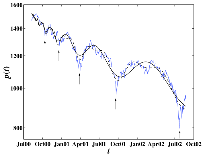
Figure 1: The price trajectory of the US S&P 500 index from August 21, 2000 to August 24, 2002. A clear decaying log-periodic structure is visible, implying a well developed anti-bubble. The upward arrows indicate the very large and sharp drops or crashes in the price evolution, which will be modelled in this paper as approximate local singularities. The lines are the fits by the log-periodic power law formula (1) including a single angular log-frequency $\omega$ (continuous line) as well as its harmonics $2\omega$ (dashed line).

Figure 1 shows the USA S&P 500 index from August 21, 2000 to August 24, 2002 and the fits by the log-periodic power law formula

$$\ln[p\left(t\right)]\approx A+B(t-t_{c})^{\alpha}+C(t-t_{c})^{\alpha}\cos\left[\omega\ln\left(t-t_{c}\right)-\phi\right]~{},$$ (1)

(where $t_{c}$ is the starting time of the anti-bubble) including a single angular log-frequency $\omega$ (continuous line) as well as its harmonics $2\omega$ (dashed line). These two theoretical curves constituted the main results of our previous work [23] which led us to issue a prediction for the future evolution of the US market (see also our web site for monthly updates of our predictions). Notwithstanding the remarkable capture of the overall decay and of the expanding alternation of ups and downs, the five crashes outlines by the arrows are not accounted by this theory. These five crashes constitute an important characteristic of this time series which is much rougher and singular than predicted by the gentle cosine function used in expression (1). The importance of these five crashes can be seen both at the level of the geometrical description of the price time series and with respect to their meaning and implications in the overall organization of the social network of investors.

Our purpose is to propose a simple extension of expression (1) based on a renormalization group analysis of the critical behavior embodied by (1) that accounts very accurately for the presence of these five crashes. The theory developed here shows that expression (1) is nothing but the first Fourier component of a more complete infinite Fourier series expansion of the general critical log-periodic power law behavior. This extension rationalizes the hierarchical geometric series of the time occurrences of these five crashes. Within our new theory, the qualitative explanation for the occurrence of these five crashes is similar to that underlying crashes following speculative bubbles. The main qualitative ingredient of the theory is the existence of positive feedbacks, of the kind which has been documented to occur in stock markets as well as in the economy. Positive feedbacks, i.e., self-reinforcement, refer to the fact that, conditioned on the observation that the market has recently moved up (respectively down), this makes it more probable to keep it moving up (respectively down), so that a large cumulative move may ensue. In a dynamical model, positive feedbacks with nonlinear amplifications have been shown to give rise to finite-time singularities which are good mathematical representations of the market price trajectory on the approach to crashes [20, 7]. However, such dynamical formulation describes only the price trajectory up to its singularity. It does not describe the rebound and ensuing evolution after the singularity. In this sense, our present approach is more powerful because it shows a deep connection between the existence and organization of the five crashes on the one hand and the overall log-periodic power law decay of the market crash on the other hand.

In an anti-bubble such as the regime of the S&P500 since August 2000, after a bottom, the positive feedbacks described above lead to the following qualitative scenario. First, the price rebounds as investors expect that the bad times may be behind them. However, the euphoria is short-lived as the fundamentals and the overall market sentiment are negative, leading to a slowdown and even reversal of the positive into a negative trend. The negative trend is then amplified by the collective herding behavior of investors, who, similarly to lemmings rushing over a cliff, run to sell, leading to each of these five observed crashes. Within our framework, these five crashes pertaining to the S&P500 anti-bubble phase are thus intrinsically endogenous to the market dynamics, similarly to most of the crashes found in many markets worldwide [14].

This paper is organized as follows. In Sec. 2, we summarize the main concepts and results of a renormalization group theory of the anti-bubble regime, leading to solutions taken the form of Weierstrass-type functions [5]. We present our fitting procedure in Sec. 3.1 and the determination of the relevant number of terms in our model in Sec. 3.2. The class of models describing the discretely scale invariant hierarchy of crashes is presented in Sec. 3.3. Its variants leading to non-singular price trajectories are investigated in Sec. 3.4. In Sec. 4, we then use three variants with different choices of the phases of the log-periodic components to offer a new analysis of the prediction of the S&P 500 index in the coming year. This set of predictions extend and refine our previous prediction [23]. Sec. 5 concludes.

2 Construction of Weierstrass-type functions

$\ln[p\left(t\right)]$ given by expression (1) is endowed with the symmetry of discrete scale invariance [18]. Indeed, multiplying $t-t_{c}$ by the factor $1/\gamma=e^{2\pi/\omega}$, we have

$$\ln[p\left((t-t_{c})/\gamma\right)]=A{\mu-1\over\mu}~{}+~{}{1\over\mu}\ln[p\left(t-t_{c}\right)]~{},~{}~{}{\rm with}~{}~{}\mu=\gamma^{\alpha}~{}.$$ (2)

Equation (2) expresses the fact that the prices, at two times related by a simple contraction with factor $\gamma$ of the interval since the beginning of the anti-bubble, are related themselves by a simple contraction with factor $\mu$ (up to the additive term $A(\mu-1)/\mu$). The scale invariance equation (2) is a special case of a general one-parameter renormalization group equation, which captures the collective behavior of investors in speculative regimes (see [19] for a pedagogical introduction to the ideas of the renormalization group as applied to finance). Using the renormalization group (RG) formalism on the stock market index $p$ amounts to assuming that the index at a given time $t$ is related to that at another time $t^{\prime}$ by the general transformations (4) and (5) below, first proposed for the stock market in Ref. [22] on the variable

$${\mathcal{F}}(x)=\ln[p(t)]-\ln[p(t_{c})]~{},$$ (3)

such that $F=0$ at the critical point at $t_{c}$. The first expression on the distance $x=|t-t_{c}|$ to the critical point occurring at $t_{c}$ reads

$$x^{\prime}=R(x)~{},$$ (4)

where $R$ is called the RG flow map. The second expression describes the corresponding transformation of the price and reads

$${\mathcal{F}}(x)={\mathcal{G}}(x)+\frac{1}{\mu}{\mathcal{F}}[R(x)]~{}.$$ (5)

The constant $\mu>1$ describes the scaling of the index evolution upon a rescaling of time (4). The function ${\mathcal{G}}(x)$ represents the non-singular part of the function ${\mathcal{F}}(x)$ which describes the degrees of freedom left-over by the decimation procedure involved in the change of scale of the description. We assume as usual [6] that the function ${\mathcal{F}}(x)$ is continuous and that $R(x)$ is differentiable.

These equations (5) with (4) can be solved recursively to give

$${\mathcal{F}}=\sum_{n=0}^{\infty}\frac{1}{\mu^{n}}{\mathcal{G}}\left[R^{(n)}(x)\right]~{},$$ (6)

where $R^{(n)}$ is the $n$th iterate of the map $R$. To make further progress, one expands $R(x)$ as a Taylor series in powers of $x$. For our purpose, it is sufficient to keep only the first-order linear approximation

$$R(x)=\gamma x$$ (7)

of the map $R$ around the fixed point $R(x_{c})=x_{c}=0$. For the effect of the next order term proportional to $x^{2}$, see [3]. Equation (6) then becomes

$${\mathcal{F}}=\sum_{n=0}^{\infty}\frac{1}{\mu^{n}}{\mathcal{G}}\left[\gamma^{n}(x)\right]~{}.$$ (8)

For the special choice ${\mathcal{G}}(x)=\cos(x)$, expression (8) recovers the Weierstrass function, famous for the fact that it was proposed by Weierstrass in 1876 as the first example of a continuous function which is no-where differentiable. This opened up the field of “fractals” [4].

Following Ref. [5], the infinite series in (8) can be expressed in a more convenient way by (1) applying the Mellin transform to (8), (2) re-expanding by ordering with respect to the poles of the Mellin transform of ${\mathcal{F}}$ in the complex plane, and (3) perform the inverse Mellin transform to obtain an expansion for ${\mathcal{F}}$ in terms of power laws expressing the critical behavior of the solution of the RG equation (5). This set of operation amounts to a resummuation of the infinite series in (8) which is better suited to describe the critical behavior and its leading corrections to scaling. The result is that ${\mathcal{F}}(x)$ can be expressed as the sum of a singular part ${\mathcal{F}}_{s}(x)$ and of a regular part ${\mathcal{F}}_{r}(x)$ [5]:

$${\mathcal{F}}(x)={\mathcal{F}}_{s}(x)+{\mathcal{F}}_{r}(x)~{},$$ (9)

where

$${{\mathcal{F}}}_{s}(x)=\sum_{n=0}^{\infty}A_{n}x^{-s_{n}}~{},$$ (10)

with

$$A_{n}=\frac{\hat{{\mathcal{G}}}(s_{n})}{\ln\gamma}~{},$$ (11)

and

$$s_{n}=-m+i\frac{2\pi}{\ln\gamma}n~{},~{}~{}{\rm with}~{}~{}m={\ln\mu\over\ln\gamma}~{}.$$ (12)

The coefficients $A_{n}$ control the relative weights of the log-periodic corrections (resulting from the imaginary parts of the complex exponents $s_{n}$) to the leading power law behavior described by the first term $n=0$. The regular part ${\mathcal{F}}_{r}(x)$ does not exhibit any singularity at $x=0$ or anywhere else and will not be considered further.

As an illustration, for the Weierstrass case with ${\mathcal{G}}(x)=\cos(x)$, for large $n$, the coefficients $A_{n}$ are given by

$$A_{n}=\frac{1}{\ln\gamma}\frac{1}{n^{m+0.5}}{\rm{e}}^{i\psi_{n}}~{},{\rm with}~{}~{}\psi_{n}=\omega n\ln(\omega n)~{}~{}{\rm and}~{}~{}\omega={2\pi\over\ln\gamma}~{}.$$ (13)

More generally, Ref. [5] has shown that, for a large class of systems, the coefficients $A_{n}$ of the power expansion of the singular part ${\mathcal{F}}_{s}(x)$ can be expressed as the product of an exponential decay by a power prefactor and a phase

$$A_{n}={1\over\ln\gamma}~{}~{}{1\over n^{p}}~{}e^{-\kappa n}~{}e^{i\psi_{n}},~{}~{}~{}~{}{\rm for~{}large}~{}~{}n~{},$$ (14)

where $p$, $\kappa\geq 0$ and $\psi_{n}$ are determined by the form of ${\mathcal{G}}(x)$ and the values of $\mu$ and $\gamma$. Systems, with quasi-periodic ${\mathcal{G}}(x)$ and/or such that ${\mathcal{G}}(x)$ has compact support, have coefficients $A_{n}$ decaying as a power law $A_{n}\sim n^{-p}$ ($\kappa=0$) leading to strong log-periodic oscillatory amplitudes. If in addition, the phases of $A_{n}$ are ergodic and mixing, the observable presents singular properties everywhere, similar to those of “Weierstrass-type” functions (13).

In the following, we restrict our attention to the “Weierstrass-type” class of models with $\kappa=0$ and extend the log-periodic power law formula (2) for the fit of empirical price time series by using the class of models ${{\mathcal{F}}}_{s}(x)$ given by (10) with the parametrization (14) with $\kappa=0$. Specifically, we shall use the following function for the fit of price time series:

$${{\mathcal{F}}}(x)=A+Bx^{m}+C\sum_{n=1}^{N}n^{-m-0.5}{\rm{e}}^{i\psi_{n}}x^{-s_{n}}~{},$$ (15)

where $A,B$ and $C$ are three parameters and $N$ is the number of log-periodic harmonics kept in the description. In the second term of the right-hand-side of (15), we have used $s_{n=0}=-m$ as seen from (12). We shall play with different parameterizations for the phases $\psi_{n}$, which can have forms different from $\psi_{n}=\omega n\ln(\omega n)$ given in (13) for the Weierstrass function. We shall also test the robustness of the fits with (15) by using the more general function

$$\ln[p(t)]=A+Bx^{m}+{\Re{\left(\sum_{n=1}^{N}C_{n}{\rm{e}}^{i\psi_{n}}x^{-s_{n}}\right)}}~{},$$ (16)

where ${\Re{()}}$ stands for the real part. Eq. (15) is recovered for $C_{n}=C/n^{m+0.5}$.

3 Description of the S&P500 anti-bubble by multiple singularities

3.1 Fitting procedure

The USA S&P 500 daily price series of the 2000 anti-bubble from August 21, 2000 to August 24, 2002, as shown in Fig. 1, is fitted with expression (16) by using a standard mean-square minimization procedure. We exploit the linear dependence of $\ln[p(t)]$ on the parameters $A,B$ and $C_{n}$ as follows. Rewriting formula (16) as

$$y(x)=A+Bf(x;\Phi)+\sum_{n=1}^{N}C_{n}g_{n}(x;\Phi)~{},$$ (17)

where $\Phi$ encapsulates all the non-linear parameters, given the data set $\{(x_{j},y_{j}):j=1,...,J\}$, the function to minimize is

$$Q(A,B,C_{n};\Phi)=\sum_{j=1}^{J}[y_{j}-y(x_{j})]^{2}~{}.$$ (18)

Following [15, 8], the $N+2$ linear parameters $A$, $B$ and $C_{n}$ are slaved to the nonlinear parameters $\Phi$ by solving the following linear equations:

$$\partial Q(A,B,C_{n};\Phi)/\partial(A,B,C_{n})=0~{}.$$ (19)

Let $\vec{A}=[\vec{I},\vec{f},\vec{g}_{1},\cdots,\vec{g}_{N}]$, where $\vec{I}$ is the identity column vector of $J$ elements, $\vec{f}=[f(x_{1}),f(x_{2}),\cdots,f(x_{J})]^{T}$ and $\vec{g}_{n}=[g_{n}(x_{1}),g_{n}(x_{2}),\cdots,g_{n}(x_{J})]^{T}$. Then the solution of Eq. (19) is

$$[A,B,C_{1},\cdots,C_{N}]^{T}=(\vec{A}^{T}\vec{A})^{-1}(\vec{A}\vec{y})^{T}~{},$$ (20)

where $\vec{y}=[y_{1},y_{2},\cdots,y_{J}]^{T}$. In the minimization of $Q(A,B,C_{n};\Phi)$ given by (18), the linear parameters $A$, $B$ and $C_{n}$ are determined accordingly to Eq. (20) as a function of the nonlinear parameters $\Phi$. The minimization process then reduces to minimizing $Q(A,B,C_{n};\Phi)$ with respect only to the nonlinear parameters $\Phi$. In order to obtain the global solution, we employ the taboo search [2] to determine an “elite list” of solutions as the initial solutions of the ensuing line search procedure in conjunction with a quasi-Newton method. The best fit is regarded to be globally optimized.

3.2 Jack-knife method to truncate the infinite series

For a practical implementation, it is necessary to truncate the infinite series in (16) and (17) at a finite order $N$. The larger $N$ is, the finer are the structures, as seen from the fact that, using (12), the real part of $x^{-s_{n}}$ equal to $x^{m}\cos\left[\omega n\ln(t-t_{c})\right]$ involves faster and faster oscillations as $n$ increases. Using a larger number $N$ of terms in (16) and (17) is bound to improve the quality of the fit by construction since the mean-square minimization with $N+1$ terms is obviously encompassing the mean-square minimization with $N$ terms, this later case being retrieved by imposing $C_{N+1}=0$. We thus need a criterion for characterizing the trade-off between the improvement of the fits on one hand when increasing $N$ and the associated increase in complexity (or lost of parsimony). For this, we adapt the Jack-knife method [24] in the following way. For a fixed $N$, we take away one observation $(x_{k},y_{k})$ from the time series $\{(x_{j},y_{j}):j=1,\cdots,J\}$, estimate the best fit characterized by its nonlinear parameters $\Phi_{k}$ using all observations but $(x_{k},y_{k})$, and try to predict $\hat{y}_{k}$, using the estimated function. We then repeat this procedure for every observation and get the average “prediction error”

$$\sigma_{N}=\left[\frac{1}{J}\sum_{j=1}^{J}(y_{j}-\hat{y}_{j})^{2}\right]^{1/2}~{},$$ (21)

which is a function of $N$. The optimal $N$, noted $N^{*}$, is such that by

$$\sigma_{N^{*}}=\min_{N}\{\sigma_{N}:N\in{\mathcal{N}}\}~{}.$$ (22)

This Jack-knife method is used usually for a sample of large size, generated by an unknown but fixed regression curve (e.g. a polynomial of an unknown degree). By the Jack-knife method, one determines once and for all the preferable degree of the approximating polynomial for the whole sample, i.e., the regression curves do not change from one sample point to another sample point. If the size of the time series $J$ is too large, $\sigma_{N}$ tends asymptotically to the the r.m.s. $\chi_{N}$ of the fit errors in the jack-knife test which tends to the r.m.s. $\chi$ of the fit errors with no points deleted. Hence, $\sigma_{N}$ is a monotonously decreasing function of $N$. Since we are interested in predictions over more than a one day horizon to minimize the impact of market noise, we extend the Jack-knife by partitioning the time series into groups of $u$ successive points. In each fit, a group of points are deleted and the previous Jack-knife method is applied simultaneously to the $u$ consecutive points to determine which $N$ leads to their best and most robust prediction.

We fit the S&P500 time series by Eq. (16) for $N=1,\cdots,10$. This process is repeated for $u=1,\cdots,5$. The set of free nonlinear parameters is $\Phi_{N}=(t_{c},m,\omega,\psi_{1},\cdots,\psi_{N})$. In all these fits, we find a very robust value for the fitted critical time (which is the theoretical starting time of the 2000 anti-bubble) given by $t_{c}={\rm{August~{}8,~{}2000}}\pm 10$ days. This result is in good agreement our previous result $t_{c}={\rm{August~{}9\pm 5,~{}2000}}$ obtained by varying the beginning of the fitted time window [23].

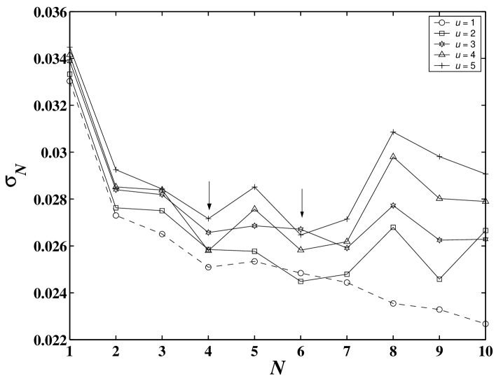
Figure 2: Standard deviation $\sigma_{N}$ of the errors in predicting the values of $u$ successive data points as a function of the number $N$ of terms in the series (15) defining the model used to fit the data. This constitutes a slight generalization of the Jack-knife method. The downward pointing arrows indicate the first two minima of $\sigma_{N}$ at $N=4$ and $N=6$ for $u>1$. The “global” minimum lies at $N=6$.

Figure 2 illustrates how we determine the optimal value for the number $N$ of terms in (16) using the extended Jack-knife method describe above. The dashed line with open circles corresponds to deleting only one point ($u=1$). In contrast with the monotonous decrease of $\sigma_{N}$ obtained for $u=1$, two local minima at $N=4$ and $N=6$ occur for all $u>1$, while the best minimum of $\sigma_{N^{*}}$ defined by (22) is obtained for $N=6$. We shall thus perform all our fits with six terms in the series (16) and (17).

3.3 A parsimonious model of the discrete hierarchy of five crashes

Within the present RG theory whose solution is expressed in the form of the “Weierstrass-type functions” (8), additional singularities other than that occurring by definition at $x_{c}=0$ appear when the phases $\psi_{n}$ in (14) all vanish so that all log-periodic power laws $x^{-s_{n}}$ in the expansion (10) are perfectly in phase for $x$ coincident with the infinitely discrete sets $x_{q}=1/\gamma^{q}$ with $q$ integer. Appendix B of Ref. [5] demonstrates using a renormalization group method applied to the series (10) that ${\mathcal{F}}_{S}(x)$ behaves, in the vicinity of these singular points $x_{q}$, as

$${\mathcal{F}}_{S}(x)\sim{\rm constant}+c|x-x_{q}|^{m-{1\over 2}}~{},$$ (23)

where $c$ is a constant. Thus, for $0<m<1/2$, spikes develop that correspond to a divergence of ${\mathcal{F}}_{S}(x)$ as $x\to x_{q}=1/\gamma^{q}$. For $1/2<m<3/2$, ${\mathcal{F}}_{S}(x)$ goes to a finite value as $x\to x_{q}$ but with an infinite slope (since $0<m-{1\over 2}<1$). The appearance of this set of singularities described by (23) is fundamentally based on the coherent “interferences” between all log-periodic oscillations in the infinite series expansion (10). These singularities disappear as soon as the phases are a function of $n$ due to the ensuing dephasing. In particular, for generic phase functions, the phases are ergodic as a function of $n$ and the singularities give place to no-where differentiable function (for $m<1$) [5].

Therefore, in order to reconstruct the five crashes shown in Figure 1, we first impose $\psi_{n}=0$ and search for the best fit of the S&P500 time series by expression (15) with $C_{n}=C/n^{m+0.5}$, $n=1,...,N$, truncated at $N=6$. Compared with the more general expression (16), equation (15) has only three linear parameters $A$, $B$ and $C$ instead of eight ($A$, $B$, $C_{1}$, $\cdots$, and $C_{6}$). We fit the S&P500 data from August 21, 2000 to August 24, 2002 and exclude the later data (the last four months at the time of writing) because August 24, 2002 is close to the end of the last complete log-periodic oscillations and the later data contains only a small part of the next extrapoled cycle. Our tests show that taking into account such a fraction of a log-periodic cycle in such an expanding anti-bubble may have a significant impact in the quality of the fits. Similarly, when we fit the time series ending in March 2002 at which the preceding cycle has completed less than its period, the retrieved log-periodic structure is quite distorted. We shall come back to this issue in details in Sec. 4 regarding its impact on the prediction of the future.

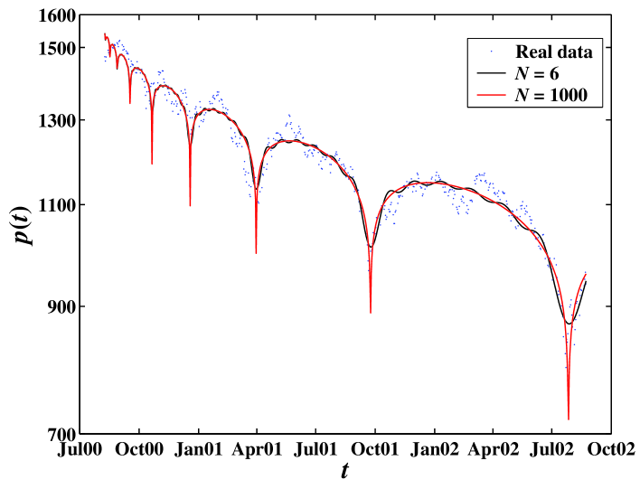
Figure 3: Fit of the price trajectory of the US S&P 500 (dots) by the model defined by Eq. (15) with $N=6$ and $\psi_{n}=0$. The fitted function is shown as the continuous wiggly line. The values of the fitted parameters are: $t_{c}={\rm{July~{}26,2000}}$, $m=0.53$, $\omega=11.43$, $A=7.39$, $B=-0.0141$, and $C=-0.0022$. The r.m.s. of the fit residuals is $0.0256$. The smooth continuous curve exhibiting local singularities (sharp drops) is constructed by inserting these fitted parameters into Eq. (15) with $N=1000$.

Figure 3 shows the best fit (in thick wiggly line) of the S&P500 index with formula (15) with $\psi_{n}=0$, $C_{n}=C/n^{m+0.5}$, $n=1,...,N$, truncated at $N=6$. The values of the parameters are $t_{c}={\rm{July~{}26,2000}}$, $m=0.53$, $\omega=11.43$, $A=7.39$, $B=-0.0141$, and $C=-0.0022$. The r.m.s. of the fit residuals is $0.0252$ (with only three free nonlinear parameters). In comparison, the r.m.s. of the fit residuals with expression (1) is $0.0325$ (four free nonlinear parameters) and with the extension including the second harmonic is $0.0265$ (five free nonlinear parameters). Since $C$ is determined from the fit with $N=6$, it can be used to extrapolate to the large $N$ limit and we thus also show the formula for $N=1000$ (thin smooth line with sharp troughs), which approximates very well the singularities at the five times of the crashes. Since $m=0.53$ is larger than $1/2$, the fit selects the class of singularities with finite end-log(price) and infinite slope. However, since $m$ is so close to the borderline value $0.5$, the price trajectory predicted by (23) is essentially undistinguishable numerically from a logarithmic singularity of the form ${\mathcal{F}}_{S}(x)\sim\ln|x-x_{q}|$. Such logarithmic singularities have been derived from a simple theory of positive feedback on risk aversion [1] and has been used as a trick to remove the exponent parameter from the fitting procedure [26, 25] (see however [11]).

This model reproduces remarkably well the structure of the S&P500 index, including both the overall log-periodic power law decay of the anti-bubble and the discrete hierarchy of the five crashes shown with arrows in Figure 1.

3.4 The role of the phase

Ref. [5] has shown that the dependence of the phases $\psi_{n}$ in Eq. (15) and Eq. (16) as a function of $n$ plays a central role in determining the structure of the solution. Expanding $\psi_{n}$ as $\psi_{n}=a_{p}n^{p}+...+a_{1}n+a_{0}$, where $p$ is the degree of the polynomial expansion of $\psi_{n}$ in powers of $n$, we find by fitting it to the price series for $p=0,1,2,3,4,5$ that only for $p=0$ and $p=1$ can one obtain the singular behavior obtained for $\psi_{n}=0$ (recovered for $p=0$) shown in figure 3. Intuitively, the reason is that only for $p=0$ and $p=1$ are the phases $\psi_{n}$ sufficiently regular to allow for constructive interference of the successive harmonics of Eq. (15) and Eq. (16).

Let us now sketch the proof of the following assertion: the necessary and sufficient condition for the existence of localized singularities is

$$\psi_{n}=a_{1}n+a_{0}~{}.$$ (24)

The crucial remark is that the cosine part $\cos[n\omega\ln(t-t_{c})-\psi_{n}]$ of the $n$th harmonic term in Eq. (15) can always be rewritten as $\cos[n\omega\ln(\tau)-a_{0}]$ with $\tau=(t-t_{c})/T$ where $T=\e^{a_{1}/\omega}$. The coefficient $a_{1}$ can thus be gauged away in a change of time units. Now, it is clear that for $\omega\ln(\tau)=2\pi k$ where $k$ is an integer, the cosines $\cos[n\omega\ln(\tau)-a_{0}]$ are equal to $\cos(a_{0})$ for all $n$. Thus, the infinite sum of the Weierstrass series is equal to $\cos(a_{0})$ times the sum obtained by putting all phases exactly equal to zero. This constitutes the sufficient part of the proof that phases of the form (24) are equivalent to phases identically equal to zero with respect to the occurrence of localized singularities (23). For the necessary part of the proof, it is easy to check by contradiction that a power $n^{p}$ with $p>1$ will give a moving amplitude for each harmonics thus breaking down the synchronization of the phases for the harmonics. One sees that the zero phase condition $\psi_{n}=0$ of the existence of localized singularities [5] is a special case of the linear phase condition (24).

For the fit with $p=1$, that is with expression (24), we find the following parameter values: $t_{c}={\rm{July~{}31,2000}}$, $m=0.54$, $\omega=11.35$, $a_{1}=49.56$, $a_{0}=3.35$, $A=7.37$, $B=-0.0125$, $C=0.0020$, with a r.m.s. of the fit residuals equal to $\chi=0.0249$. We find that the parameters $t_{c}$, $m$, $\omega$, $A$, $B$ and $C$ are very close to those obtained with the fit shown Fig. 3, indicating a good robustness with respect to the addition of the two parameters $a_{0}$ and $a_{1}$. Note also the very small improvement of the r.m.s. obtained by using (24) compared with the r.m.s. of $0.0252$ obtained by imposing $a_{0}=a_{1}=0$ and shown in Figure 3. As the addition of these two parameters $a_{0}$ and $a_{1}$ provides only a very minor improvement, it would not be qualified by using an Aikaike or information entropic criterion. In our investigation below on the potential of this formulation for prediction, we shall thus focus on the more parsimonious specification with zero phases $\psi_{n}=0$. Other tests not presented here confirm the over-determination of the Weierstrass-like formula with the two parameters $a_{0}$ and $a_{1}$ because it gives very poor prediction skills in comparison with the simpler model $\psi_{n}=0$.

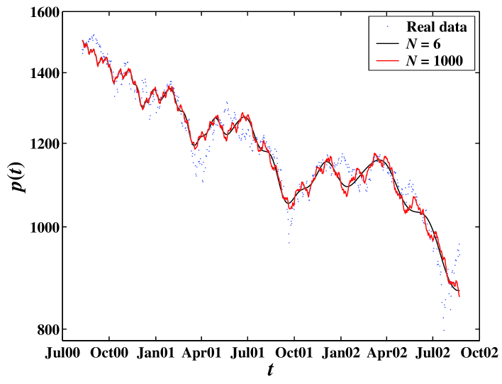
Figure 4: Fit of the price trajectory of the US S&P 500 (dots) using Eq. (15) with $N=6$ and $\psi_{n}=\omega n^{2}$. The values of the parameters are: $t_{c}={\rm{August~{}7,2000}}$, $m=0.69$, $\omega=10.61$, $A=7.32$, $B=-0.0043$, and $C=0.0008$. The r.m.s. of the fit residuals is $0.0312$. The thin wiggly curve is constructed by inserting the fitted parameters into Eq. (15) with $N=1000$. Freeing the parameter $\omega$ in the phase $\psi_{n}=\omega n^{2}$ by adopting $\psi_{n}=an^{2}$ improves the goodness-of-fit to the r.m.s. of fit residuals equal to $\chi=0.274$.

To demonstrate the phenomenon of destructive interferences between the log-periodic oscillations of successive harmonics, let us consider the simple model $\psi_{n}=\omega n^{2}$. Following the same fitting procedure as in Sec. 3.3 with $N=6$, Fig. 4 shows the best fit (smooth continuous line) compared with the data (dots), corresponding to the parameters $t_{c}={\rm{August~{}7,2000}}$, $m=0.69$, $\omega=10.61$, $A=7.32$, $B=-0.0043$, and $C=0.0008$. The r.m.s. of the fit residuals is $0.0312$ (three free nonlinear parameters). The wiggly continuous curve is constructed by inserting these fitted parameters into Eq. (15) with $N=1000$, leading to a continuous but non-differentiable function (in the limit $N\to+\infty$). Notice that these two functions capture quite well the complex structure of ups and downs occurring at multiple scales but fall short of fitting the five sharp drops of crashes analyzed in the previous Sec. 3.3. Freeing parameter $\omega$ and adding one parameter $a$ in the fitting procedure of the quadratic model $\psi_{n}=an^{2}$ improves the goodness-of-fit by decreasing r.m.s. of the fit residuals to $\chi=0.274$ with parameters moved to $t_{c}={\rm{August~{}3,2000}}$, $m=0.59$, $\omega=11.2$, $a=454$, $A=7.355$, $B=-0.0090$, and $C=0.0016$. But again, no sharp drops are reconstructed due to the incoherent interferences between the oscillations at different scales.

As a second illustrative example, let us take the phases corresponding to the asymptotic dependence of the phases of the Weierstrass function given by (13), that is, $\psi_{n}=\omega n\ln(\omega n)$. With $N=6$, we follow the same procedure as in Sec. 3.3. Fig. 5 shows the fitted function (smooth continuous line) with parameters $t_{c}={\rm{Jul~{}27,2000}}$, $m=0.67$, $\omega=11.18$, $A=7.34$, $B=-0.0051$, and $C=0.0009$. The r.m.s. of the fit residuals is $0.0309$. The wiggly continuous curve is constructed by inserting these fitted parameters into Eq. (15) with $N=1000$, leading to a continuous but non-differentiable function (in the limit $N\to+\infty$). Again, this model does not capture the five crashes described in Sec. 3.3. Replacing $\omega$ by two free parameters to obtain $\psi_{n}=bn\ln(cn)$ improves the goodness-of-fit by decreasing the r.m.s. of the fit residuals to $\chi=0.280$, but without much differences in the other parameters and no improvement to describe the 5 crashes.

In sum, Fig. 4 and Fig. 5 put in contrast with Fig. 3 show that the five crashes can be described accurately together with the overall anti-bubble structure by a coherent interference of the log-periodic harmonics occurring for the model with $\psi_{n}=a_{1}n+a_{0}$ while any other model of phases that desynchronizes the harmonics destroys the singularities and leads to a larger r.m.s. of the fit residuals.

4 Predictions

Up to now, we have shown that the model (15) with $\psi_{n}=0$ provides the best parsimonious description of the anti-bubble regime of the USA S&P500 index, improving upon our previous model [23] by fitting remarkably well the five crashes indicated by the arrows in Fig. 1. Notwithstanding the justification of our approach by the general renormalization group model, we do not have a microscopic model allowing us to justify rigorously the model (15) with $\psi_{n}=0$ based upon the detailed understanding of how each individual investor behavior is renormalized into a collective dynamics of this type. As an alternative, we propose that a crucial test of the model (15) with $\psi_{n}=0$ lies in its predictive power. We thus analyze its retro-active predictive power and then present a prediction for the future, that refines and complement our prediction issued in [23].

4.1 Retroactive predictions

By retroactive predictions, we mimick a real-life situation in which, at any present time $t_{\rm{last}}$, we fit the past time series up to $t_{\rm{last}}$, issue a prediction on the evolution of the price over, say, the next month and then compare it with the realized price from $t_{\rm{last}}$ to one month after $t_{\rm{last}}$.

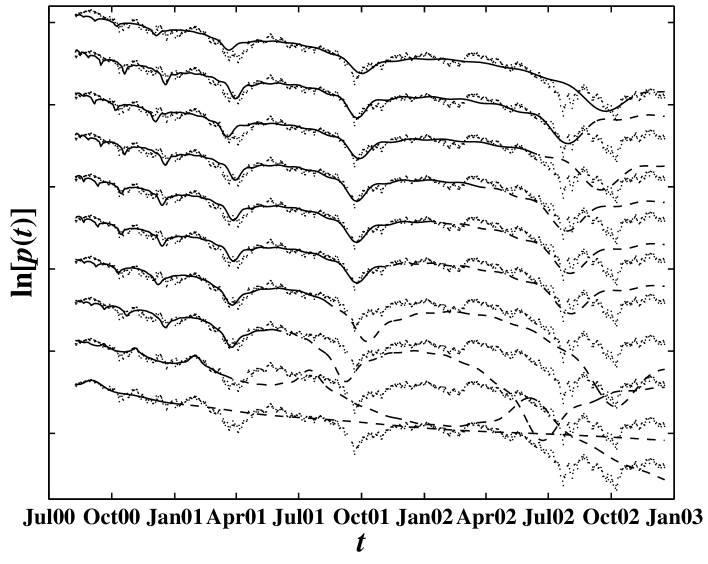
Figure 6: Ten predictions of the S&P 500 index using Eq. (15) with $N=6$ and $\psi_{n}=0$ for ten fictitious present dates: 02-Jan-2001, 15-Mar-2001, 25-May-2001, 07-Aug-2001, 23-Oct-2001, 04-Jan-2002, 19-Mar-2002, 30-May-2002, 12-Aug-2002, and 22-Oct-2002. Ten replicas of the price trajectory of the US S&P 500 (dots) have been generated and translated vertically to allow a simple comparison of the predictions. The continuous curves correspond to the fitted part of the mathematical function Eq. (15) with $N=6$ and $\psi_{n}=0$. The dashed parts give the extrapolations of these function beyond the fictitious present dates and thus correspond to the predictions.

Figure 6 compares the realized future prices to ten predictions of the S&P 500 index using Eq. (15) with $N=6$ and $\psi_{n}=0$ for ten fictitious present dates from Jan 02, 2001 (bottom) to Oct 22, 2002 (top). Showing ten translated replicas of the S&P 500 allows us to represent and compare the ten predictions in a synoptic manner. In each replica, the dots are the real price data, the smooth continuous line shows the fit up to the fictitious present $t_{\rm{last}}$ and the dashed line is the prediction beyond $t_{\rm{last}}$ obtained by extrapolating Eq. (15).

The first two predictions for $t_{\rm{last}}={\rm{Jan~{}2,2001}}$ and $t_{\rm{last}}={\rm{Mar~{}15,2001}}$ fail to give the correct trend. The predictions for $t_{\rm{last}}={\rm{May~{}25,2001}}$ and $t_{\rm{last}}={\rm{Aug~{}7,2001}}$ capture the trend of the price trajectory but are too pessimistic. However, these two predictions suggest that there is a significant endogenous drop in the beginning of September, 2001, before the 9/11 terrorist attack happened. In general, the predictions after $t_{\rm{last}}={\rm{Oct~{}23,2001}}$ are in excellent agreement with the real data and are very robust. In addition, the last three predictions are successful in suggesting the future happening of an instability in the form of two close sharp drops between July and November of 2002.

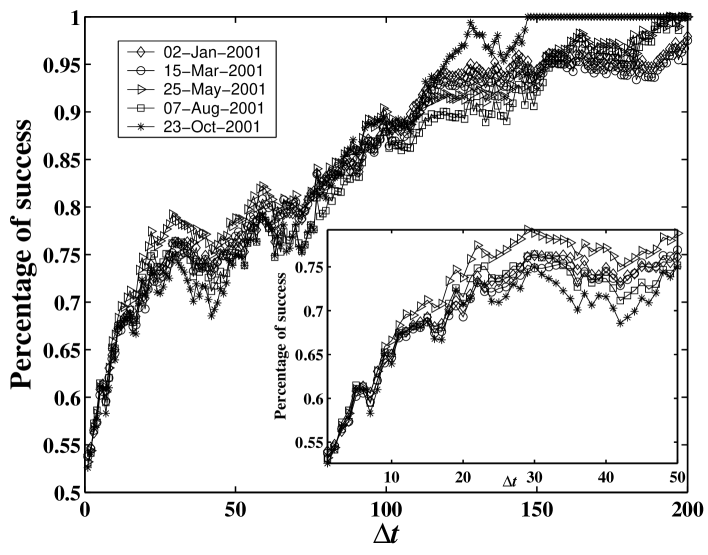
Figure 7: Percentage of success for the prediction of the signs of the returns over a time horizon of $\Delta t$ as a function of $\Delta t$ for five different starting dates of the strategies given in the upper-left inset. The lower-right inset gives a magnification for $\Delta t\leq 50$. See text for explanations.

Let us now quantify the predictive skill of Eq. (15) with $N=6$ and $\psi_{n}=0$ by calculating the percentage of success for the prediction of the sign of the return $r(t;\Delta t)=\ln[p(t+\Delta t)]-\ln[p(t)]$ from the fictitious present $t_{\rm{last}}$ to the time $t_{\rm{last}}+\Delta t$, that is, over a time horizon of $\Delta t$ days. For each successive fictitious present $t_{\rm{last}}$, a new prediction is issued to predict the sign of $r(_{\rm{last}};\Delta t)$. We investigate prediction horizons $\Delta t$ spanning from $1$ day to $200$ days. For each $\Delta t$, we calculate the success rate from a starting time $t_{\rm{enter}}$ to November, 21, 2002 and consider five different starting time $t_{\rm{enter}}$ to test for the robustness of the results. The results are presented in Fig. 7. The prediction success percentage increases with $\Delta t$ from a minimum of $53\%$ for $\Delta t=1$ day to above $90-95\%$ for $\Delta t>120$ days. This extraordinary good success for the larger time horizons only reflects the overall downward trend of the S&P500 market over the studied time period and is thus not a qualifier of the model. More interesting is the observation that the success rate increases above $70\%$ for $\Delta t>20$ days. In addition, the results are robust with respect to the changes of the starting date $t_{\rm{enter}}$. We consider the plateaus at about $75\%$ success rate in the range $\Delta=20\sim 70$ days to reflect a genuine predictive power of the model.

If indeed the model has predictive power, we should be able to use it in order to generate a profitable investment strategy. This is done as follows. For simplicity, we assume that a trader can hold no more than one share (position $+1$) or short no more than one share (position $-1$). In addition, a trader is always invested in the market, so that her position is $\pm 1$ at any time. For a given $\Delta t$, at a given time $t_{\rm{last}}$, if the model predicts that, at time $t_{\rm{last}}+\Delta t$, the price will go up ($r(t_{\rm{last}};\Delta t)>0$), the trader buys 2 shares at the price $p(t_{\rm{last}})$ if she was holding $-1$ share or holds her existing share if she has already one. Analogously, if the prediction shows that the price will go down ($r(t_{\rm{last}};\Delta t)<0$), she sells 2 shares at the present time $t_{\rm{last}}$ at the price $p(t_{\rm{last}})$ if she was holding $1$ share or holds her existing $-1$ short position if she is shorting already. Each prediction and reassessment of her position is performed with a time step of $\Delta t$ days. We do not include transaction costs or losses from the motion of the price during a transaction. Their impact can easily be incorporated and they are found not to erase the significant arbitrage opportunity documented here.

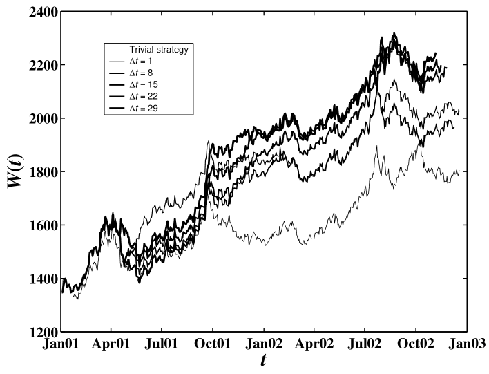
Figure 8: The running wealth $W(t)$ of a trader investing with a time step $\Delta t$ based on the prediction of the sign of the return over the time interval $\Delta t$. The origin of time is chosen as $t_{\rm{enter}}={\rm{Jan~{}2,2001}}$. Six time horizons are compared with the “short-and-hold” strategy (called trivial in the inset). See text for explanations.

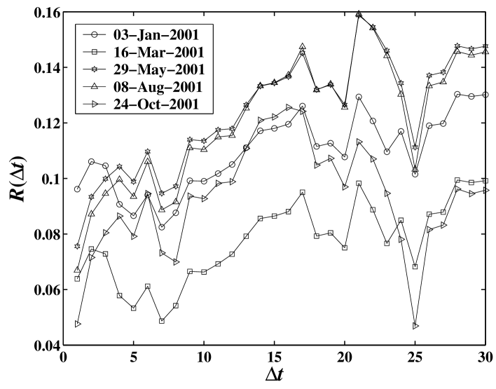
Figure 9: Daily Sharpe ratio $R(\Delta t)$ as a function of the time horizon $\Delta t$ for five different origin of time $t_{\rm{enter}}$.

The initial wealth of each trader is $+1$ share of stock at the initial time taken to be $t_{\rm{enter}}={\rm{Jan~{}2,2001}}$. Figure 8 shows the time dependence of the trader’s wealth $W(t)$ for different values of $\Delta t$. We compare this wealth with the “short-and-hold” strategy, the symmetric of the usual “buy-and-hold” strategy adapted to the overall bearish nature of the S&P500 price trajectory over the studied period. It is clear that all the strategies using our model outperform significantly the naive “short-and-hold” strategy. The corresponding Sharpe ratios, $R(\Delta t)$, defined as the ratio of the average daily return $\ln[W(t+1)]-\ln[W(t)]$ divided by the standard deviation of the daily return, are shown in Figure 9 as a function of $\Delta t$ for five different starting times $t_{\rm{enter}}$ of the strategies. Our trading strategies have a daily Sharpe ratio of the order of $0.1-1.4$. In comparison, the Sharpe ratio of the “short-and-hold” strategy is $0.06$. Thus, the impact of our strategy is roughly to double the Sharpe ratio. Translated into the standard yearly sharp ratio, a daily value $0.1-0.14$ gives a quite honorable value in the range $1.5-2.2$ compared with $0.9$ for the “short-and-hold.”

4.2 Forward predictions

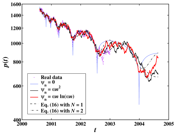
Figure 10: Forward predictions based on the analysis of the US S&P 500 index from August 21, 2000 to August 24, 2002 using Eq. (15) with $N=1000$ obtained with the three phase models $\psi_{n}$ indicated in the legend. The otherwise lines are predictions using (16) with $N=1$ (dashed line) and $N=2$ (dash-dotted line).

The predictions shown in Fig. 10 use the US S&P 500 index from August 21, 2000 to August 24, 2002 which is fitted by Eq. (15) with $N=6$ and three different phases $\psi_{n}=0$, $\psi_{n}=\omega n^{2}$ and $\psi_{n}=\omega n\ln(\omega n)$ respectively. Once the parameters of these three models have been determined, we construct the corresponding Weierstrass-type functions with $N=1000$ terms. The predictions are obtained as straightforward extrapolations of the three Weierstrass-type functions in the future. The predictions published in [23] using the log-periodic formula (1) with a single angular log-frequency $\omega$ (dashed line) and including its harmonics $2\omega$ (dash-dotted line) are also shown for comparison.

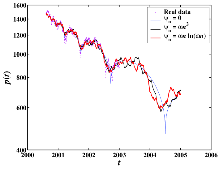
Figure 11: Same as Figure 10 based on the analysis of the US S&P 500 index from August 21, 2000 to January 8, 2003.

Fig. 11 is the same as Fig. 10 but is updated by including the US S&P 500 index data from August 21, 2000 to January 8, 2003. One can observe that the two predictions are very similar. The parameters of the corresponding fits are listed in Table 1.

According to these predictions, we can expect an overall continuation of the bearish phase, punctuated by some local rallies. An overall increasing market until the first quarter of 2003 is predicted, which should be followed by several months of more or less stable prices. Then, we predict a rather rapid descent (with maybe one or two severe ups and downs in the middle) which bottoms during the first semester of 2004. Quantitatively, the predictions suggests that the S&P 500 will culminate at about 1000 in the first quarter of 2003 and then dive down to 650 in early/mid 2004. These results are consistent with those in Ref. [23].

In spite of the robustness of the predictions, there is nevertheless a slight visible differences between Fig. 10 and Fig. 11. The latest predictions shown in Fig. 11 are shifted compared with those shown in Fig. 10 by a few months. Technically, we see that this comes from the existence of two dips in the second half of 2002, the first dip being fitted by the model in Fig. 10 while the second dip seems to have a stronger influence as shown in Fig. 11.

5 Discussion and Concluding remarks

We have proposed a straightforward extension of our previously proposed log-periodic power law model of the “anti-bubble” regime of the USA market since the summer of 2000 [23] and which is continuing to the present day. The generalization proposed here is using the renormalization group framework to model critical points. Using a previous work [5] on the classification of the class of Weierstrass-like function, we have shown that the five crashes that occurred since August 2000 can be accurately modelled by this approach, in a fully consistent way with no additional parameters. Our theory suggests an overall consistent organization of the investors forming a collective network which interact to form the pessimistic bearish “anti-bubble” regime with intermittent acceleration of the positive feedbacks of pessimistic sentiment leading to these crashes. We have complemented the descriptive analysis by developing and testing retrospective predictions, that confirm the existence of significant arbitrage opportunities for a trader using our model. We then conclude our analysis by offering a prediction for the unknown future. Obviously, only forward predictions constitute the ultimate proof of our claims. This exercise is an additional step in our constitution of a database of forward predictions whose statistical analysis will eventually allow us to confirm or disprove the validity of our models.

An additional feature may be pointed out: our analysis suggests that the five crashes are essentially of an endogenous origin, including the one in the first half of September 2001, often thought to have been provoked by the 911 terrorist attack. Our analysis suggests that the market was already on its way to a panic: the 911 event seems to have amplified the drop quantitatively without changing its qualitative nature. A similar conclusion was obtained for the crash of August-September 1998 often attributed to external political and economic events in Russia [10]. In this spirit, Ref. [14] has stressed that two-third of the major crashes in a large number of markets are of an endogenous origin and only the most dramatic piece of news (such as the announcement of World War I) are able to move the markets with an amplitude similar to the endogenous crashes.

Acknowledgments: We are grateful to V.F. Pisarenko for helpful discussions concerning the Jack-knife method and S. Gluzman for useful discussions on Weierstrass-type functions. This work was supported by the James S. Mc Donnell Foundation 21st century scientist award/studying complex system.

Table 1: Values of the parameters of the fits of the S&P500 index from Aug-09-2000 to $t_{\rm{last}}$ given in the first column with formula (15) for different models of the phases $\psi_{n}$. $\chi$ is the r.m.s. of the fit residuals.

$t_{\rm{last}}$	$\psi_{n}$	$t_{c}$	$m$	$\omega$	$A$	$B$	$C$	$\chi$
Aug-24-2002	0	19-Jul-2000	0.52	11.41	7.40	-0.0146	-0.0022	0.027
Aug-24-2002	$\omega n^{2}$	02-Aug-2000	0.69	10.59	7.33	-0.0044	0.0008	0.031
Aug-24-2002	$\omega n\ln(\omega n)$	27-Jul-2000	0.67	11.18	7.34	-0.0052	0.0010	0.030
Jan-08-2003	0	30-Jul-2000	0.82	10.37	7.31	-0.0019	-0.0004	0.036
Jan-08-2003	$\omega n^{2}$	31-Jul-2000	0.84	10.55	7.31	-0.0016	0.0003	0.035
Jan-08-2003	$\omega n\ln(\omega n)$	22-Jul-2000	0.83	11.07	7.31	-0.0017	0.0003	0.033

Figure 5: Fit of the price trajectory of the US S&P 500 (dots) using Eq. (15) with $N=6$ and $\psi_{n}=\omega n\ln(\omega n)$. The values of the parameters are: $t_{c}={\rm{July~{}27,2000}}$, $m=0.67$, $\omega=11.18$, $A=7.34$, $B=-0.0051$, and $C=0.0009$. The r.m.s. of the fit residuals is $0.0309$. The thin wiggly line is constructed by inserting the fitted parameters into Eq. (15) with $N=1000$. Freeing the parameter $\omega$ in the phase $\psi_{n}=\omega n\ln(\omega n)$ by adopting $\psi_{n}=bn\ln(cn)$ improves the goodness-of-fit to the r.m.s. of fit residuals equal to $\chi=0.280$.

References

- [1] J.-P. Bouchaud, R. Cont, A Langevin approach to stock market fluctuations and crashes, European Physics Journal B 6 (1998) 543-550.
- [2] D. Cvijovic, J. Klinowski, Taboo Search: An Approach to the Multiple Minima Problem, Science 267 (1995) 664-666.
- [3] B. Derrida, J. P. Eckmann, A. Erzan, Renormalization groups with periodic and aperiodic orbits, J. Phys. A 16 (1983) 893-906.
- [4] G.A. Edgar, ed., Classics on Fractals (Addison-Wesley Publishing Company, Reading, Massachusetts, 1993).
- [5] S. Gluzman, D. Sornette, Log-periodic route to fractal functions, Phys. Rev. E 65 (2002) 036142.
- [6] N. Goldenfeld, Lectures on phase transitions and the renormalization group (Addison-Wesley, Advanced Book Program, Reading, Mass., 1992).
- [7] K. Ide, D. Sornette, Oscillatory finite-time singularities in finance, population and rupture, Physica A 307 (2002) 63-106.
- [8] A. Johansen, O. Ledoit and D. Sornette, Crashes as critical points, International Journal of Theoretical and Applied Finance 3, 219-255 (2000).
- [9] A. Johansen, D. Sornette, Critical crashes, Risk 12 (1999) 91-94.
- [10] A. Johansen, D. Sornette, Financial “anti-bubbles”: Log-periodicity in Gold and Nikkei collapses, Int. J. Mod. Phys. C 10 (1999) 563-575.
- [11] A. Johansen, D. Sornette, Modeling the stock market prior to large crashes, Eur. Phys. J. B 9 (1999) 167-174.
- [12] A. Johansen, D. Sornette, Evaluation of the quantitative prediction of a trend reversal on the Japanese stock market in 1999, Int. J. Mod. Phys. C 11 (2000) 359-364.
- [13] A. Johansen, D. Sornette, Bubbles and anti-bubbles in Latin-American, Asian and Western stock markets: An emprical study, Int. J. Theoretical and Appl. Finance 4 (2000) 853-920.
- [14] A. Johansen and D. Sornette, Endogenous versus exogenous crashes in financial markets, preprint at cond-mat/0210509 (2002).
- [15] A. Johansen, D. Sornette, O. Ledoit, Predicting financial crashes using discrete scale invariance, Journal of Risk 1 (1999) 5-32.
- [16] B.B. Mandelbrot, The Fractal Geometry of Nature (New York, Freeman, 1983).
- [17] W. Press, S. Teukolsky, W. Vetterling, B. Flannery, Numerical Recipes in FORTRAN: The Art of Scientific Computing (Cambridge University, Cambridge, 1996).
- [18] D. Sornette, Discrete scale invariance and complex dimensions, Phys. Rep. 297 (1998) 239-270.
- [19] D. Sornette, Why Stock Markets Crash (Critical Events in Complex Financial Systems) (Princeton University Press, Princeton, NJ, 2003).
- [20] D. Sornette, K. Ide, Theory of self-similar oscillatory finite-time singularities in Finance, Population and Rupture, Int. J. Mod. Phys. C 14, (2003) 267-275.
- [21] D. Sornette, A. Johansen, Significance of log-periodic precursors to financial crashes, Quant. Finance 1 (2001) 452-471.
- [22] D. Sornette, A. Johansen, J.-P. Bouchaud, Stock market crashes, precursors and replicas, J. Phys. I France 6 (1996) 167-175.
- [23] D. Sornette, W.-X. Zhou, The US 2000-2002 market descent: How much longer and deeper? Quant. Finance 2 (2002) 468-481.
- [24] M. Stone, Cross-validatory choice and assessment of statistically prediction (with discussion), J. Roy. Statist. Soc. B 36 (1974) 111-147.
- [25] N. Vandewalle, M. Ausloos, P. Boveroux, A. Minguet, How the financial crash of October 1997 could have been predicted, Eur. Phys. J. B 4 (1998) 139-41.
- [26] N. Vandewalle, Ph. Boveroux, A. Minguet, M. Ausloos, The crash of October 1987 seen as a phase transition: amplitude and universality, Physica A 255 (1998) 201-210.
- [27] W.-X. Zhou, D. Sornette, Evidence of a worldwide stock market log-periodic anti-bubble since mid-2000, preprint at cond-mat/0212010.