Random walk through fractal environments

Abstract

We analyze random walk through fractal environments, embedded in 3–dimensional, permeable space. Particles travel freely and are scattered off into random directions when they hit the fractal. The statistical distribution of the flight increments (i.e. of the displacements between two consecutive hittings) is analytically derived from a common, practical definition of fractal dimension, and it turns out to approximate quite well a power-law in the case where the dimension $D_{F}$ of the fractal is less than 2, there is though always a finite rate of unaffected escape. Random walks through fractal sets with $D_{F}\leq 2$ can thus be considered as defective Levy walks. The distribution of jump increments for $D_{F}>2$ is decaying exponentially. The diffusive behavior of the random walk is analyzed in the frame of continuous time random walk, which we generalize to include the case of defective distributions of walk-increments. It is shown that the particles undergo anomalous, enhanced diffusion for $D_{F}<2$, the diffusion is dominated by the finite escape rate. Diffusion for $D_{F}>2$ is normal for large times, enhanced though for small and intermediate times. In particular, it follows that fractals generated by a particular class of self-organized criticality (SOC) models give rise to enhanced diffusion. The analytical results are illustrated by Monte-Carlo simulations.

I Introduction

We study the problem of particles performing a random walk through a fractal environment in 3-dimensional embedding space. The particles travel freely in the space not occupied by the fractal and are scattered off into random directions when they hit the fractal. We derive analytically the distribution $p_{r}$ of the random walk increments as a function of the dimension $D_{F}$ of the fractal set, and we calculate the diffusivity analytically, using the formalism of continuous time random walk (CTRW; e.g. Montroll1965 ), which we generalize here in order to include the case of defective (not normalized to one) distributions of walk-increments. The random walk is finally illustrated by Monte Carlo simulations.

The physical applications for the theory developed here are to systems consisting of a large number of spatially distributed, localized scatterers (accelerators), whose support forms a fractal set, suspended in a permeable medium, and in which particles move, with their dynamics being governed by collisions with the fractal: The particles move freely in the system except when they hit a part of the fractal (a scatterer), where they undergo the respective interaction, after which they leave the scattering center, possibly hit the fractal again, and so forth, performing thus a random walk in between subsequent interactions.

One application of the introduced theory is to particle transport in turbulent plasmas, whenever it can be asserted that the field inhomogeneities are distributed in a fractal way. This is implicitly claimed there where turbulent plasmas have successfully been modeled with self-organized criticality (SOC; about SOC see BTW ): In Ref. Isliker2001 , it has recently been shown that the unstable sites at temporal snap-shots during an avalanche in 3D form a fractal with dimension roughly $1.8$. This can be expected to hold for all SOC models whose evolution rules are of the type of Lu . Particles moving in the model will thus undergo the type of diffusion we analyze here.

Concrete examples of applications include the following: (i) Solar flares have been shown to be compatible with SOC (Lu ; Isliker ). The unstable sites of the SOC model, which represent small-scale current-dissipation regions (see Isliker ), cause the acceleration of particles, which perform thus a random walk of the type we analyze here. (ii) Though the question is still under debate, there are indications that the Earth’s magnetosphere exhibits structures compatible with SOC (e.g. magentosphere ). (iii) In inquiries on confined plasmas and the related transport phenomena, evidence has been collected that the confined plasma might be in the state of SOC (claimed in SOC , doubted though in Carbone ). Moreover, it is known that particles in confined plasmas undergo anomalous diffusion (confined ), a property which we will show also to hold often for the particles in the kind of systems we analyze here. (iv) A non-plasma, non-SOC example, where the theory developed here potentially can be applied, is the random walk of cosmic particles, which are scattered off the fractally distributed galaxies (e.g. Bak2001 ).

The investigation we present here is to be contrasted to two related, though characteristically different kinds of studies: — (I) In Ref. frac , random walks and diffusion along fractals are investigated, where the particles are forced to move along a fractal structure. The fractals investigated are connected fractals or percolation backbones. These studies are motivated by applications to the transport in porous media, or along percolation networks, and it is established that the diffusion in these systems is often anomalous. Differently to these studies, our random walkers cross the permeable space freely, they are not forced to follow the fractal structure, but they just occasionally hit the fractal. — (II) In Ref. (sand ), the random walk of sand grains in sand-pile (SOC) models is investigated, i.e. the direct transport of the unstable sites, which are found to undergo anomalous, enhanced diffusion. In contrast to these studies, when applying our theory to SOC models, we do not study the diffusion of the unstable sites (the transport of sand grains), but the diffusion of additional particles, foreign to the system (they are not contained in pure sand-pile models), which interact with the unstable sites, i.e. we freeze time in the avalanche model and let particles interact with the spatially distributed unstable sites. This is motivated through applications where the sand-pile does not model the evolution of real sand or rice-piles, but where it models ultimately the evolution of some kind of forces in dilute media (e.g. some kind of stress forces, or the magnetic or electric field in plasmas), in which the avalanche model merely gives the locations of the instabilities which affect particles moving otherwise freely in the system.

The fractal sets which constitute the environment we analyze are natural fractals, which exhibit self-similar scaling behavior only in a finite range, and which are made up of finite, 3-dimensional elementary volumes, small in size compared to the size of the fractal. According to Ref. Sinai1980 , such environments could be termed 3-dimensional, fractal Lorentz gas. Actually, any fractal set encountered in nature is a natural fractal in the sense introduced here, from the classical examples (the coast-line of Britain, cloud-surfaces, etc.; see Mandelbrot1982 ), to the localized scattering centers of the above mentioned applications mainly to plasma physics, which are yet small regions, with finite volumes, though.

In Sec. II, we will specify the notion of natural fractals, introduce the way we model the fractal scaling behaviour of natural fractals, derive analytically the probability distribution of the random walk increments for random walks through fractal environments, give the relations for the rate of unaffected escape from the system, and derive approximate forms of the distribution of jump increments. In Sec. III, the theory of Continuous Time Random Walk (CTRW) will be introduced and generalized to include the case of defective (not normalized to one) distributions of jump increments. The CTRW formalism will then be applied to determine analytically the diffusive behaviour for random walks through fractal environments, and to calculate the expected number of collisions with the fractal (in Sec. IV for fractal dimensions $D_{F}<2$, and in Sec. V for $D_{F}>2$). In Sec. VI, the analytical results will be compared to and illustrated by Monte-Carlo simulations. The results are summarized and discussed in Sec. VII, and Conclusions are drawn in Sec. VIII.

II Probability distribution of the increments of a random walk through a fractal environment

II.1 Specification of the problem; natural fractals

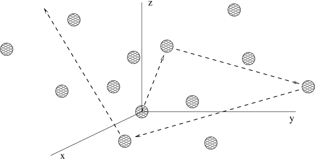
Figure 1: Sketch: The random walk in 3-dimensional space we analyze. A particle trajectory is indicated with an arrow. The small shaded regions are the elementary volumes $\delta V$ the fractal consists of (see Sec. II.1).

We assume a fractal $F$ embedded in 3-dimensional space ($\,{\rm I\kern-1.49994ptR}^{3}$) with a fractal dimension $D_{F}$ (e.g. box-counting or correlation dimension). We furthermore assume that there are particles (the random walkers) which travel freely in the empty (in the sense of not affecting the random walkers) space, but are scattered into random directions off the points belonging to the fractal $F$. Fig. 1 sketches the situation. Our interest in this Section is in the statistical distribution of the particles’ traveled distances in between two consecutive collisions with the fractal, i.e. of the random walk increments.

If we pose the problem in this form, then the fractals fall into two distinct classes: Imagine a particle to be situated at a point $\vec{x}_{i}$ belonging to $F$, somewhere in the interior. The particle actually ’sees’ the projection of the fractal onto a large imaginary sphere $S$ around $F$ and centered at $\vec{x}_{i}$, exactly as we do see the stars projected onto the celestial sphere. This sphere is 2-dimensional, so that, if $D_{F}<2$, the projection $F_{P}$ of $F$ onto $S$ has dimension $D_{P}=D_{F}<2$ (see e.g. Falconer1990 ). This implies that $F_{P}$ has zero measure (no volume). The possible trajectories for the particle are the straight lines originating from $\vec{x}_{i}$. The probability of such a trajectory to hit the fractal $F$ at all is the area occupied by $F_{P}$ on $S$, divided by the area of $S$; thus, the probability to hit the fractal is zero, the particle will almost never hit the fractal, it will almost surely escape from the system, and it does not make sense to determine a distribution of random walk increments.

On the other hand, if $D_{F}\geq 2$, then the projection of $F$ onto $S$ has dimension $D_{P}=2$, and the area occupied by $F_{P}$ on $S$ is positive (see e.g. Falconer1990 ). The probability of the particle to hit the fractal, which is again the area of $F_{P}$ on $S$, divided by the area of $S$, is finite, and it makes sense to determine a distribution of walk increments (for an isotropic fractal, we expect the probability to hit the fractal to be $1$, but there may be a finite probability for a particle to escape unaffected, without hitting the fractal at all, depending on the degree of spatial anisotropy of the concrete fractal under consideration).

This distinction holds for mathematical fractals, which per definition exhibit a scale-free scaling behavior (self-similarity or — possibly statistical — self-affinity) from their usually finite size down to all scales. Our interest here is though in what we term natural fractals: They are characterized by the following properties: (i) They are sampled only with a finite number of points. (ii) Their scaling behavior exhibits a lower cut-off, i.e. irrespective of the numerical method used to determine their fractal dimension, there will be a lower limit of scaling for the estimator. Correspondingly, there is a finite minimum separation distance $\delta$ between the points of the fractal. This property is partly a consequence of property (i). (iii) The elements the natural fractals consists of are not mathematical points, line-segments, or surface elements, but they represent finite, yet small 3-dimensional elementary volumes $\delta V$, at most of radial size $\delta/2$.

Properties (i) and (ii) characterize what one might call a finite fractal. They imply that $F=\{x_{i}\}_{i=1,...,n_{F}}$, i.e. $F$ is a finite collection of $n_{F}$ isolated points, with $\delta$ the smallest distance between them. If we assume the set $F$ to be contained in a sphere with radius $l$, then $F$ exhibits a fractal scaling behaviour for scales $r$ in the range $\delta\leq r\leq l$. The property (iii) makes the fractal natural in the sense that the points $x_{i}$ of $F$ represent actually small 3-dimensional volumes $\delta V$ of radial sizes smaller than $\delta/2$, with which a particle can interact through some forces, depending on the concrete physical application. We assume correspondingly an interaction cross-section $\rho^{2}\pi$ with cross-sectional radius $\rho$ to be associated with every point belonging to the fractal.

Since the $\delta V$ are 3-dimensional objects, we must require that that the volumes $\delta V$ should be smaller in radial size ($\rho$) than $\delta/2$, i.e. $\rho\leq\delta/2$: If $\rho$ were larger than $\delta/2$, then the fractal scaling of the natural fractal would break down already at the scale $2\rho$, the diameter of the elementary volumes $\delta V$, i.e. before reaching the scale $\delta$, which means that $\delta$ would have been inadequately determined and would have to be adjusted. Moreover, if the radius $\rho$ of the volumes $\delta V$ were in the range $\delta/2\leq\rho\leq\delta$, then near elementary volumes would over-lap, and they would be taken for one elementary volume.

In the frame of natural fractals, the random walk problem we pose takes a different shape: if the fractal were just finite, then all the particles would almost surely escape from the system without colliding with the fractal, since the probability to hit a finite set of isolated points with a straight line trajectory is obviously zero (the finite fractal in any case is a set of measure (volume) zero). Yet, since the fractals we analyze are natural, the isolated points of the fractal represent finite 3-dimensional volumes with a corresponding finte cross section, so that there is a finite probability for a particle to collide with these elementary volumes, and it makes sense to determine the corresponding distribution of walk increments.

A clarification is to be made concerning the scattering process: The scattering of the particles off the points of the fractal (the elementary volumes) is not scattering off hard spheres. We consider the elementary volumes as regions into which particles can penetrate, they will though be affected by some forces inside these regions. This is realistic since our main application is to plasma-physics, where the elementary volumes are typically regions where an electric field resides.

Last, we note that the radial size $l$ of the entire fractal is of course finite in any reasonable physical application. The derivations we will give in the following are consequently made for the case of finite fractals ($l<\infty$), it will though turn out that $l$ appears just as an arbitrary exterior parameter and therewith is allowed to take arbitrarily large values (Secs. II.3.1 and II.3.2). It will furthermore turn out that several characteristics of the problem we analyze assume finite asymptotic values if $l$ becomes very large (Secs. II.4 and II.5). We will thus include in our treatment the case of what we term asymptotically large systems, by which we mean systems where $l$ is so large that the asymptotic, large $l$ behaviour is practically reached, and we may let $l\to\infty$ in the respective relations. In Sec. II.4, the notion of ’asymptotically large’ fractals will be given a more precise meaning. Systems smaller than asymptotically large will be termed finite systems. Asymptotically large systems are of interest in applications above all to astrophysical plasma-systems, where fractals may indeed be very large.

II.2 The fractal scaling behaviour

Let us choose an arbitrary reference point $\vec{x}_{i}$ of the fractal, somewhere in the interior (to neglect boundary effects). Let $n_{i}(r)$ denote the number of points belonging to the fractal $F$ in the 3-dimensional sphere around $\vec{x}_{i}$ with radius $r$ ($r\leq l$, with $l$ the radial size of the fractal). Since $F$ is a fractal with dimension $D_{F}$, it is expected that

$$n_{i}(r)=A_{i}\,r^{D_{F}^{(i)}},$$ (1)

with $A_{i}$ a constant (Eq. (1) is based on the mass-scaling definition of fractal dimension, which is a common, practical definition of fractal dimension, see e.g. Mandelbrot1982 ). Eq. (1) holds actually in the limit $r\to 0$, but in practice it is known that the scaling behavior appears often already clearly at finite $r$, and the limit $r\to 0$ is not feasible. It is also worthwhile noting that Eq. (1) defines the local fractal dimension $D_{F}^{(i)}$, which may fluctuate with different reference points $\vec{x}_{i}$, the more, the less numerous the points of the fractal are. The average of Eq. (1) over the whole fractal $F$ is yet well defined (else $F$ would in practice not be called a fractal). In our applications, we are interested in statistical results, averaged over the entire fractal, i.e. over all possible reference points $\vec{x}_{i}$, so that in the following we use a single scaling behaviour

$$n(r)=Ar^{D_{F}}$$ (2)

everywhere, which corresponds to the average of the local $n_{i}(r)$ [Eq. (1)] over $i$. The constant $A$ is determined as follows: With every point $\vec{x}_{i}$ of the fractal is associated a scale $\delta_{i}$ — the distance to the nearest neighbour —, at which the local scaling behaviour $n_{i}(r)$ breaks down ($n_{i}(\delta_{i})=1$, so that $n_{i}(r)=(r/\delta_{i})^{D_{F}^{(i)}}$), which determines the constant $A_{i}$ in Eq. (1), $A_{i}=(1/\delta_{i})^{D_{F}^{(i)}}$. The scale $\delta$ introduced in Sec. II.1, where the scaling breaks totally down, is understood as the minimum of all the $\delta_{i}$, $\delta:=\min_{i}[\delta_{i}]$. For the average $n(r)$ of Eq. (2), we have to use an average scale $\delta_{\ast}$ at which the scaling breaks down on the average (i.e. $n(\delta_{\ast})=1$). In the examples of fractals we will introduce below, we find the distributions of the $\delta_{i}$ to be very asymmetric: they show a clear peak, but exhibit a tail which extends to large $\delta_{i}$. Fig. 2 shows a typical example of a histogram of the $\delta_{i}$ for the set $F_{3}$ which will be introduced below in Sec. VI.1.1. This particlular shape of the distribution of the $\delta_{i}$ has as a consequence that the arithmetic mean value of the $\delta_{i}$ is not representative of an average scale, it overestimates it. We therefore define $\delta_{\ast}$ as the most probable value of the distribution of the $\delta_{i}$, determining it by a histogram of the $\delta_{i}$. The fractal scaling behaviour thus takes the form

$$n(r)=\left({r\over\delta_{\ast}}\right)^{D_{F}},$$ (3)

with $\delta\leq r\leq l$.

Since the radial size of the the fractal is $l$, it follows that $n(l)$ is the total number of points $n_{F}$ of the fractal, or, with Eq. (3),

$$n_{F}=\left(l\over\delta_{\ast}\right)^{D_{F}}.$$ (4)

This relation is actually analogous to the case of non-fractal sets: If we sample for instance a 3–dimensional cube of side-length $l$ with a resolution $\delta_{\ast}$, then we would obviously find $(l/\delta_{\ast})^{3}$ points. Eq. (4) holds of course only for points in the interior of the fractal, towards the edge it is biased by edge effects.

Figure 2: Histogram of the nearest neighbour distances $\delta_{i}$, for the set $F_{3}$ ($D_{F}=1.8$, $l=50$, $\delta=0.5$, see Sec. VI.1.1 and Table 1).

II.3 Analytical derivation of the probability distribution $p_{r}$ of the random walk increments

From Eq. (3), it follows that the number of points $m(r)\Delta r$ of the fractal in a spherical shell around an interior point $\vec{x}_{i}$ with inner radius $r$ and radial thickness $\Delta r$ is $m(r)\Delta r={d\over dr}n(r)\cdot\Delta r$, or

$$m(r)\Delta r={D_{F}\over\delta_{\ast}}\,\left({r\over\delta_{\ast}}\right)^{D_{F}-1}\,\Delta r.$$ (5)

With every point of the natural fractal is associated a cross-section $\rho^{2}\pi$, within which an approaching particle gets into contact (interacts) with a point (elementary volume) of the fractal (see Sec. II.1). The entire shell has thus a total cross-section $s(r)\Delta r=m(r)\Delta r\cdot\rho^{2}\pi$, i.e.

$$s(r)\Delta r=\rho^{2}\pi\,\frac{D_{F}}{\delta_{\ast}}\,\left(\frac{r}{\delta_{\ast}}\right)^{D_{F}-1}\,\Delta r.$$ (6)

In order this to hold, the different points of the fractal should not overlap or cover each other with their cross sections. In the direction perpendicular to the radius $r$ this is guaranteed by the fact that $\rho\leq\delta/2$, half the smallest separation distance of the points of the fractal, with $\rho$ the cross-sectional radius. In the radial direction, it is also guaranteed, as long as we let $\Delta r\leq\delta/2$, so that also in radial direction we can be sure that no point is hidden by the cross-sectional surface of another point in front of it.

Assume now that a particle has started from $\vec{x}_{i}$ and has traveled freely a distance $r$ into a random direction. The probability $q_{r}\,\Delta r$ to hit the fractal in the spherical shell between $r$ and $r+\Delta r$ is the ratio of the total cross-section of the shell (the occupied area), divided by the area of the shell, $q_{r}\,\Delta r=s(r)\Delta r/4\pi r^{2}$, or, with some rearrangements,

$$q_{r}\,\Delta r=\frac{D_{F}\rho^{2}}{4\delta_{\ast}^{3}}\,\left(\frac{r}{\delta_{\ast}}\right)^{D_{F}-3}\,\Delta r.$$ (7)

Our scope is to derive the probability $p_{r}\Delta r$ for a particle to travel freely a distance $r$ and then to hit the fractal in the spherical shell between $r$ and $r+\Delta r$, starting from an arbitrary point of $F$. To derive this probability, we divide the interval $[\delta,r]$, which the particle travels freely, into a large number of small intervals of size $\delta r$: $[r_{1},r_{2}]$, $[r_{2},r_{3}]$, …, $[r_{n-1},r_{n}]$, with $r_{1}=\delta$, $r_{n}=r$, and $r_{i+1}-r_{i}=\delta r$ for all $i$ (the interval $[0,\delta]$ is free of points of $F$, and thus has not to be taken into account, since there are no points of the fractal closer than $\delta$). The probability not to hit the fractal in the intervals $[r_{i},r_{i+1}]$ is $1-q_{r_{i}}\delta r$, so that the probability not to hit the fractal in all the small intervals up to $r$, and to hit it finally in the interval $[r,r+\Delta r]$ is

$$p_{r}\Delta r = (1-q_{r_{1}}\delta r)\cdot(1-q_{r_{2}}\delta r)\cdot\,...\,$$ (8)

$$\times\,...\,\cdot(1-q_{r_{n-1}}\delta r)\cdot q_{r}\Delta r,$$

or

$$p_{r}\Delta r=\begin{cases}\prod_{i=1}^{n-1}(1-q_{r_{i}}\delta r)\cdot q_{r}\Delta r,&\ {\rm for}\ n\geq 2,\\ q_{r_{1}}\Delta r,&\ {\rm for}\ n=1.\\ \end{cases}$$ (9)

By defining

$$\pi_{r}:=\prod_{i=1}^{n-1}(1-q_{r_{i}}\delta r),$$ (10)

$p_{r}$ can be rewritten as

$$p_{r}\Delta r=\begin{cases}\pi_{r}\cdot q_{r}\Delta r,&\ {\rm for}\ n\geq 2,\\ q_{r_{1}}\Delta r,&\ {\rm for}\ n=1.\\ \end{cases}$$ (11)

We have to evaluate the product $\pi_{r}$ in the limit $n\to\infty$, where the small intervals get infinitesimal. First, we note that

$$\ln(\pi_{r}) = \ln\left(\prod_{i=1}^{n-1}(1-q_{r_{i}}\delta r)\right)$$ (12)

$$= \sum_{i=1}^{n-1}\ln\left(1-q_{r_{i}}\delta r\right).$$

$q_{r_{i}}$ is always positive and bounded by ${D_{F}\rho^{2}\over 4\delta_{\ast}^{3}}\,\left({\delta\over\delta_{\ast}}\right)^{D_{F}-3}$, since $\delta\leq r\leq l$, and since the exponent is negative ($D_{F}-3<0$). The term $q_{r_{i}}\delta r$ gets thus arbitrarily small for $n\to\infty$, since this implies that $\delta r\to 0$ ($\delta r$ is something like $(r-\delta)/n$, or, independent of $r$, $(l-\delta)/n$), and we may thus use the approximation $\ln(1+x)\approx x$, for $x<<1$. Eq. (12) thus becomes

$$\ln(\pi_{r})\approx\sum_{i=1}^{n-1}-q_{r_{i}}\delta r,$$ (13)

which for $\delta r\to 0$ may be considered as a standard expression for the Riemann integral of $-q_{r}$, with limits $\delta$ and $r$,

$$\ln(\pi_{r})=\int\limits_{\delta}^{r}-q_{r\prime}\,dr\prime,$$ (14)

where due to the limit the approximation has become exact.

II.3.1 The case $D_{F}\neq 2$

Inserting for $q_{r}$ from Eq. (7) into Eq. (14), and solving for $\pi_{r}$, one finds that in the case $D_{F}\neq 2$

$$\pi_{r}^{(D_{F}\neq 2)}=\exp\left[-{D_{F}\rho^{2}\over 4\delta_{\ast}^{D_{F}}}\,{\left(r^{D_{F}-2}-\delta^{D_{F}-2}\right)\over D_{F}-2}\right].$$ (15)

The probability $p_{r}\Delta r=\pi_{r}\,q_{r}\,\Delta r$ (Eq. 11) for a particle to start from a point of the fractal, to travel freely a distance $r$, and then to hit the fractal in a layer of depth $\Delta r$ is thus, by inserting Eqs. (7) and (15), and by rearranging,

$$p_{r}^{(D_{F}\neq 2)}\Delta r = \exp\left[D_{F}\,\rho^{2}{\left(\left(\frac{r}{\delta_{\ast}}\right)^{D_{F}-2}-\left(\frac{\delta}{\delta_{\ast}}\right)^{D_{F}-2}\right)\over 4(2-D_{F})\delta_{\ast}^{2}}\right]$$ (16)

$$\times\,{D_{F}\,\rho^{2}\over 4\delta_{\ast}^{3}}\left(\frac{r}{\delta_{\ast}}\right)^{D_{F}-3}\cdot\Delta r,$$

where $\delta\leq r\leq l$.

Notably, the radial size $l$ of the fractal does not appear in the relation for $p_{r}$: $l$ determines only the upper cut-off of $p_{r}$, it does not influence its shape. The size $l$ is thus an exterior parameter of the problem we study and can take any value between $\delta$ and infinity, without leading to any contradiction: as shown in App. A, the normalization of $p_{r}$ never exceeds 1, whatever the value of $l$ is.

II.3.2 The case $D_{F}=2$

In the case $D_{F}=2$ we find from Eq. (7) and Eq. (14)

$$\pi_{r}^{(D_{F}=2)}=\exp\left[-{D_{F}\rho^{2}\over 4\delta_{\ast}^{D_{F}}}\,\ln\frac{r}{\delta}\right].$$ (17)

Eqs. (11), (7), and (17) yield

$$p_{r}^{(D_{F}=2)}\Delta r = \exp\left[-{D_{F}\,\rho^{2}\over 4\delta_{\ast}^{D_{F}}}\,\ln\frac{r}{\delta}\right]$$ (18)

$$\times\,{D_{F}\,\rho^{2}\over 4\delta_{\ast}^{3}}\left(\frac{r}{\delta_{\ast}}\right)^{D_{F}-3}\cdot\Delta r,$$

which can be further rearranged to become

$$p_{r}^{(D_{F}=2)}\Delta r={D_{F}\,\rho^{2}\over 4\delta_{\ast}^{3}}\left(\frac{\delta_{\ast}}{\delta}\right)^{-\frac{D_{F}\,\rho^{2}}{4\delta_{\ast}^{2}}}\left(\frac{r}{\delta_{\ast}}\right)^{D_{F}-3-\frac{D_{F}\,\rho^{2}}{4\delta_{\ast}^{2}}}\cdot\Delta r,$$ (19)

and is thus a pure power-law. Again, as in the case $D_{F}\neq 2$ [Eq. (16)], the radial size $l$ of the fractal appears just as an upper limit for the allowed values of $r$.

II.4 The rate for unaffected escape

$\pi_{r}$ as defined in Eq. (10) is the probability not to hit the fractal at all in $[\delta,r]$ [see the explanation before Eq. (8)], so that $\pi_{r}|_{r=l}$ is obviously the probability $\nu_{esc}$ not to hit the fractal at all, but to move unaffected by the fractal to the edge of the system and to finally escape. From Eq. (15) we find that for $D_{F}\neq 2$, after slightly rearranging,

$$\nu_{esc}(D_{F}\neq 2)=$$

$$\exp\left[\frac{D_{F}\rho^{2}\left(\left(\frac{l}{\delta_{\ast}}\right)^{D_{F}-2}-\left(\frac{\delta}{\delta_{\ast}}\right)^{D_{F}-2}\right)}{4(2-D_{F})\delta_{\ast}^{2}}\right],$$ (20)

and in the case $D_{F}=2$, from Eq. (17),

$$\nu_{esc}(D_{F}=2)=\exp\left[-{D_{F}\rho^{2}\over 4\delta_{\ast}^{D_{F}}}\,\ln\left(\frac{l}{\delta}\right)\right].$$ (21)

Eqs. (20) and (21) imply that, depending mainly on the values of $D_{F}$, $l$, $\delta$, $\delta_{\ast}$, and $\rho$, there possibly is a finite rate for unaffected escape, i.e. a finite fraction of the particles does not ’see’ the fractal and moves through the system without collisions until it finally leaves. Actually, for finite systems ($l<\infty$), there is in any case a finite rate of unaffected escape, which is the larger, the smaller the system size ($l$), the cross-sectional radius $\rho$, and the fractal dimension $D_{F}$ are. For very large systems though, $\nu_{esc}$ settles to an asymptotic value, which corresponds to the lowest possible escape rate for given $\rho$ and $D_{F}$. As explained in Sec. II.1, we will in the following call systems asymptotically large (in contrast to finite systems), if they are so large that $\nu_{esc}$ has practically settled to its asymptotic value, and we will determine $\nu_{esc}$ in their case by letting $l\to\infty$.

For asymptotically large systems ($l\to\infty$), we have the following cases, depending on the value of $D_{F}$:

• In the case $D_{F}>2$, we find from Eq. (20)

  $$\nu_{esc}(D_{F}>2,l\to\infty)=0,$$ (22)

  so that all particles will collide with the asymptotically large fractal.

• In the case $D_{F}=2$, Eq. (21) yields

  $$\nu_{esc}(D_{F}=2,l\to\infty)=0,$$ (23)

  and again all particles collide with the asymptotically large fractal.

• For $D_{F}<2$, we have from Eq. (20)

  $$\nu_{esc}(D_{F}<2,l\to\infty)$$

  $$=\exp\left[-\frac{D_{F}\rho^{2}}{4(2-D_{F})\delta_{\ast}^{2}}\left(\frac{\delta}{\delta_{\ast}}\right)^{D_{F}-2}\right],$$ (24)

  which is strictly smaller than $1$ (note that the argument of the exponential function is in any case negative and finite), so that there is a finite fraction $\nu_{esc}$ of particles which move through the system without having any encounter along their path with the asymptotically large fractal, until they escape.

In Fig. 3, the rate of unaffected escape $\nu_{esc}$ is plotted against $D_{F}$ for $D_{F}<2$, assuming asymptotically large systems ($l\to\infty$): the escape rate is high, and only when $D_{F}$ approaches quite close $2$, the escape rate drops to low values.

Figure 3: The escape rate $\nu_{esc}$ vs. the fractal dimension $D_{F}$, for $0<D_{F}<2$ and assuming asymptotically large systems ($l\to\infty$; see Sec. II.4).

It is to note that the particles which escape unaffected do not leave the system instantaneously, they remain in the system and move on a straight line path with their individual finite velocity, without ever colliding again with the fractal, until they reach the edge of the system and leave. In other words, the paths the escaping particles follow never and nowhere intersect the fractal. In the case of asymptotically large fractals, the time elapsing until an escaping particle reaches the edge of the system may of course be considerable and much larger than the time for which the particles are tracked.

In Appendix A, Eqs. (20) and (21) will be derived in an alternative way, and it will be shown that the possibly finite rate of unaffected escape is related to the fact that $p_{r}$ is not necessarily normalized to one, it actually holds that

$$\nu_{esc}=1-\mu,$$ (25)

where

$$\mu:=\int\limits_{\delta}^{l}p_{r}\,dr$$ (26)

is the normalization of $p_{r}$. The cases of finite escape rate (for asymptotically large ($l\to\infty$) as well for finite system size) correspond thus to the cases where $\mu<1$, i.e. to the cases where $p_{r}$ is defective.

II.5 Approximate forms of $p_{r}$

To determine possible approximate or asymptotic forms of $p_{r}$, we consider the logarithmic derivative of $p_{r}$ [Eq. (16)] for $D_{F}\neq 2$,

$${d\ln p_{r}^{(D_{F}\neq 2)}\over d\ln r}=-{D_{F}\,\rho^{2}\over 4\delta_{\ast}^{2}}\left({r\over\delta_{\ast}}\right)^{D_{F}-2}+\left(D_{F}-3\right).$$ (27)

The term $D_{F}-3$ stems from the power-law factor, and the correcting term from the exponential factor in Eq. (16). For $D_{F}<2$, the logarithmic slope asymptotically reaches $D_{F}-3$ for large $r$, being slightly distorted for small $r$, at most by the amount $(D_{F}\,\rho^{2}/4\delta_{\ast}^{2})\cdot(\delta/\delta_{\ast})^{D_{F}-2}$ (for the smallest $r$, i.e. $r=\delta$). Hence, for $D_{F}<2$, $p_{r}$ can be considered as an approximate power-law with index $D_{F}-3$, whose exact form is found from Eq. (16) on replacing $r$ in the exponential by its maximum possible value $l$,

$$p_{r}^{(a;\ D_{F}<2)}\Delta r = \exp\left[\frac{D_{F}\rho^{2}\left(\left({l\over\delta_{\ast}}\right)^{D_{F}-2}-\left({\delta\over\delta_{\ast}}\right)^{D_{F}-2}\right)}{4(2-D_{F})\delta_{\ast}^{2}}\right]$$ (28)

$$\times\,{D_{F}\,\rho^{2}\over 4\delta_{\ast}^{3}}\left(r\over\delta_{\ast}\right)^{D_{F}-3}\cdot\Delta r.$$

It follows that for $D_{F}<2$ the second moments ($\int r^{2}p_{r}\,dr$) are infinite (the moments are dominated by the asymptotic, large $r$ regime), so that the random walks in the cases $D_{F}<2$ are approximate realizations of Levy-flights: for large $r$, the $p_{r}^{(a;\ D_{F}<2)}$ are of the same form as the Levy distributions, namely power-laws with index between $-3$ and $-1$ (see e.g. Hughes1995 ), and it is actually the large $r$ regime which causes the second moments to diverge and the random walk statistics not to obey the Central Limit Theorem. A characteristic difference to the Levy distributions is though that the distributions $p_{r}^{(a;\ D_{F}<2)}$ are in any case defective, associated with a finite escape rate (Sec. II.4).

For $D_{F}>2$, the logarithmic slope in Eq. (27) is dominated by the first term on the r.h.s., which increases in magnitude with increasing $r$, so that $p_{r}$ is decaying exponentially for large $r$, which implies that the second moments are finite, and the corresponding random walks are governed by the Central Limit Theorem.

The case $D_{F}=2$ is a pure power-law without any approximation (Eq. 19), the second moment is obviously infinite, and the random walk is an approximate realization of a Levy-flight, as are the cases $D_{F}<2$, defective though in the case of finite systems (see Sec. II.4).

III Continuous time random walk, generalized to the case of defective distributions: theory

In order to determine the diffusive behavior of particles analytically, we follow the formalism of Continuous Time Random Walk (CTRW; see Montroll1965 ) in the version of the velocity model (see Zumofen1993 ; Drysdale1998 ). In this approach, it is assumed that each spatial walk increment $\vec{r}$ is performed in finite time $\tau$, where $r(\equiv|\vec{r}|)$ and $\tau$ are related through the velocity $v$ of the walker, which we assume to be arbitrary and constant. If we would not take into account the time spent in the jumps, then the mean square displacement we calculate below would be infinite in the cases where $D_{F}<2$, since the second moments of $p_{r}$ are infinite (Sec. II.5), so that actually only the formalism of CTRW makes sense.

The connection between travel time $\tau$ spent in a jump and spatial increment $\vec{r}$ is expressed by the joint probability density $\psi(\vec{r},\tau)$ to perform an unhindered walk-increment $\vec{r}$ in time $\tau$, which, in its simplest form, is

$$\psi(\vec{r},\tau)=p(\vec{r})\delta(\tau-|\vec{r}|/v),$$ (29)

where the $\delta$-function just expresses the fact that a walk increment $\vec{r}$ takes time $\tau=|\vec{r}|/v$ to be performed ($\delta(\tau-|\vec{r}|/v)$ is actually the conditional probability for the time spent in jump to equal $\tau$, given that the jump length is $|\vec{r}|$). The spatial part $p(\vec{r})$ of Eq. (29) is the probability to make a jump $\vec{r}$, and it is is given through $p_{r}$ [Eq. (16), (19) or (28)] as

$$p(\vec{r})\equiv p(|\vec{r}|)={p_{r}\over 4\pi r^{2}}.$$ (30)

(Note that $p_{r}$ is the probability to jump a distance $r$ into any direction, it is thus the marginal probability distribution of $p(\vec{r})$, integrated over all directions, $p_{r}=\int p(\vec{r})\,d\sigma$, with $d\sigma=r^{2}\sin\theta\,dr\,d\theta\,d\phi$ the usual surface element in spherical coordinates, so that $p_{r}=4\pi r^{2}p(|\vec{r}|)$ in the case where $p(\vec{r})$ is isotropic.)

The formalism to determine the diffusive behaviour in the frame of CTRW for given jump- and flight-time distributions is presented e.g. in Zumofen1993 ; Drysdale1998 . We have though to generalize this formalism in order to make it possible to treat the case of possibly defective jump distributions.

III.1 The propagator

The basic quantity to be derived in order to determine the diffusive behaviour is the so-called propagator $P(\vec{r},t)$, the probability density for a particle to be at position $\vec{r}$ at time $t$. Thereto, we first have to determine the probability distribution $Q(\vec{r},t)$ of the turning points (the points where the random walker changes direction), for which holds

$$Q(\vec{r},t)=\int\!\!d^{3}r\prime\!\!\int\limits_{0}^{t}\!\!d\tau\,Q(\vec{r}-\vec{r}\prime,t-\tau)\,\psi(\vec{r}\prime,\tau)+\delta(t)\delta(\vec{r}).$$ (31)

This equation states that the probability to be at a turning point $\vec{r}$ at time $t$ equals the probability to be at the turning point $\vec{r}-\vec{r}\prime$ at time $t-\tau$, and to jump $\vec{r}\prime$ during time $\tau$, namely onto the turning point $\vec{r}$ exactly at time $t$. The second term on the r.h.s. explicitly takes the initial condition into account, assuming that all the random walkers start at the point $\vec{r}=0$ at time $t=0$. In between turning points, the random walker is moving with constant velocity $v$ on a straight line segment. The probability $P(\vec{r},t)$ to be at $\vec{r}$ at time $t$ is determined as

$$P(\vec{r},t)=\int\!\!d^{3}r\prime\!\!\int\limits_{0}^{t}\!\!d\tau\,Q(\vec{r}-\vec{r}\prime,t-\tau)\,\Phi(\vec{r}\prime,\tau),$$ (32)

where $\Phi(\vec{r},\tau)$ is the probability to travel a distance $\vec{r}$ in time $\tau$, while making a jump of any length between $r\equiv|\vec{r}|$ and $\infty$, i.e. while either being on the way to the next turning point, or while moving unaffected on a path leading to escape,

$$\Phi(\vec{r},\tau)=:\Phi^{(c)}(\vec{r},\tau)+\Phi^{(e)}(\vec{r},\tau)$$ (33)

$$= \delta(\tau-|\vec{r}|/v)\left[\frac{1}{4\pi r^{2}}\int\limits_{|\vec{r}\prime|\geq|\vec{r}|}\!\!dr\prime\,p_{r\prime}+\frac{\nu_{esc}}{4\pi r^{2}}\right]$$

with $p_{r}$ from Eq. (16), (19) or (28), and where on the r.h.s. we identify the first term as the ’collisional’ term $\Phi^{(c)}(\vec{r},\tau)$ and the second term as the ’escape’ term $\Phi^{(e)}(\vec{r},\tau)$. The appearance of the ’escape’ term is a consequence of the possible defectiveness of $p_{r}$, if $p_{r}$ is normalized to one ($\mu=1$) then this term disappears ($\nu_{esc}=1-\mu=0$, see Sec. II.4). It takes into account the particles which have started from a turning point and are moving unaffected until they escape, not colliding anymore with the fractal on their path. Eq. (33) holds in the range $\delta\leq r\leq\infty$. In the range $0\leq r\leq\delta$, all the particles move unhindered, either they are on a unaffected escape path or they are on the way to their next turning point, since there are no points of the fractal closer than $\delta$ (see Sec. II.1), so that for $r\leq\delta$

$$\Phi(\vec{r},\tau)=:\Phi^{(0)}(\vec{r},\tau)=\delta(\tau-|\vec{r}|/v)\cdot\frac{1}{4\pi r^{2}}.$$ (34)

With the description of $\Phi(\vec{r},\tau)$, it is now clear that Eq. (32) expresses the fact that a particle is (i) either at a turning point ($\vec{r}\prime=0$, $\tau=0$), or (ii) has started from a turning point (at $\vec{r}-\vec{r}\prime$, $t-\tau$) and is now traveling towards its next turning point, not yet having reached it, though, ($\tau>0$, $\vec{r}\prime\neq 0$) and passes by the the point $\vec{r}$ at time $t$, or (iii) the particle has started from a turning point (at $\vec{r}-\vec{r}\prime$, $t-\tau$) and moves unaffected on an escape path ($\tau>0$, $\vec{r}\prime\neq 0$), passing by the the point $\vec{r}$ at time $t$.

Eq. (32) is an integral equation for $P(\vec{r},t)$, with $\psi(r,\tau)$ given, together with the auxiliary integral equation for $Q(\vec{r},t)$ (Eq. 31). As pointed out in Sec. II.1, in every reasonable application the system is finite, i.e. the fractal is of finite size ($l<\infty$), and the particles definitely leave the region occupied by the fractal when they have reached a distance from the origin equal to the radial size of the fractal. This implies that the spatial integrals in Eqs. (31) and (32) are actually over a finite range (equal to the linear size of the fractal), and somewhat involved methods have to be used to solve the integral equations (see e.g. Drysdale1998 for a study of these combined integral equations for a finite system in 1-dimensional space and in the non-defective case). Here, we simplify the problem by assuming that the fractal is very large, so that assuming an infinite system size $l$ should give a good impression of the diffusive behavior. The finite system size acts merely as an upper cut-off for the possible range of values of the distances from the origin that particles travel. Since we again let $l\to\infty$, as in Sec. II, we can formally identify the very large systems we have in mind here with the asymptotically large systems introduced in Sec. II. For asymptotically large systems now ($l\to\infty$), the combined integral equations (32) and (31) are most easily solved by Fourier-transforming in space ($\vec{r}\to\vec{k}$) and Laplace-transforming in time ($t\to s$), applying the respective Laplace and Fourier convolution-theorems (see e.g. Morse ), which yields

$$P(\vec{k},s)={\Phi(\vec{k},s)\over 1-\psi(\vec{k},s)}$$ (35)

Eq. (35) is formally identical to the non-defective case (see Zumofen1993 ), it is to note though that $\Phi$ is defined in a different, generalized way.

III.2 The diffusive behaviour

The mean square displacement

$$\langle\vec{r}^{2}(t)\rangle:=\int\limits\vec{r}^{2}P(\vec{r},t)\,d^{3}r$$ (36)

can straight forwardly be shown to equal to

$$\langle\vec{r}^{2}(t)\rangle=-{d^{2}\over d\vec{k}^{2}}P(\vec{k},t)\big{|}_{\vec{k}=0}$$ (37)

(by inserting the definition of Fourier transform). To calculate $\langle\vec{r}^{2}(t)\rangle$ through Eqs. (35) and (37) analytically in the Secs. IV and V, we will make the following assumptions: (i) $s<<1$ (since we are interested in the case of $t\to\infty$), (ii) $|\vec{k}|<<1$ (corresponding to asymptotically large systems, $l\to\infty$), and (iii) $|\vec{k}|<<s$ (since, according to Eq. (37), we will at the end set $\vec{k}=0$).

III.3 The expected number of jumps in a given time-interval

Since the escape rate can be finite, it will be interesting to know how many times a particle collides on the average with the fractal before it escapes. We determine thus in this section a relation for the expected number of jumps $\langle N(t)\rangle$ in a given time interval $[0,t]$. This relation is in principle given e.g. in Hughes1995 , we have though to clarify whether the relation in Hughes1995 is applicable to the cases of defective jump distributions.

We determine first the distribution of travel times $\varphi(t)$, i.e. the distribution of the times spent in a single jump, as the marginal distribution of $\psi(\vec{r},t)$ (Eq. 29)

$$\varphi(\tau):=\int\psi(\vec{r},\tau)\,d^{3}r.$$ (38)

Concerning the normalization of $\varphi(\tau)$, we note that

$$\int_{\delta/v}^{\infty}\varphi(\tau)\,d\tau=\int_{\delta}^{\infty}p_{r}\,dr=\mu$$ (39)

(see App. B.3), the normalization of $\varphi(\tau)$ is thus identical to the normalization of $p_{r}$, which we defined to be $\mu$ in Eq. (26). The distribution of travel times $\varphi(\tau)$ is thus defective ($\mu<1$) in the cases where the distribution of jump increments $p_{r}$ is defective.

The probability $\varphi_{n}(t)$ for the $n$th jump to take place at time $t$ is recursively determined by

$$\varphi_{n}(t)=\int\limits_{0}^{t}\varphi(\tau)\varphi_{n-1}(t-\tau)\,d\tau,$$ (40)

i.e. if the $(n-1)$th jump took place at time $t-\tau$ and was followed by a jump of duration $\tau$, then the $n$th jump takes place at time $t$. Laplace-transforming yields $\varphi_{n}(s)=\varphi(s)\varphi_{n-1}(s)$ (through the Laplace convolution theorem), and if we iterate, we are led to

$$\varphi_{n}(s)=\varphi(s)^{n}.$$ (41)

The probability ${\rm prob}[N(t)=n]$ that the number of jumps $N(t)$ made in the time interval $[0,t]$ equals a given number $n$ is given as

$${\rm prob}[N(t)=n]=\int\limits_{0}^{t}\varphi_{n}(t\prime)\Xi(t-t\prime)\,dt\prime,$$ (42)

with $\Xi(t-t\prime)$ the probability to make a jump of duration at least $t-t\prime$. Eq. (42) states that the $n$th jump took place at time $t\prime$, and the subsequent jump took longer than $t-t\prime$, so that there was no subsequent jump completed in $[t\prime,t]$. $\Xi(t)$ is determined as

$$\Xi(t)=\int\limits_{t}^{\infty}\varphi(\bar{t})\,d\bar{t}+\nu_{esc},$$ (43)

where the first term on the r.h.s. is the probability that a particle makes a jump of duration $t$ or longer, and the second term is the probability that a particle moves unaffected on a path leading to escape, having thus an infinite travel time. Using $\mu=\int_{o}^{\infty}\varphi(t)\,dt$ [see Eq. (39)], we can write Eq. (43) as

$$\Xi(t) = \mu-\int\limits_{0}^{t}\varphi(\bar{t})\,d\bar{t}+\nu_{esc}$$ (44)

$$= 1-\int\limits_{0}^{t}\varphi(\bar{t})\,d\bar{t},$$

where we have used the fact that $\mu+\nu_{esc}=1$ [Eq. (25)]. The Laplace transform of Eq. (44) is

$$\Xi(s)={1\over s}(1-\varphi(s)),$$ (45)

and Laplace-transforming Eq. (42) yields

$${\rm prob}[N(s)=n] = \varphi_{n}(s)\Xi(s)$$ (46)

$$= \varphi(s)^{n}\Xi(s),$$

where we have inserted also Eq. (41), and on replacing $\Xi(s)$ by Eq. (45), we find

$${\rm prob}[N(s)=n]=\varphi(s)^{n}{1\over s}(1-\varphi(s)).$$ (47)

The expected number of jumps $\langle N(t)\rangle$ in the time-interval $[0,t]$ follows from the definition of expectation value,

$$\langle N(t)\rangle=\sum\limits_{n=0}^{\infty}n\cdot{\rm prob}[N(t)=n],$$ (48)

which in Laplace space becomes, when also inserting Eq. (47),

$$\langle N(s)\rangle = \sum\limits_{n=0}^{\infty}n\cdot{\rm prob}[N(s)=n]$$ (49)

$$= {1\over s}(1-\varphi(s))\sum\limits_{n=0}^{\infty}n\cdot\varphi(s)^{n}.$$

The sum can be evaluated by using the relations $\sum_{n=0}^{\infty}nx^{n}=x(d/dx)\sum_{n=0}^{\infty}x^{n}$ and $\sum_{n=0}^{\infty}x^{n}=1/(1-x)$, which finally yields

$$\langle N(s)\rangle=\frac{\varphi(s)}{s(1-\varphi(s))}.$$ (50)

It thus turned out that the expression for $\langle N(s)\rangle$ in the defective case is identical to the relation for the case where $\varphi(t)$ is normalized to one (see e.g. Hughes1995 ). The essential modification in the derivation for the defective case was the addition of the term $\nu_{esc}$ in Eq. (43).

Contrary to the relations which determine $\langle\vec{r}^{2}(t)\rangle$ [mainly Eq. (35)], the formula for $\langle N(s)\rangle$ [Eq. (50)] is valid also in the case of finite systems ($l<\infty$): The Laplace convolution-theorem we used to solve the integral equations (40) and (42) is applicable to convolutions over finite intervals, contrary to the Fourier convolution-theorem used in Sec. III.1, which demands infinite integration intervals in order to be applicable; see e.g. Morse .

IV Application of the CTRW formalism to the case $D_{F}<2$

IV.1 Diffusion for $D_{F}<2$

We analyze the diffusive behavior for the case $D_{F}<2$, where it had been shown in Sec. II.5 that the random walk is of the type of defective Levy-flights. We will use the asymptotic power-law form $p_{r}^{(a;\ D_{F}<2)}$ for $p_{r}$ (Eq. 28), writing for conciseness

$$p_{r}=C\,r^{D_{F}-3},$$ (51)

where $C$ summarizes the constant pre-factors in Eq. (28). Eq. (51) implies through Eqs.  (29) and (30) for the joint probability distribution of jump increments and travel times

$$\psi(\vec{r},\tau)=\frac{C}{4\pi}\,r^{D_{F}-5}\delta(\tau-|\vec{r}|/v).$$ (52)

By assuming that the system is asymptotically large ($l\to\infty$), so that formalism developed in Secs. III.1 and III.2 can be applied, the diffusive behaviour is determined through Eqs. (35) and (37). We need thus the Fourier- Laplace-transforms of $\psi(\vec{r},t)$ [Eq. (52)] and $\Phi(\vec{r},t)$ [Eqs. (33) and (34)]. The way we calculate the Fourier- and Laplace-transforms, also in the subsequent sections, with the conditions $s<<1$ and $k<<s$ (see Sec. III.2) is described in App. B:

The Fourier-Laplace-transform of $\psi(\vec{r},t)$ [Eq. (52)] for $D_{F}>1$ is

$$\psi(\vec{k},s)^{(D_{F}>1)} \approx \mu-Cv^{D_{F}-2}\Gamma(D_{F}-1)\cdot s^{2-D_{F}}$$ (53)

$$-{1\over 6}k^{2}Cv^{D_{F}}\Gamma(D_{F})\cdot s^{-D_{F}},$$

and for $D_{F}<1$ it is

$$\psi(\vec{k},s)^{(D_{F}<1)} \approx \mu-\langle T\rangle\cdot s$$ (54)

$$-{1\over 6}k^{2}Cv^{D_{F}}\Gamma(D_{F})\cdot s^{-D_{F}},$$

with $\Gamma(.)$ Euler’s Gamma function, $\mu$ the normalization of $p_{r}$ [Eq. 26], and $\langle T\rangle$ the expectation value of the time spent in a single jump, defined in Eq. (64) below.

$\Phi(\vec{r},\tau)$ [Eqs. (33) and (34)] consists of three parts: $\Phi^{(c)}(\vec{r},\tau)$ is determined through Eqs. (51) and (33) as

$$\Phi^{(c)}(\vec{r},\tau)={C\over 4\pi(2-D_{F})}\,r^{D_{F}-4}\,\delta(\tau-|\vec{r}|/v),$$ (55)

whose Fourier-Laplace-transform for $D_{F}>1$ is (see App. B)

$$\Phi^{(c)}(\vec{k},s)^{(D_{F}>1)} \approx \frac{Cv^{D_{F}-1}\Gamma(D_{F}-1)}{2-D_{F}}\cdot s^{1-D_{F}}$$

$$- k^{2} \frac{Cv^{D_{F}+1}\Gamma(D_{F}+1)}{6(2-D_{F})}\cdot s^{-D_{F}-1},$$ (56)

and for $D_{F}<1$ it becomes

$$\Phi^{(c)}(\vec{k},s)^{(D_{F}<1)} \approx \frac{Cv^{D_{F}-1}}{(2-D_{F})(1-D_{F})}\left(\delta\over v\right)^{D_{F}-1}$$

$$-\frac{Cv^{D_{F}-1}\Gamma(D_{F})}{2-D_{F}}\cdot s^{1-D_{F}}$$

$$- k^{2} \frac{Cv^{D_{F}+1}\Gamma(D_{F}+1)}{6(2-D_{F})}\cdot s^{-D_{F}-1}.$$ (57)

The Fourier-Laplace-transform of $\Phi^{(e)}(\vec{r},\tau)$ [Eq. (33)] is given as (see App. B)

$$\Phi^{(e)}(\vec{k},s)=\nu_{esc}v\Gamma(1)\,s^{-1}-k^{2}\frac{\nu_{esc}v^{3}\Gamma(3)}{6}\,s^{-3}.$$ (58)

Last, the Fourier-Laplace transform of $\Phi^{(0)}(\vec{r},\tau)$ [Eq. 34)] is (see App. B)

$$\Phi^{(0)}(\vec{k},s)=a_{1}^{(0)}-a_{2}^{(0)}\cdot s$$ (59)

with $a_{1}^{(0)}$, $a_{2}^{(0)}$ finite constants.

Inserting $\psi(\vec{k},s)$ [Eqs. (53), (54)] and $\Phi(\vec{k},s)\equiv\Phi^{(c)}(\vec{k},s)+\Phi^{(e)}(\vec{k},s)+\Phi^{(0)}(\vec{k},s)$ [Eqs. (56), (57), (58) and (59)] into Eq. (35), differentiating $P(\vec{k},s)$ according to Eq. (37), setting thereafter $\vec{k}$ zero, we find, neglecting the constants, keeping only the leading terms in $s$ for $s\to 0$, and noting that $\mu\neq 1$,

$$<\vec{r}^{2}(s)>\sim{1\over s^{3}},\ \ \ \ {\rm for}\ 0<D_{F}<2.$$ (60)

The $D_{F}$-dependence (through $\psi(\vec{k},s)$ and $\Phi(\vec{k},s)$) has disappeared in the limit $s\to 0$, the behaviour is actually dominated by the $D_{F}$-independent escape term $\Phi^{(e)}(\vec{k},s)$.

Since Eq. (60) holds only for $s\to 0$, the direct Laplace back-transformation is not defined, and we have to use the Tauberian theorems (see e.g. Feller1971 ), which yield for $t$ large

$$<\vec{r}^{2}(t)>\sim t^{2},\ \ \ \ {\rm for}\ 0<D_{F}<2.$$ (61)

The diffusion is thus in any case anomalous, namely enhanced, of the super-diffusive, ballistic type.

IV.2 $D_{F}<2$: the expected number of collisions

Since the escape rate $\nu_{esc}$ is in any case finite for $D_{F}<2$ (Sec. II.4), it is of interest to know how many times a particle collides on the average with the fractal before it escapes. Thereto, we determine the expected number of jumps $\langle N(t)\rangle$ performed by a particle in the time interval $[0,t]$. According to Sec. III.3, we first have to determine $\varphi(\tau)$, which through Eqs. (38) and Eq. (52) we find to be

$$\varphi(\tau)=Cv^{D_{F}-2}\tau^{D_{F}-3}$$ (62)

for $\tau\geq\delta/v$ (the minimum jump length is $\delta$, see Sec. II.1).

For $D_{F}<1$, the Laplace transform of $\varphi(t)$ is (see App. B.5)

$$\varphi(s)\approx\mu-\langle T\rangle\,s,$$ (63)

with $\mu$ the normalization of $\varphi(\tau)$ (see Eq. 39), and where $\langle T\rangle$ is the expectation value of the the time spent in a jump,

$$\langle T\rangle=\int_{\delta/v}^{\infty}\tau\,\varphi(\tau)\,d\tau.$$ (64)

For $D_{F}>1$, the Laplace transform of $\varphi(t)$ becomes

$$\varphi(s)\approx\mu-Cv^{D_{F}-2}\,\Gamma(D_{F}-1)\,s^{2-D_{F}},$$ (65)

the second term diverges for $s\to 0$, implying that the expected flight time $\langle T\rangle$ is infinite (see App. B).

Inserting into Eq. (50), we find, when keeping only the leading terms in $s$ and noting that $\mu\neq 1$,

$$\langle N(s)\rangle\sim{\mu\over 1-\mu}{1\over s},\ \ \ \ \ \ \ {\rm for}\ 0<D_{F}<2,$$ (66)

— as in the case of $\langle\vec{r}^{2}(s)\rangle$ [Eq. (60)], $\langle N(s)\rangle$ is independent of $D_{F}$, due to the fact that the normalization $\mu<1$, i.e. the finite rate of unaffected escape $\nu_{esc}$ [$=1-\mu$, see Eq. (25)] dominates the behaviour. From Eq. (66), the Tauberian theorems yield for the back-transform

$$\langle N(t)\rangle\sim{\mu\over 1-\mu}\delta(t),\ \ \ \ \ \ \ {\rm for}\ 0<D_{F}<2.$$ (67)

The expected number of jumps is therewith constant, it does not increase with time anymore for large enough times. In Fig. 4, we show $\langle N(t)\rangle$ as a function of the dimension $D_{F}$ ($D_{F}<2$) for asymptotically large systems ($l\to\infty$) and large times such that $\langle N(t)\rangle$ has settled to its expected value. Obviously, particles do very inefficiently interact with fractals of dimension below 2, they almost do not see the fractals, and only if the dimension approaches quite close the value 2, collisions with the fractal become numerous and important. For finite systems, the escape rate $\nu_{esc}$ is still larger (see Sec. II.4), and collisions with the fractal get even more rare.

Figure 4: The expected number of collisions $\langle N(t)\rangle$ vs. fractal dimension $D_{F}$, for $0<D_{F}<2$, assuming asymptotically large systems ($l\to\infty$) and large times (see Sec. IV.2).

V Application of the CTRW formalism to the case $D_{F}>2$

V.1 Diffusion for $D_{F}>2$

For $D_{F}>2$, $p_{r}$ cannot be approximated by a power-law (see Sec. II.5), we have to keep the full form of $p_{r}$ in Eq. (16), and the random walk is governed by the Central Limit Theorem, since all the moments of $p_{r}$ are finite. We thus expect diffusion to be normal, a theoretical expectation we have to confirm in the following.

We assume the system to be asymptotically large ($l\to\infty$), so that we can apply the formalism of Secs. III.1 and III.2, and moreover it follows that $\nu_{esc}=0$ and $\mu=1$ (see Sec. II.4). In order to determine $\langle\vec{r}^{2}(t)\rangle$ through Eq. (37), we have first to determine the joint distribution for walk increments and flight times $\psi(\vec{r},t)$ [Eq. (29)], and the distribution $\Phi(\vec{r},t)$ to make a jump of at least length $r$ [Eqs. (33) and (34)]. For convenience, we write $p_{r}$ [Eq. (16)] in the form

$$p_{r}=C\exp\left[-\beta r^{D_{F}-2}\right]r^{D_{F}-3},$$ (68)

where all the constants in Eq. (16) are incorporated in the constants $C$ and $\beta$ in an obvious manner. Eqs. (68), (29), and (30) imply that

$$\psi(\vec{r},t)=\frac{C}{4\pi}\exp\left[-\beta r^{D_{F}-2}\right]r^{D_{F}-5}\delta(t-r/v).$$ (69)

The Fourier-Laplace transform of $\psi(\vec{r},t)$ is found to be (see App. B)

$$\psi(\vec{k},s)\approx\mu-\langle T\rangle\cdot s-\frac{1}{6}k^{2}v^{2}\left(\langle T^{2}\rangle-\langle T^{3}\rangle\cdot s\right),$$ (70)

where $\mu$ is the normalization of $p_{r}$ and, since we assume the system to be asymptotically large ($l\to\infty$), we have $\mu=1$ (Sec. II.4). The $\langle T^{n}\rangle<\infty$ are constants, whose exact values are not relevant for our purposes, here (they are actually the moments of the distribution $\varphi(\tau)$ which is introduced below in Sec. V.2, see App. B).

The collisional part $\Phi^{(c)}(\vec{r},t)$ of $\Phi(\vec{r},t)$ is given through Eqs. (33) and (68),

$$\Phi^{(c)}(\vec{r},t) = \frac{C}{4\pi\beta(D-2)}\exp\left[-\beta r^{D_{F}-2}\right]r^{-2}$$ (71)

$$\qquad\qquad\qquad\qquad\times\delta(t-r/v).$$

Fourier-Laplace-transforming $\Phi^{(c)}(\vec{k},s)$ yields (see App. B)

$$\Phi^{(c)}(\vec{k},s)\approx b_{1}-s\cdot b_{2}-k^{2}(b_{3}-s\cdot b_{4}),$$ (72)

with the $b_{i}<\infty$ constants.

The ’escape’ term $\Phi^{(e)}(\vec{r},t)$ of $\Phi(\vec{r},t)$ [Eq. (33)] is zero for asymptotically large systems (since $\nu_{esc}=0$).

$\Phi^{(0)}(\vec{r},t)$ [Eq. (34)] is independent of $D_{F}$, so that its Laplace-Fourier transform is given by Eq. (59).

Having determined $\psi(\vec{k},s)$ and $\Phi(\vec{k},s)=\Phi^{(c)}(\vec{k},s)+\Phi^{(0)}(\vec{k},s)$, we can turn to the determination of $\langle\vec{r}^{2}(s)\rangle$ through Eq. (37). For the asymptotically large systems ($l\to\infty$), which we consider here, it holds $\mu=1$, so that the leading term in Eq. (37) for $s\to 0$ is

$$\langle\vec{r}^{2}(s)\rangle\sim\frac{1}{s^{2}},$$ (73)

and the Tauberian theorems yield the back-transform

$$\langle\vec{r}^{2}(t)\rangle\sim t$$ (74)

for large times, i.e.  diffusion is normal, as it is expected from the Central Limit Theorem.

V.2 $D_{F}>2$: the expected number of collisions

According to Eq. (38) and Eq. (68), the distribution $\varphi(\tau)$ of times spent in a jump is

$$\varphi(\tau)=Cv^{D_{F}-2}\exp\left[-\beta v^{D_{F}-2}\tau^{D_{F}-2}\right]\tau^{D_{F}-3},$$ (75)

and for its Laplace-transform we find (see App. B.5)

$$\varphi(s)\approx\mu-s\,\langle T\rangle,$$ (76)

where $\mu$ is the normalization of $\varphi(\tau)$ [see Eq. (39)], and $\langle T\rangle$ the expected time spent in a single jump [defined as in Eq. (64)].

To determine $\langle N(s)\rangle$ through Eq. (50), we discern between asymptotically large and finite systems: For asymptotically large systems ($l\to\infty$), we have $\nu_{esc}=0$ and $\mu=1$ (see Sec. II.4), and, keeping only the leading terms for $s\to 0$, Eq. (50) yields

$$\langle N(s)\rangle\sim\frac{1}{\langle\tau\rangle}\frac{1}{s^{2}},$$ (77)

so that by the Tauberian theorems the back-transform is

$$\langle N(t)\rangle\sim\frac{t}{\langle\tau\rangle}$$ (78)

— for large times, the number of jumps is just the time divided by the expected time a walker spends in a single jump. This is a consequence of the Central Limit Theorem.

In the case of finite systems, the escape rate is finite, $\nu_{esc}>0$, so that $\mu\neq 1$ (Sec. II.4), and the leading term for $s\to 0$ in Eq. (50) is

$$\langle N(s)\rangle\sim\frac{\mu}{1-\mu}\frac{1}{s}.$$ (79)

By using the Tauberian theorems, we find

$$\langle N(t)\rangle\sim\frac{\mu}{1-\mu}\delta(t),$$ (80)

the expected number of collisions is constant for large times, there is a finite, $\mu$-dependent, average number of collisions, after which a particle does not interact with the fractal anymore and moves unaffected until it escapes.

Fig. 5 shows $\langle N(t)\rangle$ for finite systems [Eq. (80)] as a function of $l/\delta$, the scaling range of the fractal [$\mu$ in Eq. (80) is an implicit function of $l$ and $\delta$, see Eq. (26)], for different dimensions $D_{F}$. The number of collisions increases of course with the scaling range of the fractal. For fractals small in size, say $l/\delta=100$, collisions with the fractals become important for dimensions $D_{F}$ above roughly 2.3.

Figure 5: The expected number of collisions $\langle N(t)\rangle$ [Eq. (80)] vs. the scaling range $l/\delta$ of fractals for large times, and for the cases $D_{F}=2.1$ (solid), $D_{F}=2.3$ (dotted), $D_{F}=2.5$ (short dash), $D_{F}=2.7$ (dash-dot), and $D_{F}=2.9$ (long dash); see Sec. V.2.

VI Monte Carlo simulations

To illustrate and verify the results of the previous sections, we perform a number of Monte Carlo simulations of random walks through fractal environments.

VI.1 Particle simulations: testing $p_{r}$

In order to test the relations we found for $p_{r}$, we generate a number of fractals of different, prescribed dimensions, and we determine numerically the distribution of random walk increments.

Table 1: For the sets $F_{1}$, $F_{2}$, $F_{3}$, $F_{4}$, the parameter $a$, the theoretically expected dimension $D_{F}$, the most probable nearest-neighbour-distance $\delta_{\ast}$, the numerically estimated correlation dimensions ($D_{c}$), the power-law index $\hat{\gamma}$ of $\hat{p}_{r}$ from the simulations, the analytically predicted value $\gamma$ of this index Eq. (28) (an ’e’ indicates in both cases that the distribution is of exponential shape), the fraction $\hat{\nu}_{esc}$ of particles which do not hit the fractal and escape unaffected, and the theoretical prediction $\nu_{esc}$ (Eqs. 20, 21) are listed.

fractal
set	$n_{F}$	$a$	$D_{F}$	$\delta_{\ast}$	$D_{c}$	$\hat{\gamma}$	$\gamma$	$\hat{\nu}_{esc}$	$\nu_{esc}$
$F_{1}$	$100$	$0.125$	$1$	$1.41$	$1.1$	$-2.16\pm 0.07$	$-2.0$	$0.98$	$0.98$
$F_{2}$	$1\,000$	$0.25$	$1.5$	$1.25$	$1.6$	$-1.60\pm 0.04$	$-1.5$	$0.95$	$0.96$
$F_{3}$	$3\,981$	$0.31498$	$1.8$	$0.74$	$1.8$	$-1.21\pm 0.02$	$-1.2$	$0.87$	$0.82$
$F_{4}$	$10\,000$	$0.35355$	$2$	$1.06$	$2.0$	$-1.06\pm 0.02$	$-1.0$	$0.79$	$0.85$
$F_{5}$	$100\,000$	$0.43528$	$2.5$	$0.58$	$2.5$	e	e	$0.22$	$0.02$

VI.1.1 Generation of test fractals

The fractals we use in our simulations are generalized, 3-dimensional versions of the ’middle $(1-2a)$th’ Cantor set (the middle part of length $(1-2a)$ is omitted). They are constructed with the method of iterated function schemes (see e.g. Falconer1990 ), i.e. with the use of the following eight contractive maps in the 3-dimensional unit cube $[0,1]\times[0,1]\times[0,1]$

$$S_{1}(\vec{x}) := a\vec{x}$$

$$S_{2}(\vec{x}) := a\vec{x}+(1-a,0,0)^{T}$$

$$S_{3}(\vec{x}) := a\vec{x}+(0,1-a,0)^{T}$$

$$S_{4}(\vec{x}) := a\vec{x}+(0,0,1-a)^{T}$$

$$S_{5}(\vec{x}) := a\vec{x}+(1-a,1-a,0)^{T}$$

$$S_{6}(\vec{x}) := a\vec{x}+(1-a,0,1-a)^{T}$$

$$S_{7}(\vec{x}) := a\vec{x}+(0,1-a,1-a)^{T}$$

$$S_{8}(\vec{x}) := a\vec{x}+(1-a,1-a,1-a)^{T},$$ (81)

where $0<a<0.5$ is a free parameter. The set invariant under these contractions is a fractal (see e.g. Falconer1990 ). To generate the fractal sets in practice, a random point $\vec{x}_{r}$ in the unit cube is chosen and iterated with the maps of Eq. (81), choosing at random one of the eight contractions at a time: the $n$-th iterate $\vec{x}^{(n)}$ is $\vec{x}^{(n)}=S_{i_{n}}(S_{i_{n-1}}(\,......\,(S_{i_{2}}(S_{i_{1}}(\vec{x}_{r})))\,.....\,))$, with the indices $i_{j}$ random integer numbers between $1$ and $8$. After a transient phase of say 1000 iterations, the iterates $\left\{\vec{x}^{(1001)},\vec{x}^{(1002)},\,\vec{x}^{(1003)},\,....\,\right\}$ are indistinguishablely close to the underlying mathematical fractal, randomly distributed across it. After their generation, the sets are shifted to have their center at the origin, and they are multiplied by a prescribed radial size $l$, so that they are contained in a sphere of radius $l$ around the origin.

Since we want to model the case of natural fractals, which show a lower cut-off of the scaling behaviour at some scale $\delta$ (see Sec. II.1), we must force the scaling behavior of the fractals we construct to break down at the scale $\delta$ — in the way we construct the fractals, it would by chance always be possible that two points $\vec{x}^{(1000+i)}$ and $\vec{x}^{(1000+j)}$ are closer too each other than $\delta$. To achieve this, the fractals we finally use are defined as the subset $F=\left\{\vec{x}^{(1000+i_{1})},\vec{x}^{(1000+i_{2})},\,\vec{x}^{(1000+i_{3})},\,.....\,\vec{x}^{(1000+i_{n_{F}})}\right\}$ of all the iterates above the $1000$th, ($1\leq i_{1}<i_{2}<i_{3}<\,.....,\,<i_{n_{f}}$), such that $\left|\vec{x}^{(1000+i_{k})}-\vec{x}^{(1000+i_{l})}\right|\geq\delta$ for all $k$, $l$. In practice, we just skip iterates which are closer than $\delta$ to at least one of the previous iterates. (It is to note that this forcing of a smallest inter-point distance is not needed in the case of natural fractals, where the elementary volumes they consist of cover any points which lie too close. Stated differently, the sets we generate are finite fractals, whose properties we have to adjust in order them to be good models for natural fractals; see Sec. II.1.)

The theoretically expected dimension $D_{F}$ of the fractals is given as

$$D_{F}={\ln{1\over 8}\over\ln a},$$ (82)

for $0<a<0.5$ ($a>0.5$ implies $D_{F}=3$, and the sets are not fractals; see e.g. Falconer1990 ).

We generate the five sets $F_{1}$, $F_{2}$, $F_{3}$, $F_{4}$, $F_{5}$ listed in Table 1 for different parameters $a$ such that the corresponding dimensions $D_{F}$ are $1$, $1.5$, $1.8$, $2$, $2.5$, respectively. We set $\delta=0.5$ (smallest scale) and $l=50$ (radial size), so that the fractal scaling behavior extends over two orders of magnitude. The number of points $n_{F}$ of the fractals should in principle be given by Eq. (4), but $\delta_{\ast}$ can be determined only a posteriori, after the fractals have been generated. Instead of iterating the generation procedure of the fractals in some way to achieve $n_{F}$ according to Eq. (4), we determine $n_{F}$ as

$$n_{F}=\left(l\over\delta\right)^{D_{F}},$$ (83)

since most easily and straightforwardly $\delta$, $l$ and $D_{F}$ can be prescribed to the generation of the fractals.

Fig. 6 shows the set $F_{3}$. We confirmed the fractal dimension of the sets by estimating their correlation dimensions (Fig. 7, Table 1). Table 1 also lists the most probable nearest-neighbour distance $\delta_{\ast}$ (determined in the histograms of all the smallest inter-point distances, as described and illustrated in Sec. II.2), which is needed as a parameter in the analytical relations we have derived for $p_{r}$.

Figure 6: Projective view of the fractal set $F_{3}$ (dimension $D_{F}=1.8$; fine dots) we use in the Monte Carlo simulations (see Sec. VI.1.1 and Table 1 for its detailed properties). Over-plotted are the edges of a cube for better visualization. The spatial Cartesian coordinates $x$, $y$, and $z$ are in arbitrary units.

Figure 7: Correlation dimension of the set $F_{3}$ (see Table 1): Plotted is the correlation integral $C(r)$ vs. the radius $r$ (solid), together with a power-law fit (dashed).

Figure 8: The probability distributions of the random walk increments $p_{r}$, as given through the Monte Carlo simulation ($+$ with error-bars), and as given by the analytical formula (Eqs. (16), (19); dashed), for the sets $F_{1}$ (a), $F_{2}$ (b), $F_{3}$ (c), $F_{4}$ (d), $F_{5}$ (e). For the cases $F_{1}$, $F_{2}$, and $F_{3}$, also the approximate power-law expression for $p_{r}$, Eq. (28), is shown (dotted).

VI.1.2 The particle simulation

A number of particles $n_{p}$ is chosen, and for each particle we choose a random point $\vec{x}_{i}$ of the fractal and a random spatial direction as initial conditions. We let each particle move into the random direction and monitor at what distance it passes by another point of the fractal within a distance $\rho$, the cross-sectional radius, for the first time. The distances the particles travel are collected, and their histogram $\hat{p}_{r}$ is constructed. Fig. 8 shows the histograms for the sets $F_{1}$, $F_{2}$, $F_{3}$, $F_{4}$, $F_{5}$, using a cross-sectional radius $\rho=\delta/2=0.25$, together with plots of the analytically derived expressions for $p_{r}$, Eqs. (16) and (19), and of the approximate form Eqs. (28) of $p_{r}$ in the cases $D_{F}<2$. Table 1 lists the power-law exponents (in the case of power-laws). The coincidence between theory and simulation is very satisfying, the theory describes not just the functional form correctly, but also the position of the simulated histograms relative to the $y$-axis, which means their normalization and therewith the escape rate. The escape rates from theory and simulations are also listed in Table 1: the values are in reasonable agreement.

To investigate the influence of boundary effects, we repeated the simulation for the set $F_{3}$, with the starting points of the particles now restricted to the interior of the fractal. Fig. 9 shows the result: the boundary effects are obviously minor, the coincidence between simulation and theory is not altered.

Figure 9: Same as Fig. 8, i.e. simulated, theoretical, and approximate random walk increment distributions, for the set $F_{3}$ with $D_{F}=1.8$. The starting points of the particles are though restricted to the interior of the fractal.

VI.2 Particle simulations: testing the diffusive behaviour

In a second Monte Carlo simulation, we intend to confirm the theoretically derived results on the diffusive behaviour. We do not use numerically generated fractals, since they are bound to have relatively small size, the relations though we want to verify are derived for asymptotically large systems ($l\to\infty$). Thus, we directly use the probability distribution of flight increments $p_{r}$ [Eq. (16), (19), or (28)] to determine the jump increments. The directions of the jumps are random.

For a given dimension $D_{F}$, we determine first the probability $\nu_{esc}$ to move unaffected by the fractal forever [Eq. (20) or (21)]. All the particles start at time $t=0$ at the origin. At the start as well as after every ’collision’ with the fractal (which in this simulation are mere turning points), the particles have a probability $\nu_{esc}$ to move for ever unaffected by the fractal on a straight line path, or else, with probability $1-\nu_{esc}$, they perform a jump of length randomly distributed according to $p_{r}$ [Eq. (16), (19), or (28)] into a random direction and ’collide’ again with the fractal (actually they just arrive at their new turning point). The results are shown in Figs. 10, 11, and 12 for the cases $D_{F}=0.5$, $D_{F}=1.5$, and $D_{F}=2.5$, respectively, together with power-law fits: The diffusion is ballistic in the cases $D_{F}<2$ (the index of the power-law fits is $2$), and normal for $D_{F}>2$ (the index of the power-law fit at large times is $1$), which confirms our analytical results [Eqs. (61), (74)].

The cases $D_{F}=0.5$ and $D_{F}=1.5$ show a very unambiguous behaviour, as a result of the high rate for unaffected escape, which causes most particles not to collide anymore with the fractal already after very few collisions, i.e. after relatively short time. For $D_{F}=2.5$, diffusion becomes normal only for large times, for small and intermediate times diffusion is enhanced: the index of the power-law fit at small times in Fig. 12 is $1.8$.

Figure 10: The mean square displacement $<r^{2}(t)>$ vs. time $t$ for $D_{F}=0.5$ (solid), and a power-law fit (dashed, completely coinciding with solid).

Figure 11: The mean square displacement $<r^{2}(t)>$ vs. time $t$ for $D_{F}=1.5$ (solid), and a power-law fit (dashed, completely coinciding with solid).

Figure 12: The mean square displacement $<r^{2}(t)>$ vs. time $t$ for $D_{F}=2.5$ (solid), and two power-law fits (both dashed), one in the range $1\leq t\leq 20$, and the other in the range $800\leq t\leq 10\,000$.

VII Summary and Discussion

VII.1 Summary of the results

We have analytically derived the distribution of jump increments for random walk through fractal environments, as well as the corresponding diffusive behaviour. We discern between finite and asymptotically large systems, the latter being so large that the escape rate $\nu_{esc}$ has practically settled to its asymptotic value. The main results are:

Fractal dimension $D_{F}<2$:
(i) the distribution of walk increments can be considered to be a power-law with index $D_{F}-3$;
(ii) there is always a finite rate of unaffected escape, which is usually considerably large, even for asymptotically large systems; the distribution of jump increments is thus defective;
(iii) the diffusion is ballistic.

Fractal dimension $D_{F}>2$:
(i) the distribution of walk increments is exponentially decaying;
(ii) for asymptotically large systems, the escape rate is zero, it becomes positive for finite systems;
(iii) the diffusion is normal for large times and large systems;
(iv) even for asymptotically large systems, there is a transient phase at small and intermediate times where diffusion is enhanced.

All these results have been verified with Monte-Carlo simulations. The theory we introduced predicts in particular in a satisfying way the escape rate and the point where the distribution of jump increments turns over to exponential in the cases $D_{F}>2$ — both these features depend very sensitively on the parameters of the model, as arguments of exponential functions.

The case $D_{F}=2$ is an exact power-law, and the escape rate is zero for asymptotically large systems. We did not treat the diffusive behaviour of this boundary case.

VII.2 Discussion

The parameters which describe the problem of random walks through fractal environments are the smallest distance $\delta$ between points of the fractal, the scale $\delta_{\ast}$ where the scaling of the fractal breaks down on the average, the radial size $l$ of the fractal, the dimension $D_{F}$ of the fractal, the cross-sectional radius $\rho$ of the points (elementary volumes) of the fractal, and the velocity $v$ of the random walkers. The results (jump distribution $p_{r}$, escape rate $\nu_{esc}$) do not depend on the absolute spatial scales, but just on the relative scales $l/\delta_{\ast}$ (the extent of the scaling of the fractal), $\delta/\delta_{\ast}$ (which is close to $1$, see Sec. II.2), and $\rho/\delta_{\ast}$, which is in any case smaller than $1/2$ (see Sec. II.1). Notably, the scaling range $l/\delta_{\ast}$ does not influence the functional form of $p_{r}$. The velocity $v$ is assumed to be constant and plays just a minor role in our set-up.

The random walk in the cases $D_{F}<2$ is of the Levy type (Sec. II.5). The distribution of jump increments $p_{r}$ is though defective, i.e. not normalized to one, which implies a finite rate for unaffected escape (Sec. II.4). Thus, even for asymptotically large systems, particles interact very restrictedly with fractals with dimension below 2, they almost do not ’see’ the fractals and are almost not hindered on their path, in their majority they move unaffected on a straight line path already after very few collisions with the fractal. Consequently, diffusion is ballistic [see Eq. (61)]: from the beginning a considerable fraction and after some time the vast majority of the particles move freely according to $\vec{r}=\vec{v}t$, so that the square displacement from the origin becomes $\vec{r}^{2}\sim t^{2}$. Diffusion is thus governed by the finite escape rate.

From the form of $p_{r}$ in the cases $D_{F}<2$ [Eq. 28], it follows that $p_{r}$ is the steeper, the lower $D_{F}$ is, which implies that for the thinner fractals (the ones with the lower dimension) long jumps are less likely — this seems paradoxical. The paradox is though resolved when taking the escape rate into account: the lower $D_{F}$ is, the more particles move unaffected on straight line paths for ever, so that actually long jumps — including the infinite jumps along unaffected paths — are more likely the lower $D_{F}$ is.

For dimensions $D_{F}$ above 3, the fractals become efficient scatterers, they even force normal diffusion, though only for large times. In the regime of short and intermediate times, diffusion is clearly different from normal, namely enhanced (see Fig. 12): The distribution of jump increments $p_{r}$ is of power-law shape with an exponential turn-over [Eq. (16)], and it seems that for intermediate times (i.e. small jump increments) the power-law part of $p_{r}$ is essential for the diffusive behaviour, whereas in the large time regime the exponential roll-over starts to dominate.

The analytical treatment of the diffusivity we presented is valid only for infinitely large systems. For finite systems, $p_{r}$ is defective also in the cases $D_{F}>2$, there is a finite rate of unaffected escape (see Sec. II.4), which must be expected to modify the results we found here for $D_{F}>2$ and infinite systems, above all in the case of relatively small systems. For large but finite systems, our results concerning diffusion can be expected to remain basically valid. The analytical study of finite size effects on diffusion we leave for a future study, it needs different mathematical methods than the ones applied here.

It is worthwhile noting that the distinctly different behaviour of random walk through fractal environments we found for the cases where $D_{F}$ is above or below 2 reflects the property of mathematical fractals mentioned in Sec. II.1: scattering off mathematical fractals with dimension below 2 is practically inexistent, with dimension above 2 it gets though very efficient.

The cross-sectional radius $\rho$ we used in the simulations was the maximal allowed value, $\rho=\delta/2$ (see Sec. II.1). Depending on the concrete application, $\rho$ might be smaller than $\delta/2$, which would imply that in the cases where the escape rate is finite, it will increase, and the behaviour of the system will even more be dominated by the escape rate.

The scattering process is strongly simplified in that we assume that the velocity is conserved in magnitude in collisions with the fractal, we do not model the energetic aspects of the random walk at this stage.

We made the assumption that there are no correlations between the incidence-direction and the escape-direction for particles interacting with a point (elementary volume) of the fractal, or more precise: if there are correlations between the incidence and escape direction, then only the elementary volume should be in charge of this correlation, it should not be caused by the over-all structure of the fractal, so that ’seen’ from the view-point of the fractal, incidence and escape directions appear to be random. In plasmas though, the situation might be more complex, there may be a background magnetic field which guides the particles, and the electric field residing in the scattering centers may be correlated in direction with the magnetic field.

We assumed open boundaries, particles leave the system once the have reached the edge of the systems. In realistic plasma applications, there may well be an efficient mechanism of reinjection, i.e. the particles are mirrored back into the system: In space plasmas, magnetic mirroring at converging magnetic field topologies is a well known effect, and in confined plasmas with toroidal topology, particles must be expected to reenter the fractal (turbulent) region since they are forced to follow the closed, torus-shaped magnetic field.

Some of the histograms $\hat{p}_{r}$ of jump increments from the simulations show a more or less strong oscillation super-imposed onto the power-law behaviour (see Figs. 8 and 9), as do the estimates of the correlation integral (see Fig. 7). These oscillations are actually caused by lacunarity, i.e. the property of a fractal to have systematically interwoven empty regions (Mandelbrot in Mandelbrot1982 discusses in detail this property of fractals). In Ref.period , it was shown that the scaling behaviour $n(r)\propto r^{D_{F}}$ for fractals (see Sec. II.2) should actually be replaced by

$$n(r)\propto r^{D_{F}}f(\ln r/P),$$ (84)

with $f$ being an unknown periodic function of period 1. The period $P$ and the amplitude of the superimposed oscillations cannot be known a priori, they are an inherent property of the concrete fractal under scrutiny. We decided not to include this effect in the theory. It contains several parameters which are not easily estimated from a fractal, and in many fractals (admittedly though not in all), the amplitude of the oscillation is relatively small, the oscillation is often rather like a ’higher order correction’, and it is a reasonably good approach to neglect the effect — as Fig. 8 shows, our theory catches quite well the basic features of the fractals.

VIII Conclusion

The theory presented here has potential applications to permeable media, such as plasmas (stellar atmospheres, the magnetosphere, confined plasmas), with fractally distributed inhomogeneities (turbulence) which affect particle motion. It connects the respective fractal structures to random walks, and, eventually, to anomalous diffusion.

What we presented here is the basic analysis of random walk through fractal environments. A next step will be to extend the theory by including the random walk in velocity space, which the particles perform in parallel to the random walk in direct space. The velocity of the random walkers will no more be constant, but it will change at the collisions with the fractal on the base of a stochastic model for the field inhomogeneities (electric fields in the case of plasmas). This will allow to study particle acceleration in turbulent media through the general approach of random walks and stochastic processes.

Appendix A Alternative derivation of the escape rate

In this Appendix, we confirm Eqs. (20) and (21) for the escape rate $\nu_{esc}$ in an alternative way, which reveals the connection of $\nu_{esc}$ to the normalization $\mu$ of $p_{r}$ [Eq. (26)]:

Since $p_{r}$ is the probability to travel freely a distance $r$ and then to collide with the fractal (see Sec. II.3), $\int\limits_{\delta}^{l}p_{r}\,dr$ is the probability to hit the fractal at all for a particle which has started from a point of the fractal. The rate of unaffected escape is therefore alternatively given as

$$\nu_{esc}=1-\int\limits_{\delta}^{l}p_{r}\,dr$$ (85)

so that, with the definition of $\mu$ in Eq. (26), we have $\nu_{esc}=1-\mu$, and Eq. (25) follows.

The jump distribution $p_{r}$ can be integrated analytically: in the case $D_{F}\neq 2$, the indefinite integral of $p_{r}$ [Eq. (16)] is

$$\int\limits^{r}p_{r\prime}dr\prime = -\exp\left[\frac{D_{F}\rho^{2}\left(\left(\frac{r}{\delta_{\ast}}\right)^{D_{F}-2}-\left(\frac{\delta}{\delta_{\ast}}\right)^{D_{F}-2}\right)}{4(2-D_{F})\delta_{\ast}^{2}}\right]$$ (86)

$$+\ const.,$$

so that we find

$$\mu = \int\limits_{\delta}^{l}p_{r\prime}dr\prime$$ (87)

$$= 1-\exp\left[\frac{D_{F}\rho^{2}\left(\left(\frac{l}{\delta_{\ast}}\right)^{D_{F}-2}-\left(\frac{\delta}{\delta_{\ast}}\right)^{D_{F}-2}\right)}{4(2-D_{F})\delta_{\ast}^{2}}\right].$$

Eq. (87) together with Eq. (25) confirms Eq. (20). The confirmation of Eq. (21) is completely analogous.

Eq. (87) implies that $\mu\leq 1$ for any choice of the parameters $\delta$, $\delta_{\ast}$, and $l$ (with $\delta\leq\delta_{\ast}<l$, see Sec. II.1), the interpretation of $p_{r}$ as a probability distribution is thus consistent. In particular, from Eq. (87) follows $\mu<1$ for $D_{F}<2$, and $p_{r}$ is always defective. For $D_{F}>2$, we find $\mu\leq 1$, where $\mu=1$ only if $l=\infty$. The possibly finite escape rate ($\nu_{esc}\geq 0$) discussed in Sec. II.4 is thus related to the fact that $\mu\leq 1$, the probability distribution $p_{r}$ is possibly defective, not necessarily normalized to 1.

Appendix B Fourier and Laplace transforming the probability distributions

The distributions $\psi(\vec{r},t)$, $\Phi^{(c)}(\vec{r},t)$, and $\Phi^{(e)}(\vec{r},t)$ are all of the same functional form, so that their Fourier-Laplace transforms are analogous. We demonstrate the way we calculate these Fourier-Laplace transforms on the example of the general function $\chi(\vec{r},t)$, which is of the form

$$\chi(\vec{r},t)=\chi(r)\delta(t-r/v),$$ (88)

as are $\psi(\vec{r},t)$, $\Phi^{(c)}(\vec{r},t)$, and $\Phi^{(e)}(\vec{r},t)$, with $\delta\leq r\leq\infty$, $\delta/v\leq t\leq\infty$, and where $r:=|\vec{r}|$. Also the distribution $\Phi^{(0)}(\vec{r},t)$ is of the form Eq. (88), and basically the expressions we derive for $\chi(\vec{r},t)$ are also valid for $\Phi^{(0)}(\vec{r},t)$, with some modifications though, since $\Phi^{(0)}(\vec{r},t)$ has a finite support ($0\leq r\leq\delta$). The treatment of $\Phi^{(0)}(\vec{r},t)$ will be presented in App. B.4.

B.1 The Fourier transforms $\chi(\vec{r},t)$

The Fourier transform of $\chi(\vec{r},t)$ in spherical coordinates $(r,\theta,\phi)$ is defined as

$$\chi(\vec{k},t) = \int\limits\!\!d^{3}r\,\chi(\vec{r},t)\,e^{i\vec{k}\cdot\vec{r}}$$ (89)

$$= \int\limits\!\!r^{2}\sin\theta\,d\phi\,d\theta\,dr\,\chi(r)\delta(t-r/v)\,e^{i\vec{k}\cdot\vec{r}}$$ (91)

$$= \int\limits_{\delta}^{\infty}\!\!r^{2}dr\,\chi(r)\delta(t-r/v)$$

$$\qquad\qquad\times\int\limits_{0}^{\pi}\!\!d\theta\,\sin\theta\,e^{i\vec{k}\cdot\vec{r}}\!\!\int\limits_{0}^{2\pi}\!\!d\phi,$$

where we have explicitly introduced the lower limit $\delta$ for the $r$-integral, below which $\chi(\vec{r},t)$ is zero. For the $\theta$-integral, we can assume without loss of generality that $\vec{k}||\hat{z}$, so that $\vec{k}\cdot\vec{r}=kr\cos\theta$, where $k:=|\vec{k}|$. Substituting furthermore $x:=\cos\theta$, the $\theta$-integral becomes

$$\int\limits_{0}^{\pi}\!\!d\theta\,\sin\theta\,e^{ikr\cos\theta}=\int\limits_{-1}^{1}\!\!dx\,e^{ikrx}={2\over kr}\sin(kr),$$ (92)

so that

$$\chi(\vec{k},t)=4\pi\int\limits_{\delta}^{\infty}\!\!rdr\,\chi(r)\delta(t-r/v)\frac{\sin kr}{k}.$$ (93)

The $\delta$-function in Eq. (93) implies firstly $r=vt$, secondly $t\geq\delta/v$ (since $r\geq\delta$), and thirdly that the entire expression must be multiplied by $v$ (as a substitution $r\to\zeta:=t-r/v$ would bring forth), so that $\chi(\vec{k},t)$ becomes

$$\chi(\vec{k},t)=4\pi v^{2}\,t\,\chi(vt)\,\frac{\sin kvt}{k},$$ (94)

with $t\geq\delta/v$. Assuming $kvt<<1$ (see Sec. III.2), we approximate $\sin kvt\approx kvt-{1\over 6}(kvt)^{3}$, which yields

$$\chi(\vec{k},t)\approx 4\pi v^{3}\,t^{2}\,\chi(vt)-\frac{4\pi}{6}k^{2}v^{5}\,t^{4}\,\chi(vt).$$ (95)

For conciseness, it is useful to introduce the marginal probability distribution $\lambda(t)$ of $\chi(\vec{r},t)$, integrated over space,

$$\lambda(t) := \int\chi(\vec{r},t)\,d^{3}r$$ (96)

$$= \int\chi(r)\delta(t-r/v)\,r^{2}\sin\theta\,dr\,d\phi\,d\theta$$ (97)

$$= 4\pi\int\chi(r)\delta(t-r/v)\,r^{2}\,dr,$$ (98)

where in Eq. (97) we used spherical coordinates, and in Eq. (98) we exploited the spherical symmetry. The $r$-integration of the $\delta$-function implies $r=vt$ and an over-all multiplication by $v$, so that finally

$$\lambda(t)=4\pi v^{3}t^{2}\chi(vt),$$ (99)

with $t\geq\delta/v$. With the aid of $\lambda(t)$, $\chi(\vec{k},t)$ [Eq. (94)] can now be written as

$$\chi(\vec{k},t)=v^{-1}t^{-1}\lambda(t)\frac{\sin kvt}{k},$$ (100)

and the approximate form [Eq. (95)] writes

$$\chi(\vec{k},t)\approx\lambda(t)-\frac{1}{6}k^{2}v^{2}t^{2}\lambda(t).$$ (101)

B.2 The Laplace transform of $\chi(\vec{k},t)$

Through Eq. (101), the Laplace transform of $\chi(\vec{k},t)$, defined as

$$\chi(\vec{k},s)=\int\limits_{0}^{\infty}dt\,\chi(\vec{k},t)e^{-st},$$ (102)

reduces for small $k$ to the Laplace transforms of $\lambda(t)$ and $t^{2}\lambda(t)$,

$$\chi(\vec{k},s)\approx\int\limits_{\delta/v}^{\infty}dt\,\lambda(t)\,e^{-st}-\frac{1}{6}k^{2}v^{2}\int\limits_{\delta/v}^{\infty}dt\,t^{2}\lambda(t)\,e^{-st}.$$ (103)

B.2.1 The Laplace transform of $\lambda(t)$

Assuming $s<<1$, we approximate the Laplace transform $\lambda(s)$ of $\lambda(t)$,

$$\lambda(s)=\int\limits_{\delta/v}^{\infty}\lambda(t)e^{-st}\,dt,$$ (104)

by expanding $\lambda(s)$ around $s=0$ according to

$$\lambda(s)\approx\lambda(s)|_{s=0}+s\cdot\frac{d}{ds}\lambda(s)|_{s=0},$$ (105)

so that from Eq. (104)

$$\lambda(s) \approx \int\limits_{\delta/v}^{\infty}\lambda(t)\,e^{-st}\,dt\Bigg{|}_{s\to 0}$$ (106)

$$-s\cdot\int\limits_{\delta/v}^{\infty}t\,\lambda(t)\,e^{-st}\,dt\Bigg{|}_{s\to 0}$$

$$= B^{(0)}(s)\Big{|}_{s\to 0}-s\cdot B^{(1)}(s)\Big{|}_{s\to 0},$$ (107)

where for convenience we have introduced the functions

$$B^{(n)}(s):=\int\limits_{\delta/v}^{\infty}t^{n}\lambda(t)e^{-st}\,dt,$$ (108)

with the integer parameter $n=0,1,2,3,...$.

B.2.2 The Laplace transform of $t^{2}\lambda(t)$

Analogously to the case of $\lambda(t)$, we determine the Laplace transform of $t^{2}\lambda(t)$,

$$L[t^{2}\lambda(t)](s)=\int\limits_{\delta/v}^{\infty}t^{2}\lambda(t)\,e^{-st}\,dt,$$ (109)

by approximating in the way of Eq. (105),

$$L[t^{2}\lambda(t)](s) \approx \int\limits_{\delta/v}^{\infty}t^{2}\,\lambda(t)\,e^{-st}\,dt\Bigg{|}_{s\to 0}$$ (110)

$$-s\cdot\int\limits_{\delta/v}^{\infty}t^{3}\,\lambda(t)\,e^{-st}\,dt\Bigg{|}_{s\to 0}$$

$$= B^{(2)}(s)\Big{|}_{s\to 0}-s\cdot B^{(3)}(s)\Big{|}_{s\to 0},$$ (111)

where we have again identified the functions $B^{(n)}(s)$ [see Eq. (108)].

Inserting Eqs. (107) and (111) into Eq. (103) yields for $\chi(\vec{k},s)$

$$\chi(\vec{k},s) = B^{(0)}(s)\Big{|}_{s\to 0}-s\cdot B^{(1)}(s)\Big{|}_{s\to 0}$$

$$-k^{2} \frac{v^{2}}{6} \left(B^{(2)}(s)\Big{|}_{s\to 0}-s\cdot B^{(3)}(s)\Big{|}_{s\to 0}\right).$$ (112)

The problem of Laplace transforming $\chi(\vec{k},t)$ is thus reduced to evaluating the functions $B^{(n)}(s)$ for $s\to 0$ and $n=0,1,2,3$.

B.3 Evaluating the functions $B^{(n)}(s)$ for $s\to 0$

The function $B^{(n)}(s)$ at $s=0$,

$$B^{(n)}(s)\Big{|}_{s=0}=\int\limits_{\delta/v}^{\infty}t^{n}\lambda(t)\,dt=:\langle T^{n}\rangle_{\lambda},$$ (113)

is the $n$th moment $\langle T^{n}\rangle_{\lambda}$ of $\lambda(t)$. In particular, $B^{(0)}(s)\Big{|}_{s=0}$ is the normalization $\mu_{\lambda}$ of $\lambda(t)$, and we note that

$$B^{(0)}(s)\Big{|}_{s=0} \equiv \int\limits_{\delta/v}^{\infty}\lambda(t)\,dt$$ (114)

$$= \int\chi(\vec{r},t)\,d^{3}r\,dt,$$ (115)

$$= \int\limits_{\delta}^{\infty}\chi(\vec{r})\delta(t-r/v)\,d^{3}r\,dt$$ (116)

$$= \int\limits_{\delta}^{\infty}\chi(\vec{r})\,d^{3}r$$ (117)

$$= \int\limits\chi_{r}\,dr=\mu_{\lambda},$$ (118)

where in Eq. (115) we basically repeated the definition of $\lambda(t)$ [Eq. (96)], in Eq. (116) we inserted the generic form of $\chi(\vec{r},t)$ [Eq. (88)], in Eq. (117) we did the $\tau$-integration, and in Eq. (118) we introduced $\chi_{r}$, the marginal spatial probability distribution of $\chi(\vec{r})$, integrated over solid angle: $\chi_{r}:=\int\chi(\vec{r})\,d\sigma$ (in analogy to how $p_{r}$ is related to $p(\vec{r})$, see Sec. III). The normalizations of $\lambda(t)$, $\chi(\vec{r},t)$, $\chi(\vec{r})$, and $\chi_{r}$ are thus identical and are represented by $\mu_{\lambda}$. In the case where $\chi(\vec{r},\tau)$ represents $\psi(\vec{r},t)$, $\lambda(t)$ corresponds to $\varphi(t)$, and $\mu_{\lambda}$ is called $\mu$, see Sec. II.4.

If all the moments $\langle T^{n}\rangle_{\lambda}$ are finite up to $n=3$, Eq. (107) can be written

$$\lambda(s)\approx\mu_{\lambda}-s\cdot\langle T\rangle_{\lambda},$$ (119)

and if $\lambda(t)$ is normalized to one, then we have furthermore $\mu_{\lambda}=1$. (The first moment $\langle T\rangle_{\lambda}$ of $\lambda(t)$ in the case where $\chi(\vec{r},t)$ represents $\psi(\vec{r},t)$ corresponds to the expected time spent in a single jump increment.) With finite second and third moments, Eq. (111) becomes

$$L[t^{2}\lambda(t)](s)\approx\langle T^{2}\rangle_{\lambda}-s\cdot\langle T^{3}\rangle_{\lambda}.$$ (120)

Eqs. (119) and (120) are formal in the sense that the moments $\mu_{\lambda}$, $\langle T\rangle_{\lambda}$, $\langle T^{2}\rangle_{\lambda}$, and $\langle T^{3}\rangle_{\lambda}$ do not necessarily exist, they may be infinite. To determine the expressions $B^{(n)}(s)$ for $s\to 0$ and the moments of $\lambda(t)$, if they exist, we have to specify the different cases which $\chi(\vec{r},t)$ and $\lambda(t)$ represent.

B.3.1 The case $D_{F}>2$

For $D_{F}>2$, $\chi(\vec{r},t)$ represents $\psi(\vec{r},t)$ or $\Phi^{(c)}(\vec{r},t)$. Using the relation Eq. (99), we find from Eq. (69) in the case of $\psi(\vec{r},t)$ that

$$\lambda^{(\psi)}(t)=Cv^{D_{F}-2}\exp\left[-\beta(vt)^{D_{F}-2}\right]t^{D_{F}-3},$$ (121)

and in the case of $\Phi^{(c)}(\vec{r},t)$ from Eq. (71) that

$$\lambda^{(\Phi^{(c)})}(t)=\frac{Cv}{\beta(D-2)}\exp\left[-\beta(vt)^{D_{F}-2}\right].$$ (122)

In both cases, $\lambda(t)$ is of the form $\lambda(t)\sim\exp\left[-\beta(vt)^{D_{F}-2}\right]\cdot t^{\alpha}$, with $\alpha$ a corresponding constant, so that the expressions $B^{(n)}(s)\Big{|}_{s\to 0}$ [see Eq. (108)] turn to integrals of the form

$$B^{(n)}(s)\Big{|}_{s\to 0}\sim\int\limits_{\delta/v}^{\infty}t^{n+\alpha}\exp\left[-\beta(vt)^{D_{F}-2}\right]e^{-st}\,dt\Bigg{|}_{s\to 0}.$$ (123)

The exponential guarantees that the integrals are finite, for $s\to 0$ and $n=0,1,2,3$, Eqs. (119) and (120) are thus valid, and $\chi(\vec{k},s)$ is determined through Eq. (112).

B.3.2 The case $D_{F}<2$

For $D_{F}<2$, the moments of $\lambda(t)$ can be infinite. $\chi(\vec{r},t)$ represents $\psi(\vec{r},t)$, $\Phi^{(c)}(\vec{r},t)$, and $\Phi^{(e)}(\vec{r},t)$. Through Eq. (99), the corresponding functions $\lambda(t)$ are given for $\psi(\vec{r},t)$ from Eq. (52) as

$$\lambda^{(\psi)}(t)=Cv^{D_{F}-2}t^{D_{F}-3},$$ (124)

for $\Phi^{(c)}(\vec{r},t)$ from Eq. (55) as

$$\lambda^{(\Phi^{(c)})}(t)=\frac{Cv^{D_{F}-1}}{2-D_{F}}t^{D_{F}-2},$$ (125)

and for $\Phi^{(e)}(\vec{r},t)$ from Eq. (33) as

$$\lambda^{(\Phi^{(e)})}(t)=\nu_{esc}v.$$ (126)

In all cases, $\lambda(t)$ is of a pure power-law form, $\lambda(t)\sim t^{\alpha}$, and the expressions $B^{(n)}(s)\Big{|}_{s\to 0}$ [$n=0,1,2,3$; see Eq. (108)] turn to integrals of the form

$$B^{(n)}(s)\Big{|}_{s\to 0}\sim\int\limits_{\delta/v}^{\infty}t^{n+\alpha}e^{-st}\,dt\Bigg{|}_{s\to 0}.$$ (127)

If $n+\alpha<-1$, then the integrals are finite for $s=0$ and just equal the $n$th moment,

$$B^{(n)}(s)\Big{|}_{s=0}\sim\int\limits_{\delta/v}^{\infty}t^{n+\alpha}\,dt\sim\langle T^{n}\rangle_{\lambda}.$$ (128)

For $n+\alpha\geq-1$, $B^{(n)}(s)\Big{|}_{s\to 0}$ is infinite, and we determine the exact divergence behaviour by the substitution $t\to y:=st$,

$$B^{(n)}(s)\Big{|}_{s\to 0} \sim \int\limits_{\delta/v}^{\infty}t^{n+\alpha}e^{-st}\,dt\Bigg{|}_{s\to 0}$$ (129)

$$= \int\limits_{s\delta/v}^{\infty}\left(\frac{y}{s}\right)^{n+\alpha}e^{-y}\,\frac{dy}{s}\Bigg{|}_{s\to 0}$$ (130)

$$= \frac{1}{s^{n+\alpha+1}}\Big{|}_{s\to 0}\int\limits_{s\delta/v}^{\infty}y^{n+\alpha}e^{-y}\,dy\Bigg{|}_{s\to 0}.$$ (131)

The integral in Eq. (131) is finite and approaches $\Gamma(n+\alpha+1)$ for $s\to 0$ as long as $n+\alpha>-1$, where $\Gamma(.)$ is Euler’s Gamma-function, so that

$$B^{(n)}(s)\Big{|}_{s\to 0}\sim\frac{1}{s^{n+\alpha+1}}\Gamma(n+\alpha+1),$$ (132)

for $n+\alpha>-1$.

Eqs. (128) and (132) determine $\chi(\vec{k},s)$ through Eq. (112).

B.4 The Fourier Laplace transform of $\Phi^{(0)}(\vec{r},t)$

The distribution $\Phi^{(0)}(\vec{r},t)$ has the same functional form as $\chi(\vec{r},t)$ [Eq. (88)], just that its support is finite. It can thus be treated analogous to $\chi(\vec{r},t)$, and its Fourier Laplace transform is given by Eq. (112) on replacing the functions $B^{(n)}(s)$ by the functions $\bar{B}^{(n)}(s)$,

$$\bar{B}^{(n)}(s)=\int\limits_{0}^{\delta/v}t^{n}\,\lambda(t)\,e^{-st}\,dt.$$ (133)

The marginal probability distribution $\lambda^{(\Phi^{(0)})}(t)$ is given through Eqs. (99) and (34) (note that $\Phi^{(0)}(\vec{r},t)$ is the same for $D_{F}>2$ and $D_{F}<2$),

$$\lambda^{(\Phi^{(0)})}(t)=v,$$ (134)

with $0\leq t\leq\delta/v$ (from $0\leq r\leq\delta$). The expressions $\bar{B}^{(n)}(s)\Big{|}_{s\to 0}$ ($n=0,1,2,3$) to be determined take the form

$$B^{(n)}(s)\Big{|}_{s\to 0}\sim\int\limits_{0}^{\delta/v}t^{n}e^{-st}\,dt\Bigg{|}_{s\to 0},$$ (135)

which are obviously finite for $n=0,1,2,3$, the cases needed to determine $\Phi^{(0)}(\vec{k},s)$ through Eq. (112).

B.5 The Laplace transform of $\varphi(\tau)$

The Laplace transform of $\varphi(\tau)$ (Secs. IV.2 and V.2) is given by Eq. (107). In the case $D_{F}>2$, the function $\lambda(t)$ is given by Eq. (121), with the expressions $B^{(n)}(s)$ for $s\to 0$ evaluated according to Eq. (123). In the case $D_{F}<2$, $\lambda(t)$ is given by Eq. (124), and again Eq. (107) yields the Laplace transform of $\varphi(t)$, by using Eqs. (128) or (132) to determine $B^{(n)}(s)$ for $s\to 0$.

References

- (1) E.W. Montroll, G.H. Weiss, J. Math. Phys. 6, 167 (1965).
- (2) P. Bak, C. Tang, K. Wiesenfeld, Phys. Rev. Lett. 59, 381 (1987); P. Bak, C. Tang, K. Wiesenfeld, Phys. Rev. A 38, 364 (1988).
- (3) H. Isliker, L. Vlahos, (2001) (unpublished result); S.W. McIntosh, P. Charbonneau, T.J. Bogdan, H.-L. Liu, J.P. Norman, Phys. Rev. E 65, 6125 (2002).
- (4) H. Isliker, A. Anastasiadis, L. Vlahos, Astron. and Astrophys. 363, 1134 (2000); H. Isliker, A. Anastasiadis, L. Vlahos, Astron. and Astrophys. 377, 1068 (2001).
- (5) T.E. Lu, R.J. Hamilton, Ap. J. 380, L89 (1991); T.E. Lu, R.J. Hamilton, J.M. McTiernan, K.R. Bromund, Ap. J. 412, 841 (1993); L. Vlahos, M. Georgoulis, R. Kluiving, P. Paschos, Astron. and Astrophys. 299, 897 (1995).
- (6) S. Chapman, N. Watkins, Space Science Reviews 95, 293 (2001).
- (7) P.M. Drysdale, P.A. Robinson, Phys. Rev. E 58, 5382 (1998).
- (8) M.F. Shlesinger, B.J. West, J. Klafter, Phys. Rev. Lett. 58, 1100 (1987).
- (9) P.A. Politzer, Phys. Rev. Lett. 84, 1192 (2000); S.C. Chapman, R.O. Dendy, B. Hnat, Phys. Rev. Lett. 86, 2814 (2001); B.A. Carreras, D. Newman, V.E. Lynch, P.H. Diamond, Phys. of Plasmas 3, 2903 (1996).
- (10) E. Spada et al., Phys. Rev. Lett. 86, 3032 (2001); V. Antoni et al., Phys. Rev. Lett. 87, 5001 (2001).
- (11) R. Balescu, Phys. Rev. E 51, 4807 (1995); E. Barkai, J. Klafter, in Lecture Notes in Phys. 511, edited by S. Benkadda, G.M. Zaslavsky, (Springer-Verlag, Berlin, 1998), p. 373; G. Zimbardo, A. Greco, P. Veltri, Phys. of Plasmas 7, 1071 (2000).
- (12) P. Bak, K. Chen, Phys. Rev. Lett. 86, 4215 (2001);
- (13) B. O’Shaughnessy, I. Procaccia, Phys. Rev. Lett. 54, 455 (1985); B. O’Shaughnessy, I. Procaccia, Phys. Rev. A 32, 3073 (1985); A. Blumen, J. Klafter, G. Zumofen, Phys. Rev. B 28, 6112 (1983); L. Acedo, S.B. Yuste, Phys. Rev. E 57, 5160 (1998).
- (14) B.A. Carreras, V.E. Lynch, D.E. Newman, G.M. Zaslavsky, Phys. Rev. E 60, 4770 (1999); P. Bántay, I.M. Jánosi, Phys. Rev. Lett. 68, 2058 (1992); M. Boguñá, Á. Corral, Phys. Rev. Lett. 78, 4950 (1997).
- (15) B.B. Mandelbrot, The Fractal Geometry of Nature (Freeman, New York, 1982).
- (16) Ya.G. Sinai, in Nonlinear Dynamics, edited by R.H.G. Helleman, Annals of the New York Academy of Sciences vol. 357 (New York, 1980), p. 143.
- (17) G. Zumofen, J. Klafter, Phys. Rev. E 47, 851 (1993).
- (18) J. Klafter, A. Blumen, M.F. Shlesinger, Phys. Rev. A 35, 3081 (1987); A. Blumen, G. Zumofen, J. Klafter, , Phys. Rev. A 40, 3964 (1989).
- (19) W. Feller, An Introduction to Probability Theory and its Applications, Vol. 2, 2nd edition (Wiley, New York, 1971).
- (20) K. Falconer, Fractal Geometry (John Wiley & Sons, Chichester, 1990).
- (21) R. Badii, A. Politi, Phys. Lett. A 104, 303 (1984); L.A. Smith et al. , Phys. Lett. A 114, 465 (1986); H. Isliker, Phys. Lett. A 169, 313 (1992).
- (22) Hughes, B.D., Random Walks and Random Environments, vol. 1: Random Walks (Clarendon Press, Oxford, 1995)
- (23) Morse, P.M., Feshbach, H. Methods of Theoretical Physics, part I (McGraw-Hill, New York, 1953)