Mass redistribution in variable mass systems

Abstract

We have developed an alternative formulation based on ${\bf F}\,=\,M\,{\bf a}$ rather than ${\bf F}\,=\,d{\bf P}/dt$ for studying variable mass systems. It is shown that ${\bf F}\,=\,M\,{\bf a}$ can be particularly useful in this context, as illustrated by various examples involving chains and ropes. The method implies the division of the whole system into two parts, which are considered separately, allowing to explore certain aspects as constraint forces.

I Introduction

Articles on teaching of variable mass systems have addressed a number of interesting issues Thorpe ; AronsB ; Tiersten ; Siegel ; Krane . For instance, through adequate examples, Tiersten Tiersten illustrates a sophisticated approach to be applied to open systems, i.e., systems for which there exists a mass influx or efflux. However, in some cases many questions still remain, such as the definition of the system and a clarification of the terminology which is used. In addition, the tendency to assume that ${\bf F}\,=\,d\,{\bf P}/dt$ is, contrary to ${\bf F}\,=\,M\,{\bf a}$, always applicable to a variable mass system is well documented and generalized among students. In our opinion these facts are strongly correlated to the way this subject is taught in introductory courses.

In this paper we will suggest a different approach, where ${\bf F}\,=\,M\,{\bf a}$ plays a central role. As the whole (closed) system under study is separable in two (variable mass) subsystems, we will show that a general equation of the type ${\bf F}\,=\,M\,{\bf a}$ can be used as the equation of motion for one or, in certain cases, for both parts of the system.

During the motion, mass is interchanged between both systems although the mass of the total system remains constant. Hence, mass is exchanged between the two subsystems and this has to be kept in mind in writing down the equations of motion. One may choose the system arbitrarily, including or excluding part of the total number of particles, but if interactions act through the system boundary, this must be taken into account. Understanding such distinctions between different choices of system plays an important role in the subsequent discussion.

In this context, we develop a method to study variable mass systems which is more clear than the elementary traditional method Benson . Three sample problems concerning nonrigid systems (ropes and chains) are presented in detail to illustrate the pedagogical value of the method.

We have verified in the classroom that these problems, directly usable in courses of mechanics, provide useful insights into the applicability of multi-particle forms of Newton’s second law, allowing the teacher to revisit key concepts of dynamics.

The great variety of systems that can be studied by the proposed methodology, such as ropes, chains or conveyor belts, shows that it can be incorporated in the background required in the scientific formation of experts of engineering activities. Students should be constantly alert to the various assumptions and approximations in the formulation and solution of real problems. Bearing in mind that certain approximations will always be necessary, the ability to understand the physical context and to construct the idealized mathematical model for some engineering problems is a crucial formative aspect. For instance, the weight of a cable (or a rope) per unit length may be neglected if the tension in the cable is much greater than its total weight, whereas the cable weight may not be neglected so far as the calculation of the deflection of a suspended cable due to its weight is concerned. The formulation and analysis of practical problems involving the principles of dynamics can give the bases to develop systematically these abilities.

II General Equations of Motion

Newton’s second law states that the rate of change of the momentum ${\bf P}$ of a closed system of mass $M$ is equal to the net external force ${\bf F}$ acting upon it:

$${\bf F}\,=\,\frac{{\rm d}{\bf P}}{{\rm d}\,t}.$$ (1)

Alternatively, use can be made of

$${\bf F}\,=\,M\,{\bf a}_{\rm cm},$$ (2)

where ${\bf a}_{\rm cm}$ is the acceleration of the centre of mass of the system.

If the problem involves variable mass systems, authors assume that it is more convenient to work with momentum, and start by using (1). Of course, under the same conditions, the second statement (2) can also be used.

II.1 Standard elementary approach

The traditional method Benson to obtain the equation of motion of a variable mass system makes use of (1). The system is supposed to have a principal part of mass $M$ moving with velocity ${\bf v}$, and a body of mass $\Delta\,M$ moving with velocity ${\bf u}$ $({u}>{v}$), which undergo a completely inelastic collision. After the collision the body of mass $M\,+\,\Delta\,M$ is assumed to move with a velocity ${\bf v}\,+\,\Delta\,{\bf v}$, so that the variation of linear momentum is $(M+\Delta M)\,({\bf v}+\Delta{\bf v})\,-\,(M{\bf v}\,+\,\Delta M{\bf u})$. Equating the increase in momentum and the impulse of the external force ${\bf F}$ acting upon the total (constant mass) system, and dividing both sides of the equation by $\Delta t$, we obtain, in the limit $\Delta t\rightarrow 0$,

$$\frac{{\rm d}}{{\rm d}\,t}\,(M\,{\bf v})\,=\,{\bf F}\,+\,{\bf u}\,\frac{{\rm d}\,M}{{\rm d}\,t}.$$ (3)

Here, ${\rm d}M/{\rm d}t$ is the rate at which the mass enters in the principal part of the system.

II.2 Proposed approach and its advantages

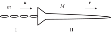
Let us consider a main body which undergoes incremental mass change, increasing (or decreasing) its mass. The mass of this body (subsystem II) and its velocity at an arbitrary instant $t$ are $M$ and ${\bf v}$, respectively, as it is shown in figure 1. The rest of the system (subsystem I) has mass $m$, moving with velocity ${\bf u}$ (${u}>{v}$) at the same instant. So, as the motion progresses the two subsystems I and II coalesce to one another. This means that the body I of mass $m$ loses mass which immediately becomes part of the main body II. We should keep in mind that $m$ and $M$ are time dependent, but the whole system has constant total mass $m+M$, so that mass is being transferred at the rate ${\rm d}\,M/{\rm d}t\,=\,-\,{\rm d}\,m/{\rm d}t$.

Figure 1: Schematic diagram for the two subsystems I and II.

Newton’s second law for the total closed system reads

$${\bf{\cal F}}\,=\,(m\,+M)\,{\bf a}_{\rm cm},$$ (4)

if we adopt the point of view of (2). ${\cal F}$ is the external force acting upon the total system.

The centre of mass velocity is

$${\bf v}_{\rm cm}\,=\,\frac{1}{m+M}\,\left(m\,{\bf u}\,+\,M\,{\bf v}\right).$$ (5)

The time derivative of this expression ($m+M=$ constant, ${\rm d}m/{\rm d}t=-{\rm d}M/{\rm d}t$) is the centre of mass acceleration:

$${\bf a}_{\rm cm}\,=\,\frac{1}{m+M}\,\left(m\,\frac{{\rm d}{\bf u}}{{\rm d}t}\,-\,\frac{{\rm d}M}{{\rm d}t}\,{\bf u}\,+\,M\,\frac{{\rm d}{\bf v}}{{\rm d}t}\,+\,\frac{{\rm d}M}{{\rm d}t}\,{\bf v}\,\right).$$ (6)

The insertion of this expression in (4) led us directly to

$${\bf{\cal F}}\,=\,{\bf F}^{({\rm I})}\,+\,{\bf F}^{({\rm II})}\,=\,m\,\frac{{\rm d}{\bf u}}{{\rm d}t}\,-\,\frac{{\rm d}M}{{\rm d}t}\,{\bf u}\,+\,M\,\frac{{\rm d}{\bf v}}{{\rm d}t}\,+\,\frac{{\rm d}M}{{\rm d}t}\,{\bf v}\,,$$ (7)

where ${\bf F}^{({\rm I})}$ and ${\bf F}^{({\rm II})}$ are the forces acting upon subsystems I and II, respectively.

In order to describe separately the motion of each subsystem I and II, we split (7) into two:

$${\bf F}^{({\rm I})}\,=\,m\,\frac{{\rm d}{\bf u}}{{\rm d}t},\hskip 5.69046pt{\rm for\,the\,variable\,mass\,system\,I,}\,$$ (8)

and

$${\bf F}^{({\rm II})}\,=\,M\,\frac{{\rm d}\,{\bf v}}{{\rm d}\,t}\,+\,({\bf v}\,-\,{\bf u})\,\frac{{\rm d}\,M}{{\rm d}\,t},\hskip 5.69046pt{\rm for\,the\,variable\,mass\,system\,II}\,.$$ (9)

This splitting of (7) into (8) and (9) is physically fruitful as is illustrated in section III.

The role of the systems I and II can be interchanged, and both of them should be described by the standard equation for a variable mass system. With this goal in mind, it is convenient to rewrite (8) and (9) using the linear momentum.

From (8) we obtain

$${\bf F}^{({\rm I})}\,=\,\frac{{\rm d}}{{\rm d}t}\,(m\,{\bf u})\,-\,{\bf u}\,\frac{{\rm d}\,m}{{\rm d}t},$$ (10)

and, from (9),

$${\bf F}^{({\rm II})}\,=\,\frac{{\rm d}}{{\rm d}t}\,(M\,{\bf v})\,-\,{\bf u}\,\frac{{\rm d}\,M}{{\rm d}t},$$ (11)

proving the coherence of the treatment. Both expressions have a common generic structure hence, hereafter, the symbols I or II are dropped.

In conclusion, the standard Newton’s equation of motion for variable mass systems is obtained:

$$\frac{{\rm d}\,{\bf P}}{{\rm d}\,t}\,=\,{\bf F}\,+\,{\bf u}\,\frac{{\rm d}\,M}{{\rm d}\,t}.$$ (12)

It is worth pointing out that:

• the system has instantaneous mass $M$ ($m$), and linear momentum ${\bf P}\,=\,M\,{\bf v}$ ($m\,{\bf u}$);

• ${\bf F}$ is the net external force acting upon the variable mass system;

• ${\bf u}\,{{\rm d}M}/{{\rm d}t}$ (${\bf u}\,{{\rm d}m}/{{\rm d}t}$) is the rate at which momentum is carried into or away from the system of mass $M$ ($m$).

In the present derivation, the definition of the system is clear, as well as the concept of linear momentum which agrees with the concept students are acquainted with. Regarding the approach presented previously, we notice that ${\bf F}$ (see (3)) is the force acting on the whole (constant mass) system.

This approach is suitable for undergraduate students and is equivalent to other methods Tiersten ; MaMa .

III Examples

There are many one-dimensional nonrigid systems, such as chains and ropes, for which the usage of conservation laws of energy and linear momentum represent a good approach. However, the conservation laws always refer to a definite number of particles, although the system under study might be split into two subsystems of variable mass. It is this aspect that is central in our approach. In this context, three illustrative examples are discussed.

III.1 Example 1: Falling of a chain

The upper end of a uniform open-link chain of length $l$, and mass per unit length $\lambda$, is released from rest at $x=0$. The lower end is fixed at point A as it is shown in figure 2. Find the tension $T(x)$ in the chain at point A after the upper end of the chain has dropped the distance $x$. Assume the free fall of the chain.

Figure 2: The chain with the displacement $x$ of the top end.

Solution. According with the suggested methodology, we divide the chain into two parts each to be treated using Newton’s second law for variable mass systems (12). For this purpose we consider:

• subsystem I: the free falling part of the chain, whose mass is $\lambda(l-{x}/{2})$, and velocity $v$;

• subsystem II: the rest of the chain, whose mass is $\lambda\,x/2$, and at rest.

Accordingly, for subsystem I:

$$M\,=\,\lambda\,(l\,-\,\frac{x}{2}),\hskip 14.22636ptP\,=\,\,\lambda\,(l\,-\,\frac{x}{2})\,v,\hskip 14.22636pt{\rm and}\hskip 14.22636ptu=v.$$ (13)

System	$M$	$P$	$F$	$u$	$u\,{\rm d}M/{\rm d}t$
I	$\lambda\,(l\,-\,{x}/{2})$	$\lambda\,(l\,-\,{x}/{2})\,v$	$\lambda\,(l\,-\,{x}/{2})\,g$	$v$	$-\lambda\,v^{2}/2$
II	$\lambda\,\,x/2$	$0$	$\lambda\,x\,g/2+\,T\,(x)$	$v$	$\,\lambda\,v^{2}/2$
I+II	$\lambda\,l$	$\lambda\,(l\,-\,{x}/{2})\,v$	$\lambda\,l\,g+\,T(x)$	—	—

Table 1: Summary of some relevant physical quantities for example 1. See text for notation.

These quantities are displayed in table I, as well as the corresponding quantities for subsystem II and the total system.

As the net external force is $F\,=\,\lambda\,(l\,-\,x/2)\,g$, where $g$ stands for the gravity acceleration, equation (12) can be written as

$$\frac{{\rm d}}{{\rm d}t}\,[\lambda\,(l\,-\,\frac{x}{2})\,v]\,=\,\lambda\,(l\,-\,\frac{x}{2})\,g\,-\,\frac{\lambda}{2}\,v^{2}.$$ (14)

After straightforward simplifications one concludes that $a\,=\,{\rm d}v/{\rm d}t\,=\,g$, which is consistent with the free fall assumption already used to write $F$.

The velocity can then be calculated from ${\rm d}v/{\rm d}t\,=v\,{\rm d}v/{\rm d}x\,=\,g$. The first-order differential equation $v\,{\rm d}v\,-\,g\,{\rm d}x=0$ is integrated ($x_{0}=v_{0}=0$) yielding

$$v\,(x)\,=\,(2\,g\,x)^{1/2}.$$ (15)

As stated above, one can also confirm that a general equation of the type ${\bf F}\,=\,M\,{\bf a}$ applies to subsystem I ($F=\lambda\,(l\,-\,x/2)\,g$, $M=\lambda\,(l\,-\,x/2)$, $a=g$). This is a consequence of having ${v}\,=\,{u}$. In this case mass is being lost but at zero relative velocity.

To proceed, we apply the reasonings used above to subsystem II. As the net external force on this subsystem is $F\,=\,T\,(x)\,+\,\lambda\,x\,g/2$, one finds (see table I), from (12)

$$0\,=\,T\,(x)\,+\,\frac{1}{2}\lambda\,x\,g\,+\,\lambda\,\frac{v^{2}}{2}.$$ (16)

Inserting (15) we obtain for the tension

$$T\,(x)\,=\,-\,\frac{3}{2}\,\lambda\,x\,g.$$ (17)

One may now check this result using (2) for the whole system I+II, and to this end the acceleration of the centre of mass must be obtained.

From figure 2 and table I one has for the centre of mass velocity

$$v_{\rm cm}\,=\,v\,(1\,-\,\frac{x}{2l}).$$ (18)

Taking the time derivative we get the centre of mass acceleration:

$$a_{\rm cm}\,=\,-\,\frac{v^{2}}{2l}\,+\,g\,(1\,-\,\frac{x}{2l}).$$ (19)

Inserting now $v(x)$ as given by (15) in this equation yields

$$a_{\rm cm}\,=\,g\,(1\,-\,\frac{3x}{2l}).$$ (20)

Newton’s second law (2), applied to the chain (closed system I+II), reads (see table I)

$$\lambda\,l\,g\,+\,T\,(x)\,=\,\lambda\,l\,g\,(1\,-\,\frac{3x}{2l}),$$ (21)

which confirms (17) for $T\,(x)$.

This kind of nonrigid systems is also accurate to study energetic processes Sousa . In fact, the initial mechanical energy of the chain is converted into internal energy.

III.2 Example 2: Falling of a rope

A coil of a uniform rope is placed just above a hole in a platform. One end of the rope falls (without friction or air resistance) and pulls down the remaining rope in a steady motion (see figure 3). The rope has total length $l$ and mass per unit length $\lambda$, and starts from rest at $x=0$. Find the normal force $N(x)$ exerted upon the coil, and the tension $T(x)$ in the rope at a distance $x$ from its lower end. The system is confined in a box so that the rope is prevented from lifting up.

Figure 3: Scheme of the rope falling off with $x$ being the length of the rope hanging from the hole.

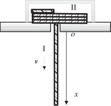
Solution. The rope behaves like a flexible and inextensible one-dimensional conservative system. Under these conditions, as it falls down the mechanical energy is conserved. The acceleration of the falling rope is not known, as well as the forces $N(x)$ and $T(x)$. Notice that these forces, which result from the constraints imposed on the motion of the rope, cannot be specified a priori.

The acceleration of the falling rope may be obtained form the energy conservation.

System	$M$	$P$	$F$	$u$	$u\,{\rm d}M/{\rm d}t$
I	$\lambda\,x$	$\lambda\,x\,v$	$\lambda\,x\,g+\,T(x)$	$v$	$\lambda\,v^{2}$
II	$\lambda\,(l\,-\,x)$	$0$	$\lambda\,(l\,-\,x)\,g+\,N\,(x)\,-\,T(x)$	$v$	$-\,\lambda\,v^{2}$
I+II	$\lambda\,l$	$\lambda\,x\,v$	$\lambda\,l\,g+\,N(x)$	—	—

Table 2: Summary of some relevant physical quantities for example 2. See text for notation.

As illustrated in figure 3, the $x$ axis, whose origin is on the platform, points downwards. The variation of the kinetic energy of the system is

$$\Delta\,K\,(x)\,=\,\frac{1}{2}\,\lambda\,x\,v^{2},$$ (22)

where $v={\rm d}x/{\rm d}t$ is the velocity of the moving part of the rope.

The corresponding variation of the potential energy (whose zero is for $x=0$) is

$$\Delta U(x)\,=\,-\,\frac{1}{2}\,\lambda\,g\,x^{2}.$$ (23)

From the conservation of energy, $\Delta\,E=0$, we obtain the velocity, $v$, as a function of $x$,

$$v(x)\,=\,(g\,x)^{1/2}.$$ (24)

Taking the time derivative of this equation the acceleration of the falling rope is obtained:

$$a\,=\,\frac{{\rm d}v}{{\rm d}t}\,=\,\frac{{\rm d}v}{{\rm d}x}\,\frac{{\rm d}x}{{\rm d}t}\,=\,\frac{g}{2}.$$ (25)

We now illustrate the recommended approach, by looking at the problem from the point of view of a variable mass system.

As figure 3 shows the system at time $t$ can be separated into two subsystems:

• subsystem I: the hanging part with length $x$, mass $\lambda\,x$ and velocity $v$;

• subsystem II: the remainder rope at rest on the platform, with mass $\lambda\,(l-x)$.

Since we are interested to study the rope as a variable mass system, we put it inside a box, as shown in figure 3. Therefore the rope will not depart from the assumed shape as soon as the motion starts.

For subsystem I (see table II, and figure 3) one has:

$$M=\lambda\,x,\hskip 14.22636ptP=\lambda\,x\,v,\hskip 14.22636ptu=v,\hskip 14.22636pt{\rm and}\hskip 14.22636ptu\,\frac{{\rm d}M}{{\rm d}t}\,=\,\lambda\,v^{2}.$$ (26)

Because the external force acting on this system is $F=\lambda\,x\,g\,+\,T(x)$, where $T(x)$ is the tension in the rope at the boundary of subsystem I, (12) leads to

$$\frac{{\rm d}}{{\rm d}t}\,(\lambda\,x\,v)\,=\,\lambda\,x\,g\,+\,T(x)\,+\,\lambda\,v^{2},$$ (27)

and, after using (25),

$$T\,(x)\,=\,\lambda\,x\,(a\,-\,g)\,=\,-\,\frac{1}{2}\lambda\,x\,g.$$ (28)

As we have already said, a general equation of the type ${\bf F}\,=\,M\,{\bf a}$ is also valid for this part of the system ($F\,=\,\lambda\,x\,g/2$, $M=\lambda\,x$, $a={\rm d}v/{\rm d}t\,=\,g/2$). As in example 1, also here the mass is acquired at zero relative velocity.

A similar study for subsystem II can be carried out. The relevant physical quantities for this variable mass system are also given in table II.

As the net external force on subsystem II includes the weight of part of the rope, $\lambda\,(l\,-\,x)\,g$, the tension, $-\,T\,(x)\,=\,\lambda\,x\,g/2$, and the total force by the platform, $N(x)$, the equation of motion (12) yields

$$0\,=\,\lambda\,(l\,-\,x)\,g\,+\frac{1}{2}\,\lambda\,x\,g\,+\,\,N\,(x)\,-\,\lambda\,v^{2}.$$ (29)

Using (24) the normal force on the rope can be obtained:

$$N\,(x)\,=-\lambda\,(l\,-\,\frac{3}{2}\,x)\,g,$$ (30)

showing that $N(x)=0$ when $x=2l/3$. We may now confirm this result by applying Newton’s second law to the closed system I+II using (2).

The velocity of the centre of mass can be calculated directly from the quantities mentioned in figure 3 and in table II:

$$v_{\rm cm}\,=\,\frac{x}{l}\,v\,=\,\frac{x}{l}\,(g\,x)^{1/2}.$$ (31)

The time derivative of this equation, together with (24) and (25), allows us calculate the acceleration of the centre of mass

$$a_{\rm cm}\,=\,\frac{{\rm d}\,v_{\rm cm}}{{\rm d}\,t}\,=\,\frac{v^{2}}{l}\,+\,\frac{x}{l}\,a\,=\,g\,\frac{3\,x}{2\,l}.$$ (32)

This equation shows that $a_{\rm cm}$ becomes equal to $g$ when $x=2\,l/3$, and agrees with $N\,(x)\,=\,0$ for that value of $x$.

Newton’s second law (2) applied to the system I+II (see table II) leads to

$$\lambda\,l\,g\,+\,N\,(x)\,=\,\lambda\,l\,(\,\frac{3\,x}{2\,l}\,g),$$ (33)

resulting a total force on the rope as given by (30), showing the validity of the suggested method.

III.3 Example 3: Pulling a rope

A uniform rope, of length $l$ and mass per unit length $\lambda$, is pulled along a smooth horizontal surface by a constant force $F$. Find the tension in the rope at any point a distance $x$ from the end where $F$ is applied.

Figure 4: Configuration of the rope being pulled on a smooth horizontal surface by the constant force $F$.

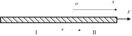
Solution. Using again the variable mass problem-solving perspective, we present in table III (see also figure 4) some of the relevant physical quantities for this example. The origin of the reference system is such that $x$ is the coordinate of the point of application of $F$.

The equation of motion (12), applied to subsystem I, is written as

$$\frac{{\rm d}}{{\rm d}t}\,[\lambda\,(l\,-\,x)\,v]\,=\,T\,(x)\,-\,\lambda\,v^{2},$$ (34)

where $T(x)$ is the tension in the rope at a distance $x$ from the front top of the rope. The terms involving the velocity cancel in both sides of (34) and therefore

$$T\,(x)\,=\,\lambda\,(l\,-\,x)\,a,$$ (35)

where $a$ is the acceleration of the rope.

System	$M$	$P$	$F$	$u$	$u\,{\rm d}M/{\rm d}t$
I	$\lambda\,(l\,-\,x)$	$\lambda\,(l\,-\,x)\,v$	$T(x)$	$v$	$-\,\lambda\,v^{2}$
II	$\lambda\,x$	$\lambda\,x\,v$	$F\,-\,T(x)$	$v$	$\,\lambda\,v^{2}$
I+II	$\lambda\,l$	$\lambda\,l\,v$	$F$	—	—

Table 3: Summary of relevant physical quantities for example 3. See text for notation.

Regarding subsystem II, we obtain, from (12)

$$\frac{{\rm d}}{{\rm d}t}\,(\lambda\,x\,v)\,=\,-\,T\,(x)\,+\,F\,+\,\lambda\,v^{2}.$$

Using (35) in this equation the acceleration turns out to be $a=F/(\lambda\,l)$. Finally, inserting this acceleration into (35), we obtain

$$T\,(x)\,=\,F\,(1\,-\,\frac{x}{l}\,),$$ (36)

allowing for the correct limits $T\,(x=0)\,=\,F$ and $T\,(x=l)\,=\,0$.

Since we have now $u=v$ for both subsystems, a general equation of type (2) (see also (8) and (9)) could be used directly, leading to the correct results.

In this context, as already pointed out by Tiersten Tiersten using the concept of flux, equation (1) could not be used to obtain the tension $T(x)$. In fact, choosing, for instance, the subsystem I we have: $F\,=\,T\,(x)$, $dP/dt\,=\,-\,\lambda\,v^{2}\,+\,\lambda\,(l\,-\,x)\,a$, which does not lead to the correct expression for $T(x)$.

IV Conclusions

In this paper we suggested a method suitable for discussing variable mass systems in a straightforward way, and presented three applications. Usually the study of the systems under consideration is elaborated over a fixed number of particles, and so both forms of Newton’s second law, either ${\bf F}\,=\,M\,{\bf a}$ or ${\bf F}\,=\,{\rm d}\,{\bf P}/{\rm d}t$, can be used Siegel ; Sousa .

So far as the question of the validity of multi-particle forms of Newton’second law is concerned, three special cases must be considered:

• $M\,=\,{\rm constant}$ (in this case ${\bf F}\,=\,{{\rm d}\,{\bf P}}/{{\rm d}\,t}$ and ${\bf F}\,=\,M\,{\bf a}$ are equivalent);

• ${\bf u}=0$, i.e. the increment of mass ${\rm d}\,M$ is at rest;

  and

• ${\bf u}\,=\,{\bf v}$.

So, as the general equation (12) shows, ${\bf F}\,=\,{{\rm d}\,{\bf P}}/{{\rm d}\,t}$ is the correct equation of motion only in two special cases (i) and (ii). For example, the raindrop falling through a stationary cloud of droplets Krane inserts into the case (ii). In general, as the present illustrative examples show, conditions (i) and (ii) above are not satisfied and, consequently, ${\bf F}\,=\,{{\rm d}\,{\bf P}}/{{\rm d}\,t}$ does not provide the equation of motion of the corresponding subsystems I and II.

On the other hand, if the case (iii) applies, a general equation of the type ${\bf F}\,=\,M\,{\bf a}$ can be used (see (9)). Referring, in particular, to example 3, since in this case ${\bf v}\,=\,{\bf u}$ for both subsystems, they can be solved by such a general equation.The same considerations apply to subsystem I of the other examples. However, let us stress that this does not mean that this form of the Newton’s second law is more fundamental than (1) in the context of classical mechanics, and that care must be taken when referring to variable mass systems.

Acknowledgments

Work supported by FCT. We would like to thank M. C. Ruivo, L. Brito and A. Blin for fruitful discussions. We are also grateful to M. Fiolhais for a careful reading of the manuscript and helpful suggestions.

References

- (1) J. F. Thorpe, ”On the momentum theorem for a continuous system of variable mass”, Am. J. Phys. 30, 637-640 (1962).
- (2) A. B. Arons and A. M. Bork, ”Newton’s laws of motion and the 17th century laws of impact”, Am. J. Phys. 32, 313-317 (1964).
- (3) M. Tiersten, ”Force, momentum change, and motion”, Am. J. Phys. 37, 82-87 (1969).
- (4) S. Siegel, ”More about variable mass systems”, Am. J. Phys. 67, 1063-1067 (1972).
- (5) K. S. Krane, ”The falling raindrop: Variations on a theme of Newton”, Am. J. Phys. 49, 113-117 (1981).
- (6) H. Benson, University Physics (Wiley, New York, 1996), revised ed. pp. 204-205
- (7) J. Matolyak and G. Matous, ”Simple variable mass systems: Newton’s second law”, The Phys. Teach. 28, 328-329 (1990).
- (8) C. A. de Sousa, ”Nonrigid systems: mechanical and thermodynamic aspects”, Eur. J. Phys. 23, 433-440 (2002).