Broad distribution effects in sums of lognormal random variables

Abstract

The lognormal distribution describing, e.g., exponentials of Gaussian random variables is one of the most common statistical distributions in physics. It can exhibit features of broad distributions that imply qualitative departure from the usual statistical scaling associated to narrow distributions. Approximate formulae are derived for the typical sums of lognormal random variables. The validity of these formulae is numerically checked and the physical consequences, e.g., for the current flowing through small tunnel junctions, are pointed out.

I Introduction: physics motivation

Most usual phenomena present a well defined average behaviour with fluctuations around the average values. Such fluctuations are described by narrow (or ’light-tailed’) distributions like, e.g., Gaussian or exponential distributions. Conversely, for other phenomena, fluctuations themselves dictate the main features, while the average values become either irrelevant or even non existent. Such fluctuations are described by broad (or ’heavy-tailed’) distributions like, e.g., distributions with power law tails generating ’Lévy flights’. After a long period in which the narrow distributions have had the quasi-monopoly of probability applications, it has been realized in the last fifteen years that broad distributions arise in a number of physical systems Bouchaud and Georges (1990); Shlesinger et al. (1995); Kutner et al. (1999).

Macroscopic physical quantities often appear as the sums $S_{n}$ of microscopic quantities $x_{i}$:

$$S_{n}=\sum_{i=1}^{n}x_{i},$$ (1)

where $x_{1},x_{2},\ldots,x_{n}$ are independent and identically distributed random variables. The dependence of such sums $S_{n}$ with the number $n$ of terms epitomizes the role of the broadness of probability distributions of $x_{i}$’s. One intuitively expects the typical sum $S_{n}^{\mathrm{t}}$ to be given by:

$$S_{n}^{\mathrm{t}}\simeq n\langle x\rangle,$$ (2)

where $\langle x\rangle$ is the average value of $x$. The validity of eq. (2) is guaranteed at large $n$ by the law of large numbers. However, the law of large numbers is only valid for sufficiently narrow distributions. Indeed, for broad distributions, the sums $S_{n}$ can strongly deviate from eq. (2). For instance, if the distribution of the $x_{i}$’s has a power law tail (cf. Lévy flights, Bouchaud and Georges (1990)), $\propto 1/x^{1+\alpha}$ with $0<\alpha<1$ ($\langle x\rangle=\infty$), then the typical sum of $n$ terms is not proportional to the number of terms but is given by:

$$S_{n}^{\mathrm{t}}\propto n^{1/\alpha}.$$ (3)

Physically, eq. (2) (narrow distributions) and eq. (3) (Lévy flights) correspond to different scaling behaviours. For the Lévy flight case, the violation of the law of large numbers occurs for any $n$. On the other hand, for other broad distributions like the lognormal treated hereafter, there is a violation of the law of large numbers only for finite, yet surprisingly large, $n$’s.

These violations of the law of large numbers, whatever their extent, correspond physically to anomalous scaling behaviours as compared to those generated by narrow distributions. This applies in particular to small tunnel junctions, such as the metal-insulator-metal junctions currently studied for spin electronics Moodera et al. (1995); Miyazaki and Tezuka (1995). It has indeed been shown, theoretically Bardou (1997) and experimentally Costa et al. (2000a); Kelly (1999), that these junctions tend to exhibit a broad distribution of tunnel currents that generates an anomalous scaling law: the typical integrated current flowing through a junction is not proportional to the area of the junction. This is more than just a theoretical issue since this deviation from the law of large numbers is most pronounced Costa et al. (2000a, 2002) for submicronic junction sizes relevant for spin electronics applications.

A similar issue is topical for the future development of metal oxide semiconductor field effect transistors (MOSFETs). Indeed, the downsizing of MOSFETs requires a reduction of the thickness of the gate oxide layer. This implies that tunnelling through the gate becomes non negligibleCassan et al. (1999); Momose et al. (1998), generating an unwanted current leakage. Moreover, as in metal-insulator-metal junctions, the large fluctuations of tunnel currents may give rise to serious irreproducibility issues. Our model permits a statistical description of tunnelling through non ideal barriers applying equally to metal-insulator-metal junctions and to MOSFET current leakages. Thus, anomalous scaling effects are expected to arise also in MOSFETs.

The current fluctuations in tunnel junctions are well described by a lognormal probability density Costa et al. (1998, 2000a)

$$f(x)=\mathrm{LN}(\mu,\sigma^{2})(x)=\frac{1}{\sqrt{2\pi\sigma^{2}}x}\exp\left[-\frac{\left(\ln x-\mu\right)^{2}}{2\sigma^{2}}\right],x>0$$ (4)

depending on two parameters, $\mu$ and $\sigma^{2}$. The lognormal distribution presents at the same time features of a narrow distribution, like the finiteness of all moments, and features of a broad distribution, like a tail that can extend over several decades. It is actually one of the most common statistical distributions and appears frequently, for instance, in biology Limpert et al. (2001) and finance Bouchaud and Potters (2000) (for review see Crow and Shimizu (1988); Aitchinson and Brown (1957)). In physics, it is often found in transport through disordered systems such as wave propagation in random media (radar scattering, mobile phones,…)Schwartz and Yeh (1982); Beaulieu et al. (1995). A specially relevant example of the latter is transport through 1D disordered insulating wires for which the distribution of elementary resistances has been shown to be lognormal Ladieu and Bouchaud (1993). This wire problem of random resistances in series is equivalent to the tunnel junction problem of random conductances in parallel Raĭkh and Ruzin (1989). Thus, our results, initially motivated by sums of lognormal conductances in tunnel junctions, are also relevant for sums of lognormal resistances in wires.

In this paper, our aim is to obtain analytical expressions for the dependence on the number $n$ of terms of the typical sums $S_{n}^{\mathrm{t}}$ of identically distributed lognormal random variables. The theory must treat the $n$ and $\sigma^{2}$ ranges relevant for applications. For tunnel junctions, both small $n\simeq 1$ corresponding to nanometric sized junctions Costa et al. (1998) and large $n\simeq 10^{13}$ corresponding to millimetric sized junctions, and both small $\sigma^{2}\simeq 0.1$ and large $\sigma^{2}\simeq 10$ Dimopoulos (2002); Costa et al. (2000b); Dimopoulos et al. (2001); Costa et al. (2000a) have been studied experimentally. For electromagnetic propagation in random media, $\sigma^{2}$ is typically in the range 2 to 10 Beaulieu et al. (1995).

There exist recent mathematical studies on sums of lognormal random variables Arous et al. (2002); Bovier et al. (2002) that are motivated by glass physics (Random Energy Model). However, these studies apply to regimes of large $n$ and/or large $\sigma^{2}$ that do not correspond to those relevant for our problems. Our work concentrates on the deviation of the typical sum of a moderate number of lognormal terms with $\sigma^{2}\lesssim 15$ from the asymptotic behaviour dictated by the law of large numbers. Thus, this paper and Arous et al. (2002); Bovier et al. (2002) treat complementary $\left(n,\sigma^{2}\right)$ ranges.

Section II is a short review of the basic properties of lognormal distributions, insisting on their broad character. Section III presents qualitatively the sums of $n$ lognormal random variables. Section IV introduces the strategies used to estimate the typical sum $S_{n}^{\mathrm{t}}$. Section V, the core of this work, derives approximate analytical expressions of $S_{n}^{\mathrm{t}}$ for different $\sigma^{2}$-ranges. Section VI discusses the range of validity of the obtained results. Section VII presents the striking scaling behaviour of the sample mean inverse. Section VIII contains a summarizing table and an overview of main results.

As the paper is written primarily for practitioners of quantum tunnelling, it reintroduces in simple terms the needed statistical notions about broad distributions. However, most of the paper is not specific to quantum tunnelling and its results may be applied to any problem with sums of lognormal random variables. The adequacy of the presented theory to describe experiments on tunnel junctions is presented in Costa et al. (2002).

II The lognormal distribution: simple properties and narrow vs broad character

In this section, we present simple properties (genesis, characteristics, broad character) of the lognormal distribution that will be used in the next sections.

Among many mechanisms that generate lognormal distributions Crow and Shimizu (1988); Aitchinson and Brown (1957), two of them are especially important in physics. In the first generation mechanism, we consider $x$ as exponentially dependent on a Gaussian random variable $y$ with mean $\mu_{y}$ and variance $\sigma_{y}^{2}$:

$$x=x_{0}e^{y/y_{0}}$$ (5)

where $x_{0}$ and $y_{0}$ are scale parameters for $x$ and $y$, respectively. The probability density of $y$ is:

$$\mathrm{N}(\mu_{y},\sigma_{y}^{2})(y)=\frac{1}{\sqrt{2\pi\sigma_{y}^{2}}}\exp\left[-\frac{\left(y-\mu_{y}\right)^{2}}{2\sigma_{y}^{2}}\right].$$ (6)

The probability density of $x$, $f(x)=\mathrm{N}(\mu_{y},\sigma_{y}^{2})(y){\mathrm{d}}{y}/{\mathrm{d}}{x}$ is a lognormal density $\mathrm{LN}\left(\mu,\sigma^{2}\right)\left(x\right)$, as in eq. (4), with parameters:

$$\mu=\frac{\mu_{y}}{y_{0}}+\ln{x_{0}},$$ (7a)

$$\sigma^{2}=\left(\sigma_{y}/y_{0}\right)^{2}.$$ (7b)

A typical example of such a generation mechanism is provided by tunnel junctions. Indeed, the exponential current dependence on the potential barrier parameters operates as a kind of ’fluctuation amplifier’ by non-linearly transforming small Gaussian fluctuations of the parameters into qualitatively large current fluctuations. This implies, as seen above, lognormal distribution of tunnel currents Costa et al. (2002).

In the second generation mechanism, we consider the product $x_{n}=\prod_{i=1}^{n}{y_{i}}$ of $n$ identically distributed random variables $y_{1},\cdots,y_{n}$. If $\mu^{\prime}$ and $\sigma^{\prime}$ are the mean and the standard deviation of $\ln{y_{i}}$, not necessarily Gaussians, then

$$\ln{x_{n}}=\sum_{i=1}^{n}{\ln{y_{i}}}$$ (8)

tends, at large $n$, to a Gaussian random variable of mean $n\mu^{\prime}$ and variance $n\sigma{{}^{\prime}}^{2}$, according to the central limit theorem. Hence, using eqs. (7a) and (7b) with $x_{0}=y_{0}=1$, $x_{n}$ is lognormally distributed with parameters $\mu=n\mu^{\prime}$ and $\sigma^{2}=n\sigma{{}^{\prime}}^{2}$. For a better approximation at finite $n$, see Redner (1990).

The lognormal distribution given by eq. (4) has the following characteristics.

The two parameters $\mu$ and $\sigma^{2}$ are, according to eq. (7a) and eq. (7b) with $x_{0}=y_{0}=1$, the mean and the variance of the Gaussian random variable $\ln x$. The parameter $\mu$ is a scale parameter. Indeed, if $x$ is distributed according to $\mathrm{LN}(\mu,\sigma^{2})(x)$, then $x^{\prime}=\alpha x$ is distributed according to $\mathrm{LN}(\mu^{\prime}=\mu+\ln\alpha,{\sigma^{\prime}}^{2}=\sigma^{2})(x^{\prime})$, as can be seen from eq. (5), eq. (7a) and eq. (7b). Thus, one can always take $\mu=0$ using a suitable choice of units. On the other hand, $\sigma^{2}$ is the shape parameter of the lognormal distribution.

The typical value $x^{\mathrm{t}}$, corresponding to the maximum of the distribution, is

$$x^{\mathrm{t}}=e^{\mu-\sigma^{2}}.$$ (9)

The median, ${x^{\mathrm{m}}}$, such that $\int_{0}^{x^{\mathrm{m}}}f(x){\mathrm{d}}x=\int_{x^{\mathrm{m}}}^{\infty}f(x){\mathrm{d}}x=1/2$, is

$${x^{\mathrm{m}}}=e^{\mu}.$$ (10)

The average, $\langle x\rangle$, and the variance, ${\mathrm{var}}\left(x\right)\equiv\langle x^{2}\rangle-\langle x\rangle^{2}$, are

$$\langle x\rangle = e^{\mu+\sigma^{2}/2},$$ (11)

$${\mathrm{var}}\left(x\right) = e^{2\mu+\sigma^{2}}\left(e^{\sigma^{2}}-1\right).$$ (12)

The coefficient of variation, $C\equiv\sqrt{{\mathrm{var}}\left(x\right)}/\langle x\rangle$, which characterizes the relative dispersion of the distribution, is thus

$$C=\sqrt{e^{\sigma^{2}}-1}.$$ (13)

Note that $\mu$ does not appear in $C$, as expected for a scale parameter.

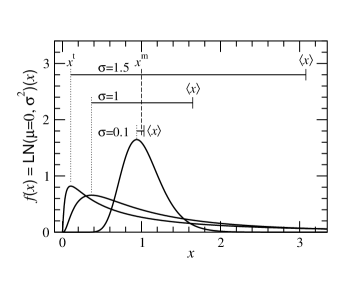
Figure 1: Examples of lognormal distributions $\mathrm{LN}\left(\mu,\sigma^{2}\right)\left(x\right)$ with $\mu=0$ and $\sigma=$ 0.1, 1 and 1.5. When $\sigma$ increases, the typical values $x^{\mathrm{t}}$, indicated by the dotted lines, and the means $\langle x\rangle$ move rapidly away from the constant median ${x^{\mathrm{m}}}$, indicated by the broken line, in opposite directions.

Figure 1 shows examples of lognormal distributions with scale parameter $\mu=0$ and different shape parameters. For small $\sigma^{2}$, the lognormal distribution is narrow (rapidly decaying tail) and can be approximated by a Gaussian distribution (see Appendix A). When $\sigma^{2}$ increases, the lognormal distribution rapidly becomes broad (tail extending to values much larger than the typical value). In particular, the typical value $x^{\mathrm{t}}$ and the mean $\langle x\rangle$ move in opposite directions away from the median ${x^{\mathrm{m}}}$ which is 1 for all $\sigma^{2}$. The strong $\sigma^{2}$-dependence of the broadness is quantitatively given by the coefficient of variation, eq. (13).

Another way of characterizing the broadness of a distribution, is to define an interval containing a certain percentage of the probability. For the Gaussian distribution $\mathrm{N}\left(\mu,\sigma^{2}\right)$, 68% of the probability is contained in the interval $\left[\mu-\sigma,\mu+\sigma\right]$ whereas for the lognormal distribution $\mathrm{LN}\left(\mu,\sigma^{2}\right)$, the same probability is contained within $\left[{x^{\mathrm{m}}}/e^{\sigma},{x^{\mathrm{m}}}\times e^{\sigma}\right]$. The extension of this interval depends linearly on $\sigma$ for the Gaussian and exponentially for the lognormal.

Moreover, the weighted distribution $xf\left(x\right)$, giving the distribution of the contribution to the mean, is peaked on the median ${x^{\mathrm{m}}}$. In the vicinity of ${x^{\mathrm{m}}}$ one hasMontroll and Shlesinger (1983):

$$f(x)=\frac{1}{\sqrt{2\pi\sigma^{2}}x}~{}\mathrm{for}~{}e^{\mu-\sqrt{2}\sigma}\ll x\ll e^{\mu+\sqrt{2}\sigma}.$$ (14)

Thus, $f\left(x\right)$ behaves as a distribution that is extremely broad ($1/x$ is not even normalizable) in an $x$-interval whose size increases exponentially fast with $\sigma$ and that is smoothly truncated outside this interval.

Three different regimes of broadness can be defined using the peculiar dependence of the probability peak height $f\left(x^{\mathrm{t}}\right)$ on $\sigma^{2}$. Indeed, the use of eq. (4) and eq. (9) yields:

$$f(x^{\mathrm{t}})=\frac{e^{\sigma^{2}/2}}{\sqrt{2\pi}e^{\mu}\sigma}.$$ (15)

For $\sigma^{2}\ll 1$, one has $f(x^{\mathrm{t}})\propto 1/\sigma$ and thus $f(x^{\mathrm{t}})\propto 1/\sqrt{{\mathrm{var}}\left(x\right)}$ as $\sqrt{{\mathrm{var}}\left(x\right)}\propto\sigma$ (see eq. (12)). This inverse proportionality between peak height $f(x^{\mathrm{t}})$ and peak width $\sqrt{{\mathrm{var}}\left(x\right)}$ is the usual behaviour for a narrow distribution that concentrates most of the probability into the peak.

When the shape parameter $\sigma^{2}$ increases, still keeping $\sigma^{2}\leq 1$, $f(x^{\mathrm{t}})$ is no longer inversely proportional to $\sqrt{{\mathrm{var}}\left(x\right)}$, however it still decreases, as expected for a distribution that becomes broader and thus less peaked (see, in figure 1, the difference between $\sigma=0.1$ and $\sigma=1$).

On the contrary, when $\sigma^{2}>1$, the peak height increases with $\sigma^{2}$ even though the distribution becomes broader (see, in figure 1, the difference between $\sigma=1$ and $\sigma=1.5$). This is more unusual. The behaviour of the peak can be understood from the genesis of the lognormal variable $x=e^{y}$ with $y$ distributed as $\mathrm{N}\left(\mu_{y}=\mu,\sigma_{y}^{2}=\sigma^{2}\right)\left(y\right)$. When $\sigma^{2}$ becomes larger, the probability to draw $y$ values much smaller than $\mu$ increases, yielding many $x$ values much smaller than $e^{\mu}$, all packed close to $0$. This creates a narrow and high peak for $f(x)$.

This non monotonous variation of the probability peak $f(x^{\mathrm{t}})$ with the shape parameter $\sigma^{2}$ with a minimum in $\sigma^{2}=1$, incites to consider three qualitative classes of lognormal distributions, that will be used in the next sections. The class $\sigma^{2}\ll 1$ corresponds to the narrow lognormal distributions that are approximately Gaussian. The class $\sigma^{2}\lesssim 1$ contains the moderately broad lognormal distributions that may deviate significantly from Gaussians, yet retaining some features of narrow distributions. The class $\sigma^{2}\gg 1$ contains the very broad lognormal distributions.

III Qualitative behaviour of the typical sum of lognormal random variables

In this section we explain the qualitative behaviour of the typical sum of lognormal random variables by relating it to the behaviours of narrow and broad distributions.

Consider first a narrow distribution $f_{\mathrm{N}}(x)$ presenting a well defined narrow peak concentrating most of the probability in the vicinity of the mean $\langle x\rangle$ and with light tails decaying sufficiently rapidly away from the peak (figure 2a). Draw, for example, three random numbers $x_{1}$, $x_{2}$ and $x_{3}$ according to the distribution $f_{\mathrm{N}}(x)$. If $f_{\mathrm{N}}(x)$ is sufficiently narrow, then $x_{1}$, $x_{2}$ and $x_{3}$ will all be approximately equal to each other and to the mean $\langle x\rangle$ and thus,

$$S_{3}=x_{1}+x_{2}+x_{3}\simeq 3x_{1,\,2\,\mathrm{or}\,3}\simeq 3\langle x\rangle.$$ (16)

Note that no single term $x_{i}$ dominates the sum $S_{3}$. More generally, the sum of $n$ terms will be close, even for small $n$’s, to the large $n$ expression given by the law of large numbers:

$$S_{n}\simeq n\langle x\rangle.$$ (17)

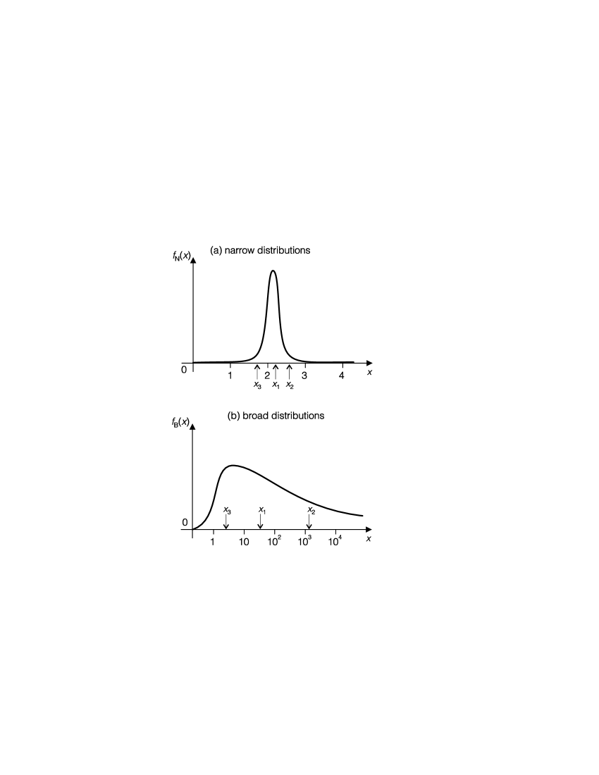
Figure 2: Narrow vs broad distributions. (a) A narrow distribution $f_{\mathrm{N}}(x)$ presents a well defined peak and light tails. In a set $\{x_{1},\ldots,x_{n}\}$ of $n$ random numbers drawn from $f_{\mathrm{N}}(x)$, no number is dominant. (b) A broad distribution $f_{\mathrm{B}}(x)$ presents a long tail extending over several decades (note the logarithmic $x$-scale). In a set $\{x_{1},\ldots,x_{n}\}$ of $n$ random numbers drawn from $f_{\mathrm{B}}(x)$, one number is clearly dominant.

Consider now a broad distribution $f_{\mathrm{B}}(x)$ whose probability spreads throughout a long tail extending over several decades (figure 2b; note the logarithmic $x$-scale) instead of being concentrated into a peak. Drawing three random numbers according to $f_{\mathrm{B}}(x)$, it is very likely that one of these numbers, for example $x_{2}$, will be large enough, compared to the other ones, to dominate the sum $S_{3}$:

$$S_{3}=x_{1}+x_{2}+x_{3}\simeq\max(x_{1},x_{2},x_{3})=x_{2}.$$ (18)

More generally, the largest term $M_{n}$,

$$M_{n}\equiv\max(x_{1},\ldots,x_{n}),$$ (19)

will dominate the sum of $n$ terms:

$$S_{n}\simeq M_{n}.$$ (20)

Under these premises, what is the order of magnitude of $S_{n}$? To approximately estimate it, one can divide the interval $[0;\infty)$ of possible values of $x$ into $n$ intervals $[a_{1}=0;a_{2})$, $[a_{2};a_{3})$, …, $[a_{n};a_{n+1}=\infty)$ corresponding to a probability of $1/n$:

$$\frac{1}{n}=\int_{a_{j}}^{a_{j+1}}f_{\mathrm{B}}(x)\;{\mathrm{d}}x\,.$$ (21)

Intuitively, there is typically one random number $x_{i}$ in each interval $[a_{j};a_{j+1})$. The largest number $M_{n}$ is thus very likely to lie in the rightmost interval $[a_{n};\infty)$. The most probable number in this interval is $a_{n}$ (we assume that $f_{\mathrm{B}}(x)$ is decreasing at large $x$). Thus, applying eq. (20) the sum $S_{n}$ is approximately given by:

$$S_{n}\simeq a_{n}\ \mathrm{with}\ \frac{1}{n}=\int_{a_{n}}^{\infty}f_{\mathrm{B}}(x)\;{\mathrm{d}}x.$$ (22)

As a specific application, consider for example a Pareto distribution $f_{\mathrm{P}}(x)$ with infinite mean,

$$f_{\mathrm{P}}(x)\equiv\frac{\alpha x_{0}^{\alpha}}{x^{1+\alpha}},\quad\mathrm{for}\quad x\geq x_{0}\quad\mathrm{and}\quad\mathrm{with}\quad 0<\alpha<1.$$ (23)

In this case, the sum $S_{n}$ is called a ’Lévy flight’. The relation  (22) yields $M_{n}^{\mathrm{t}}\simeq x_{0}n^{1/\alpha}$ and thus, using eq. (20),

$$S_{n}^{\mathrm{t}}\simeq x_{0}n^{1/\alpha}.$$ (24)

Note that, as $\alpha<1$, the average value is infinite and thus the law of large numbers does not apply here.

The fact that the sum $S_{n}$ of $n$ terms increases typically faster in eq. (24) than the number $n$ of terms is in contrast with the law of large numbers. This ’anomalous’ behaviour can be intuitively explained (see also figure 3 in Costa et al. (2002) for a complementary approach). Each draw of a new random number from a broad distribution $f_{\mathrm{B}}(x)$ gives the opportunity to obtain a large number, very far in the tail, that will dominate the sum $S_{n}$ and will push it towards significantly larger values. Conversely, for narrow distributions $f_{\mathrm{N}}(x)$, the typical largest term $M_{n}^{\mathrm{t}}$ increases very slowly with the number of terms (e.g., as $\sqrt{\ln n}$ for a Gaussian distribution and as $\ln n$ for an exponential distribution; see, e.g., Embrechts et al. (1997)), whilst the typical sum $S_{n}^{\mathrm{t}}$ increases linearly with $n$ and thus $S_{n}^{\mathrm{t}}\gg M_{n}^{\mathrm{t}}$.

The question that arises now is whether the sum of lognormal random variables behaves like a narrow or like a broad distribution. On one hand, the lognormal distribution has finite moments, like a narrow distribution. Therefore, the law of large numbers must apply at least for an asymptotically large number of terms: $S_{n}\mathrel{\mathop{\kern 0.0pt\to}\limits_{n\to\infty}}n\langle x\rangle$. On the other hand, if $\sigma^{2}$ is sufficiently large, the lognormal tail extends over several decades, as for a broad distribution (see Section II). Therefore, the sum of $n$ terms is expected to be dominated by a small number of terms, if $n$ is not too large.

The domination of the sum by the largest terms can be quantitatively estimated by computing the relative contribution $p_{q}$ to the mean by the proportion $q$ of statistical samples with values larger than some $x_{q}$

$$p_{q}\equiv\int_{x_{q}}^{\infty}x^{\prime}f(x^{\prime}){\mathrm{d}}x^{\prime}/\langle x\rangle,$$ (25)

$$q\equiv\int_{x_{q}}^{\infty}f(x^{\prime}){\mathrm{d}}x^{\prime}.$$ (26)

Figure 3a shows a plot of $p_{q}$ vs $q$ for various $\sigma$’s. Note that the curve $\left(1-q,1-p_{q}\right)$ is called a Lorenz plot in the economics community when studying the distribution of incomes (see, e.g., Drăgulescu and Yakovenko (2001)). For small $\sigma$’s ($\sigma\lesssim 0.25$), one has $p_{q}\simeq q$ for all $q$: all terms $x_{i}$ equally contribute to the sum $S_{n}$. This is the usual behaviour of a narrow distribution. For larger $\sigma$’s, one has $p_{q}\gg q$ for $q\ll 1$: only a small number of terms contribute significantly to the sum $S_{n}$. This is the usual behaviour of a broad distribution. Monte Carlo simulations of tunnelling through MOSFET gates yield $p_{q}$ vs $q$ curves that are strikingly similar to figure 3a (see figure 11 of Cassan et al. (1999)). Indeed, the parameters used in Cassan et al. (1999) correspond to a barrier thickness standard deviation of $\sigma_{d}=0.18\ \mathrm{nm}$, a barrier penetration length $\lambda\simeq 7.8\times 10^{-2}\ \mathrm{nm}$ which gives $\sigma=\sigma_{d}/\lambda\simeq 2.3$ (see Costa et al. (2000a) or Costa et al. (2002) for the derivation of $\sigma=\sigma_{d}/\lambda$). For this $\sigma$, figure 11 of Cassan et al. (1999) fits our $p_{q}$ vs $q$ without any adjustable parameter.

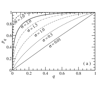
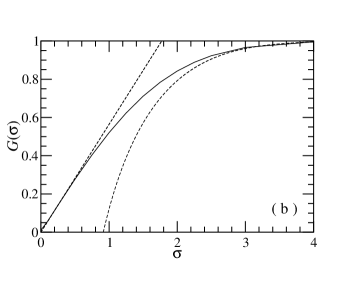
Figure 3: Heterogeneity of the terms of lognormal sums. a) Average proportion $p_{q}$ of the average physical quantity $\langle x\rangle$ carried by the average proportion $q$ of the statistical sample. For narrow lognormal distributions $\left(\sigma^{2}\ll 1\right)$, all terms equally contribute to the sums $\left(p_{q}\simeq q\right)$. For broad lognormal distributions, a small proportion of the terms provide the major contribution to the sums $\left(p_{q}\gg q\mathrm{\ for\ }q\ll 1\right)$. b) Gini coefficient giving a quantitative measure of the heterogeneity.

As in economics, the information contained in figure 3a can be summarized by the Gini coefficient $G$ represented in figure 3b:

$$G\equiv 2\int_{0}^{1}\left(p_{q}-q\right){\mathrm{d}}q,$$ (27)

giving a quantitative measure of the heterogeneity of the contribution of the terms to the sum. In the lognormal case this expression becomes: $G\left(\sigma\right)=1-2\int_{-\infty}^{\infty}\mathrm{N}\left(0,1\right)\left(u\right)\Phi\left(u-\sigma\right){\mathrm{d}}u$, where $\mathrm{N}\left(0,1\right)\left(u\right)$ is the normal distribution (eq. (6)) and $\Phi\left(u\right)\equiv\int_{-\infty}^{u}\mathrm{N}\left(0,1\right)\left(u^{\prime}\right){\mathrm{d}}u^{\prime}$ the corresponding distribution function. The solid line in figure 3b represents $G\left(\sigma\right)$ for various $\sigma$’s. As expected, $G\left(\sigma\right)$ varies from 0 when $\sigma=0$, which means that all terms of a narrow lognormal distribution equally contribute to the sums, to 1 when $\sigma\to\infty$, which means that only a small proportion of the terms of a broad lognormal distribution contributes significantly to the sums. The broken lines in figure 3b represent analytically derived asymptotic approximations of $G\left(\sigma\right)$:

$$\sigma\ll 1:G\left(\sigma\right)\simeq\frac{\sigma}{\sqrt{\pi}}$$ (28a)

$$\sigma\gg 1:G\left(\sigma\right)\simeq 1-\frac{2e^{-\sigma^{2}/4}}{\sqrt{\pi}\sigma}$$ (28b)

(Our derivations of these formulae, which are not explicitely shown here, are based on usual expansion techniques).

In summary, if $\sigma^{2}$ is small, the sum of $n$ lognormal terms is expected to behave like sums of narrowly distributed random variables, for any $n$. Conversely, if $\sigma^{2}$ is sufficiently large, the sum of $n$ lognormal terms is expected to behave, at small $n$, like sums of broadly distributed random variables and, at large $n$, like sums of narrowly distributed random variables (law of large numbers). Before converging to the law of large numbers asymptotics, the typical sum may deviate strongly from this law. Moreover, if this convergence is slow enough, physically relevant problems may lie in the non converged regime. This is indeed the case of submicronic tunnel junctions Costa et al. (2000a).

IV Strategies for estimating the typical sum

In this section, we discuss strategies for obtaining the typical sum $S_{n}^{\mathrm{t}}$ of lognormal random variables depending on the value of the shape parameter $\sigma^{2}$.

By definition $S_{n}^{\mathrm{t}}$ is the peak position of the distribution of $S_{n}$. Moreover, the latter is the $n$-fold convolution of $f(x)$ and is denoted as $f^{n*}(S_{n})$. As no exact analytical expression is known for $f^{n*}$ when $f$ is lognormal, one will turn to approximation strategies. These strategies can be derived from the schematic representation, in the space of distributions, of the trajectory followed by $f^{n*}$ with increasing $n$ (figure 4).

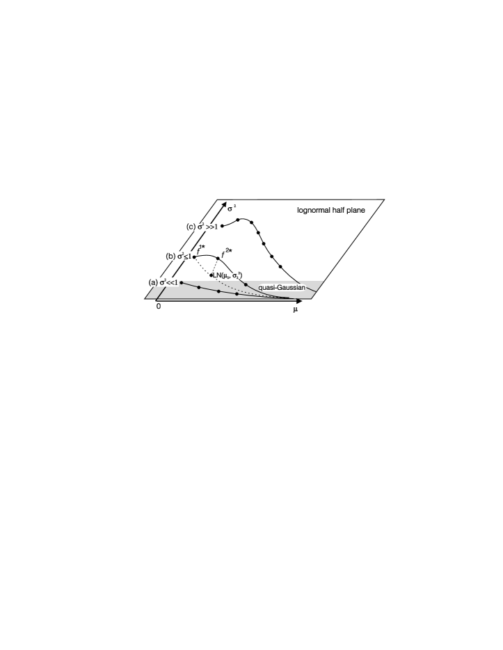
Figure 4: Schematic representation of the trajectory of $f^{n*}$ in the space of distributions. The set of lognormal distributions corresponds to the open half-plane $\left(\mu\in\mathbb{R},\sigma^{2}>0\right)$. The infinite dimension space of probability distributions is schematically represented here in three dimensions. In the region $\left(\mu\in\mathbb{R},\sigma^{2}\ll 1\right)$ (shaded area), lognormal distributions are quasi-Gaussian. (a) Narrow lognormal distributions $f^{1*}(\sigma^{2}\ll 1)$ are quasi-Gaussian and, thus, the trajectory of $f^{n*}$ starts and ends up in the close vicinity of the line $\left(\mu\in\mathbb{R},\sigma^{2}=0\right)$. (b) For moderately broad lognormal distributions ($\sigma^{2}\lesssim 1$), the trajectory of $f^{n*}$ starts in the lognormal half-plane, not too far away from the quasi-Gaussian region, that is reached for asymptotically large $n$. Thus $f^{n*}$ is conjectured to lie, for any $n$, close to the lognormal half-plane: $f^{n*}\simeq\mathrm{LN}(\mu_{n},\sigma_{n}^{2})$. (c) Very broad lognormal distributions $f^{1*}(\sigma^{2}\gg 1)$ lie far away from the quasi-Gaussian region. Thus, there is a long way before $f^{n*}$ enters the quasi-Gaussian region and $f^{n*}$ has the possibility to come significantly out of the lognormal half-plane for intermediate values of $n$.

The set of lognormal distributions can be represented by an open half-plane ($\mu$, $\sigma^{2}$) with $\mu\in(-\infty;\infty)$ and $\sigma^{2}\in(0;\infty)$. In this half-plane, the shaded region with $\sigma^{2}\ll 1$ corresponds to quasi-Gaussian lognormal distributions (see Appendix A). The whole lognormal half-plane is embedded in the infinite dimension space of probability distributions, which is schematically represented in figure 4 as a three dimension space.

The starting point $f^{1*}$ and the asymptotic behaviour $f^{n*}$ with $n\to\infty$ of the $f^{n*}$ trajectory are trivially known for any $\sigma^{2}$. Indeed, $f^{1*}=f=\mathrm{LN}(\mu,\sigma^{2})$ lies exactly in the lognormal half-plane. Moreover, the finiteness of the moments of the lognormal distribution $f^{1*}=f$ implies the applicability of the central limit theorem:

$$f^{n*}(S_{n})\mathrel{\mathop{\kern 0.0pt\to}\limits_{n\to\infty}}N\left(n\langle x\rangle,n\sigma^{2}\right)(S_{n}),$$ (29)

where $N\left(n\langle x\rangle,n\sigma^{2}\right)(S_{n})$ is narrow since its coefficient of variation $\sqrt{n\sigma^{2}}/n\langle x\rangle\propto 1/\sqrt{n}$ tends to zero. As narrow Gaussian distributions are quasi-lognormal, as shown in Appendix A, $f^{n*}$ lies close to the quasi-Gaussian region of the lognormal half-plane.

For intermediate $n$, on the contrary, the trajectory of $f^{n*}$ strongly depends on the broadness of the initial lognormal distribution $f^{1*}$ and three different cases can be distinguished.

For narrow lognormal distributions ($\sigma^{2}\ll 1$), both the starting point $f^{1*}$ and the end point $f^{n*}$ for $n=\infty$ belong to the quasi-Gaussian region. Therefore one can assume that $f^{n*}$ is quasi-Gaussian for any $n$, which gives immediately the typical sums $S_{n}^{\mathrm{t}}$ (see Section V.1).

For moderately broad lognormal distributions ($\sigma^{2}\lesssim 1$), $f^{n*}$ does not start too far away from the quasi-Gaussian region that is reached at large $n$. Hence, one can assume that $f^{n*}$ remains close to the lognormal half-plane in between $n=1$ and $n=\infty$. Thus, the approximation strategy will consist in finding a lognormal distribution $\mathrm{LN}(\mu_{n},\sigma_{n}^{2})$ (see broken line in figure 4) that closely approximates $f^{n*}$ (see Section V.2).

For very broad lognormal distributions $(\sigma^{2}\gg 1)$, $f^{n*}$ starts far away from the quasi-Gaussian region that is reached at large $n$. Hence, $f^{n*}$ may significantly come out of the lognormal half-plane. In this case, the approximation strategy is dictated by the fact that sums $S_{n}$ are dominated by the largest terms (see Section V.3).

V Derivation of the typical sums of lognormal random variables

In this section we apply the strategies discussed above in order to derive approximate analytical expressions of $S_{n}^{\mathrm{t}}$ for different ranges of $\sigma^{2}$.

V.1 Case of narrow lognormal distributions

We consider here the case $\sigma^{2}\ll 1$ of narrow lognormal distributions. As seen in Appendix A, a narrow lognormal distribution is well approximated by a normal distribution:

$$\sigma^{2}\ll 1:\mathrm{LN}\left(\mu,\sigma^{2}\right)\simeq N\left(e^{\mu},\left(\sigma e^{\mu}\right)^{2}\right)$$

Consequently, the typical sum $S_{n}^{\mathrm{t}}$ is simply given by:

$$\sigma^{2}\ll 1:S_{n}^{\mathrm{t}}\simeq ne^{\mu}$$ (30)

as in the Gaussian case, for any number of terms. Note that the law of large numbers asymptotics $S_{n}^{\mathrm{t}}\mathrel{\mathop{\kern 0.0pt\to}\limits}n\langle x\rangle=ne^{\mu+\sigma^{2}/2}$, close to eq. (30) for $\sigma^{2}\ll 1$, is applicable here even for a small number of terms.

V.2 Case of moderately broad lognormal distributions

We consider here the case $\sigma^{2}\lesssim 1$ of moderately broad lognormal distributions that already allows considerable deviation from the Gaussian behaviour obtained for $\sigma^{2}\ll 1$ (see Section V.1). The distribution $f^{n*}$ of $S_{n}$ is now conjectured to be close to a lognormal distribution:

$$\sigma^{2}\lesssim 1:f^{n*}\left(S_{n}\right)\simeq\mathrm{LN}\left(\mu_{n},\sigma_{n}^{2}\right)\left(S_{n}\right)$$ (31)

Two equations characterizing $f^{n*}$ are needed to determine the two unknown parameters $\mu_{n}$ and $\sigma_{n}^{2}$.

The cumulants provide such exact relationships on $f^{n*}$. In particular, the first two cumulants, $\langle S_{n}\rangle$ and ${\mathrm{var}}\left(S_{n}\right)$ obey:

$$\langle S_{n}\rangle=n\langle x\rangle$$ (32a)

$${\mathrm{var}}\left(S_{n}\right)=n{\mathrm{var}}\left(x\right).$$ (32b)

These equations imply

$$C_{n}^{2}=\frac{C^{2}}{n},$$ (33)

where $C_{n}\equiv\left[{\mathrm{var}}\left(S_{n}\right)\right]^{1/2}/\langle S_{n}\rangle$ is the coefficient of variation of $S_{n}$. As $f$ is lognormal and $f^{n*}$ is approximately lognormal, one has $C^{2}=e^{\sigma^{2}}-1$ and $C_{n}^{2}=e^{\sigma_{n}^{2}}-1$ (see eq. (13)). Then, using eq. (33), we obtain

$$\sigma_{n}^{2}=\ln\left(1+\frac{e^{\sigma^{2}}-1}{n}\right)=\ln\left(1+\frac{C^{2}}{n}\right).$$ (34)

At last, we derive $\mu_{n}$ by developing eq. (32a) using eq. (11):

$$e^{\mu_{n}+\sigma_{n}^{2}/2}=ne^{\mu+\sigma^{2}/2}.$$ (35)

Thus, thanks to eq. (34), one has:

$$\mu_{n} = \mu+\frac{\sigma^{2}}{2}+\ln\left(\frac{n}{\sqrt{1+\frac{e^{\sigma^{2}}-1}{n}}}\right)$$ (36)

$$= \ln\left(n\langle x\rangle\right)-\frac{1}{2}\ln\left(1+\frac{C^{2}}{n}\right)$$

In the remainder of this section, we will examine the consequences of eq. (34) and eq. (36) on the typical sum $S_{n}^{\mathrm{t}}$, on the height of the peak of $f^{n*}$ and on the convergence of $f^{n*}$ to a Gaussian.

The typical sum $S_{n}^{\mathrm{t}}$ derives from eq. (34), eq. (36) and eq. (9):

$$\sigma^{2}\lesssim 1:\quad S_{n}^{\mathrm{t}}\simeq n\langle x\rangle\frac{1}{\left(1+\frac{C^{2}}{n}\right)^{3/2}}.$$ (37)

The typical sum $S_{n}^{\mathrm{t}}$ appears as the product of the usual law of large numbers, $n\langle x\rangle$, and of a ’correction’ factor, $(1+C^{2}/n)^{-3/2}$, which can be very large. The square of the coefficient of variation defines a scale for $n$: when $n\gg C^{2}$, the law of large numbers approximately holds, whereas when $n\ll C^{2}$, the law of large numbers grossly overestimates $S_{n}^{\mathrm{t}}$. If the initial lognormal distributions is broader, $C^{2}$ is larger and, thus, larger $n$’s are required for the law of large numbers to apply. We analyze now more precisely the small $n$ and large $n$ behaviours.

For $n=1$, eq. (37) gives $S_{1}^{\mathrm{t}}\simeq e^{\mu-\sigma^{2}}$ which is, as it should be, the exact expression for the typical value $x^{\mathrm{t}}$ of a single lognormal term (see eq. (9)). For small $n$, we obtain

$$n\ll C^{2}:\quad S_{n}^{\mathrm{t}}\simeq n^{5/2}\frac{\langle x\rangle}{C^{3}},$$ (38)

i.e., a much faster dependence on $n$ then in the usual law of large numbers; this evokes a Lévy flight with exponent $\alpha=2/5$ (see eq. (24)). For large $n$, the expression eq. (37) expands into :

$$n\gg C^{2}:\quad S_{n}^{\mathrm{t}}\simeq n\langle x\rangle-\frac{3}{2}C^{2}\langle x\rangle.$$ (39)

The practical consequences of these expressions appear clearly on the sample mean $Y_{n}$:

$$Y_{n}\equiv\frac{S_{n}}{n}.$$ (40)

Eq. (38) and eq. (39) give the typical sample mean $Y_{n}^{\mathrm{t}}$:

$$n\ll C^{2}:\quad Y_{n}^{\mathrm{t}}\simeq\left(\frac{n}{C^{2}}\right)^{3/2}\langle x\rangle$$ (41a)

$$n\gg C^{2}:\quad Y_{n}^{\mathrm{t}}\simeq\langle x\rangle-\frac{3}{2}\frac{C^{2}}{n}\langle x\rangle.$$ (41b)

Thus, for small systems $\left(n\ll C^{2}\right)$, one has $Y_{n}^{\mathrm{t}}\ll\langle x\rangle$. In other words, the sample mean of a small system does not typically yield the average value. For instance, if $\sigma^{2}=4$, $Y_{1}^{\mathrm{t}}\simeq\langle x\rangle/400$. This is important, e.g., for tunnel junctions Costa et al. (2002) and contradicts common implicit assumptions Chow (1963); Hurych (1966). For large systems ($n\gg C^{2}$), one recovers the average value. However, the correction to the average value decreases slowly with $n$, as $1/n$, and might be measurable even for a relatively large $n$. Thus, macroscopic measurements may give access to microscopic fluctuations, which is important for physics applications. Usually, microscopic fluctuations average out so that they can not easily be extracted from macroscopic measurements. This property, often taken for granted, comes from the fast convergence of sums $S_{n}$ to the law of large numbers asymptotics, which only occurs with narrow distributions.

We consider now the peak height $g_{n}(Y_{n}^{\mathrm{t}})$ of the distribution

$$g_{n}(Y_{n})\equiv nf^{n*}(S_{n})$$ (42)

of the sample mean $Y_{n}$ (figure 5).

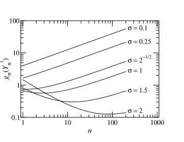
Figure 5: Peak height $g_{n}(Y_{n}^{\mathrm{t}})$ of the distribution of the sample mean $Y_{n}=S_{n}/n$. Initial lognormal distribution: $\mathrm{LN}(\mu=0,\sigma^{2})$. For narrow lognormal distributions ($\sigma^{2}<1/2$), $g_{n}(Y_{n}^{\mathrm{t}})$ always increases with $n$ (normal behaviour). For broader lognormal distributions ($\sigma^{2}>1/2$), $g_{n}(Y_{n}^{\mathrm{t}})$ presents an unusual decrease with $n$ at small $n$ indicating that the peak of $g_{n}(Y_{n})$ broadens, even if its far tail becomes lighter as usual.

Combining eq. (15) and eq. (31) via eq. (34) and eq. (36) gives:

$$g_{n}(Y_{n}^{\mathrm{t}})=\frac{1+C^{2}/n}{\sqrt{2\pi}\langle x\rangle\sqrt{\ln(1+C^{2}/n)}}.$$ (43)

A simple study, for the non trivial case $\sigma^{2}>1/2$, reveals that $g_{n}(Y_{n}^{\mathrm{t}})$ decreases from $n=1$ to $n=C^{2}/(e^{1/2}-1)$ $(>1)$ and then increases for larger values of $n$. This echoes the non-monotonous dependence on $\sigma^{2}$ of the peak height of a lognormal distribution $f$ (see eq. (15) and related comments). The increase at large $n$ simply corresponds to the narrowing of the distribution of $Y_{n}=S_{n}/n$ when $n$ increases, as predicted by the law of large numbers. Moreover, the large $n$ expansion of eq. (43) gives $g_{n}(Y_{n}^{\mathrm{t}})\simeq\frac{\sqrt{n}}{\sqrt{2\pi{\mathrm{var}}\left(x\right)}}$, which is the prediction of the central limit theorem, as it should be. On the other hand, the decrease of $g_{n}(Y_{n}^{\mathrm{t}})$ at small $n$ is less usual. The peak of $g_{n}(Y_{n})$ is actually broader than the one of the unconvoluted distribution $g_{1}=f$. This behaviour can be understood in the following way. If the lognormal distribution $f(x)$ is broad enough ($C^{2}\gg 1$), it presents at the same time a high and narrow peak at small $x$ and a long tail at large $x$. The effect of convoluting $f$ with itself is first ($n<C^{2}/(e^{1/2}-1)$) to ‘contaminate’ the peak with the (heavy) tail. This results in a broadening and decrease of the $f^{n*}(S_{n})$ peak which is strong enough to entail a decrease of the $g_{n}(Y_{n})=nf^{n*}(S_{n})$ peak. On the contrary, when enough convolutions have taken place ($n>C^{2}/(e^{1/2}-1)$), the shape parameter $\sigma_{n}^{2}$ (eq. (34)) becomes small and the tail of $f^{n*}$ becomes light. Under these circumstances, further convolution mainly ‘mixes’ the peak with itself. This results in a broadening and decrease of the $f^{n*}(S_{n})$ peak which is weak enough to allow an increase of the $g_{n}(Y_{n})=nf^{n*}(S_{n})$ peak.

The small $n$ decrease of $g_{n}(Y_{n})$ has physical consequences. There is a range of sample sizes, corresponding to $n<C^{2}/(e^{1/2}-1)$ for which the precise determination of the typical values becomes more difficult when the sample size increases. This is a striking effect of the broad character of the lognormal distribution. On the contrary, for narrow distributions, the determination of the typical value becomes more accurate as the sample size increases.

At last, we examine the compatibility of the obtained $f^{n*}$ with the central limit theorem by studying the distribution $h_{n}(Z_{n})=f^{n*}(S_{n}){\mathrm{d}}S_{n}/{\mathrm{d}}Z_{n}$ of the usual rescaled random variable $Z_{n}$:

$$Z_{n}\equiv\frac{S_{n}-n\langle x\rangle}{\sqrt{n~{}{\mathrm{var}}\left(x\right)}}.$$ (44)

Simple derivations using eq. (13) and eq. (11) lead to

$$h_{n}(Z_{n})\simeq\frac{C}{\sqrt{2\pi n\ln\left(1+\frac{C^{2}}{n}\right)}\left(1+\frac{CZ_{n}}{\sqrt{n}}\right)}$$

$$\exp\left\{\frac{-\left[\ln\left(1+\frac{CZ_{n}}{\sqrt{n}}\right)+\frac{1}{2}\ln\left(1+\frac{C^{2}}{n}\right)\right]^{2}}{2\ln\left(1+\frac{C^{2}}{n}\right)}\right\}.$$ (45)

For $n\gg C^{2}$ and $|CZ_{n}/\sqrt{n}|\ll 1$, one has $\ln(1+C^{2}/n)\simeq C^{2}/n$ and $\ln(1+CZ_{n}/\sqrt{n})\simeq CZ_{n}/\sqrt{n}-(CZ_{n})^{2}/2n$, which gives:

$$h_{n}(Z_{n})\simeq\frac{1}{\sqrt{2\pi}\left(1+\frac{CZ_{n}}{\sqrt{n}}\right)}\;\exp\left\{\frac{-\left[Z_{n}+\frac{C}{2\sqrt{n}}\left(1-Z_{n}^{2}\right)\right]^{2}}{2}\right\}.$$ (46)

Clearly, the central limit theorem is recovered:

$$h_{n}(Z_{n})\to\frac{1}{\sqrt{2\pi}}e^{-Z_{n}^{2}/2}\quad\mathrm{when}\quad n\to\infty,$$ (47)

consistently with the strategy defined in Section IV (see eq. (29)). Moreover, the square of the coefficient of variation appears in eq. (46) as the convergence scale of $f^{n*}$ to the central limit theorem. As shown in eq. (37), $C^{2}$ is also the convergence scale of $S_{n}^{\mathrm{t}}$ to the law of large numbers.

V.3 Case of very broad lognormal distributions

We consider here the case $\sigma^{2}\gg 1$ of very broad lognormal distributions. To treat this complex case, we will proceed through different steps, in a more heuristic way than in the previous cases.

The first step is to assume that the sums $S_{n}$ are typically dominated by the largest term $M_{n}$, if $n$ is not too large (see eq. (20) and Section III) . Thus, the distribution function of $S_{n}$, defined as the probability that $S_{n}<x$ and denoted as ${\mathrm{Pr}}\left({S_{n}}<{x}\right)$, is approximately equal to the distribution function of $M_{n}$, denoted as ${\mathrm{Pr}}\left({M_{n}}<{x}\right)$:

$$\sigma^{2}\gg 1:{\mathrm{Pr}}\left({S_{n}}<{x}\right)\simeq{\mathrm{Pr}}\left({M_{n}}<{x}\right).$$ (48)

As $M_{n}$ is the largest term of all $x_{i}$’s, $M_{n}<x$ is equivalent to $x_{i}<x$ for all $i=1,\ldots,n$. Thus,

$${\mathrm{Pr}}\left({M_{n}}<{x}\right)={\mathrm{Pr}}\left({x_{1}}<{x}\right)\times\cdots\times{\mathrm{Pr}}\left({x_{n}}<{x}\right)=\left[{\mathrm{F}}\left(x\right)\right]^{n}$$ (49)

where ${\mathrm{F}}\left(x\right)\equiv\int_{0}^{x}{f(x^{\prime}){\mathrm{d}}x^{\prime}}$ is the distribution function of the initial lognormal distribution. This implies

$${\mathrm{Pr}}\left({S_{n}}<{x}\right)\simeq\left[{\mathrm{F}}\left(x\right)\right]^{n}$$ (50)

. By definition, the typical sum $S_{n}^{\mathrm{t}}$ is given by ${\mathrm{d}}^{2}{{\mathrm{Pr}}\left({S_{n}}<{x}\right)}/{\mathrm{d}}{x^{2}}=0$, which, from eq. (50), leads to:

$$-\left(\sigma+y_{n}\right)\sqrt{2\pi}\Phi\left(y_{n}\right)+\left(n-1\right)e^{-y_{n}^{2}/2}=0$$ (51)

where $y_{n}\equiv\left(\ln S_{n}^{\mathrm{t}}-\mu\right)/\sigma$ and $\Phi\left(y\right)\equiv\left(2\pi\right)^{-1/2}\int_{-\infty}^{y}{e^{-u^{2}/2}{\mathrm{d}}u}$ is the distribution function of the standard normal distribution $\mathrm{N}\left(0,1\right)$. This equation has no exact explicit solution. However, as $y_{1}=-\sigma\ll-1$ (use eq. (9) with $S_{1}^{\mathrm{t}}=x^{\mathrm{t}}$), let us assume that $y_{n}\ll-1$ also for $n>1$. Then we can approximate $\Phi\left(y_{n}\right)$ by $\Phi\left(y_{n}\right)\simeq-e^{-y_{n}^{2}/2}/\sqrt{2\pi}y_{n}$ (see, e.g., Abramowitz and Stegun (1972), chap. 26). This leads to a linear equation on $y_{n}$, giving $y_{n}\simeq-\sigma/n$, valid for $y_{n}\ll-1$, i.e., $n<\sigma$. Finally, one has:

$$\sigma^{2}\gg 1,n<\sigma:S_{n}^{\mathrm{t}}\simeq e^{\mu-\sigma^{2}/n}.$$ (52)

For $n=1$ this expression is exact. When $n$ increases till $n=\sigma^{2}$, eq. (52) gives an unusually fast, exponential dependence on $n$ that is in contrast with, e.g., the $n^{5/2}$ dependence obtained for $\sigma^{2}\lesssim 1$ and $n\ll C^{2}$ (eq. (38)). Unfortunately, when $n$ becomes larger, eq. (52) is qualitatively wrong. Indeed, it implies $S_{n}^{\mathrm{t}}/n\to e^{\mu}/n\to 0$ instead of $S_{n}^{\mathrm{t}}/n\to\langle x\rangle$ as predicted by the law of large numbers.

The second step, improving eq. (52), consists in combining eq. (52) with a cumulant constraint. We assume that $f^{n*}\simeq\mathrm{LN}\left(\mu_{n},\sigma_{n}^{2}\right)$ as in Section V.2 for all $n=2^{j}$, with $j=1,2,\ldots$ and that the typical sum $S_{2^{j+1}}^{\mathrm{t}}$ is $e^{\mu_{2^{j}}-\sigma_{2^{j}}^{2}/2}$ as in eq. (52) since $S_{2^{j}}$ is considered as lognormal. We use these assumptions and $\langle S_{2^{j+1}}\rangle=2^{j+1}\langle x\rangle$ to determine induction relations between $\left(\mu_{2^{j+1}},\sigma_{2^{j+1}}^{2}\right)$ and $\left(\mu_{2^{j}},\sigma_{2^{j}}^{2}\right)$, which leads to:

$$\sigma_{2^{j}}^{2}=\left(\frac{2}{3}\right)^{j}\sigma^{2}+2\left[1-\left(\frac{2}{3}\right)\right]\ln 2,$$ (53a)

$$\mu_{2^{j}}=\mu+\left(\frac{\sigma^{2}}{2}-\ln 2\right)\left[1-\left(\frac{2}{3}\right)^{j}\right]+j\ln 2.$$ (53b)

The typical sum is then

$$S_{n}^{\mathrm{t}}\simeq n\langle x\rangle\exp\left[-\frac{3}{2}\frac{\sigma^{2}}{n^{\ln\left(3/2\right)/\ln 2}}-3\ln 2\left(1-\frac{1}{n^{\ln\left(3/2\right)/\ln 2}}\right)\right].$$ (54)

Eq. (54) is still exact for $n=1$ and it clearly improves on eq. (52) for large $n$. Indeed, when $n\to\infty$, $S_{n}^{\mathrm{t}}/n$ no longer tends to 0. However, $S_{n}^{\mathrm{t}}/n$ tends to $\langle x\rangle/8$ instead of $\langle x\rangle$, which is the signature of a leftover problem. This comes from the assumptions that $f^{n*}\simeq\mathrm{LN}\left(\mu_{n},\sigma_{n}^{2}\right)$, which may be correct for large $n$ (small $\sigma_{n}^{2}$) but is excessive for small $n$ (large $\sigma_{n}^{2}$), and that $S_{2^{j+1}}^{\mathrm{t}}\simeq e^{\mu_{2^{j}}-\sigma_{2^{j}}^{2}/2}$, which is correct for small $n=2^{j}$ (large $\sigma_{n}^{2}$) but is excessive for large $n$ (small $\sigma_{n}$).

The third step, in order to cure the main problem of eq. (54), is to wildly get rid of the last term in the exponential which prevents $S_{n}^{\mathrm{t}}$ from converging to $n\langle x\rangle$ at large $n$, which does not affect the validity for $n=1$:

$$\sigma^{2}\gg 1:\quad S_{n}^{\mathrm{t}}\simeq n\langle x\rangle\exp\left[-\frac{3}{2}\frac{\sigma^{2}}{n^{\ln\left(3/2\right)/\ln 2}}\right].$$ (55)

We have tried to empirically improve this formula by looking for a better exponent $\alpha$ than $\ln\left(3/2\right)/\ln 2$ for $\sigma^{2}\in\left[0.25,16\right]$. Unfortunately, no single $\alpha$ value is adequate for all $\sigma$’s. Eq. (55) with $\alpha=\ln\left(3/2\right)/\ln 2$ stands up as a good compromise for the investigated $\sigma$-range.

VI Range of validity of formulae

In this section we proceed to the numerical determination of the range of validity of the three theoretical formulae given by eq. (30), eq. (37) and eq. (55) for the typical sum of $n$ lognormal terms.

In order to fulfil this task, the typical sample mean $Y_{n}^{\mathrm{t}}$ (eq. (40)) instead of $S_{n}^{\mathrm{t}}$ will be used. This has the advantage of showing only the discrepancies to the mean value without the obvious proportionality of $S_{n}^{\mathrm{t}}$ on $n$ resulting from the law of large numbers. The values of $Y_{n}^{\mathrm{t}}$ computed using the three theoretical formulae eq. (30), eq. (37) and eq. (55) are called $Y_{n,\mathrm{I}}^{\mathrm{t}}$, $Y_{n,\mathrm{II}}^{\mathrm{t}}$ and $Y_{n,\mathrm{III}}^{\mathrm{t}}$ respectively:

$$\sigma^{2}\ll 1:\quad Y_{n,\mathrm{I}}^{\mathrm{t}}=e^{\mu},$$ (56a)

$$\sigma^{2}\lesssim 1:\quad Y_{n,\mathrm{II}}^{\mathrm{t}}=\langle x\rangle\left(1+\frac{C^{2}}{n}\right)^{-3/2},$$ (56b)

$$\sigma^{2}\gg 1:\quad Y_{n,\mathrm{III}}^{\mathrm{t}}=\langle x\rangle\exp\left[-\frac{3}{2}\,\frac{\sigma^{2}}{n^{\ln(3/2)/\ln 2}}\right].$$ (56c)

The exact typical sample mean, derived from Monte Carlo generation of the distributions $g_{n}(Y_{n})$, is called $Y_{n,\mathrm{ex}}^{\mathrm{t}}$. Enough Monte-Carlo draws ensure negligible statistical uncertainty. As an example, we show in figure 6 the obtained distributions $g_{n}(Y_{n})$ for $\mu=0$ and $\sigma=1.5$.

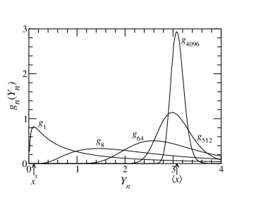
Figure 6: Distributions $g_{n}(Y_{n})$ of the sample mean $Y_{n}$ for an initial lognormal with $\mu=0$ and $\sigma=1.5$.

Notice that $Y_{n,\mathrm{ex}}^{\mathrm{t}}$ moves from $Y_{1,\mathrm{ex}}^{\mathrm{t}}=x^{\mathrm{t}}=e^{-\sigma^{2}}\simeq 0.11$ to $Y_{\infty,\mathrm{ex}}^{\mathrm{t}}=\langle x\rangle=e^{\sigma^{2}/2}\simeq 3.08$. To determine the $Y_{n,\mathrm{ex}}^{\mathrm{t}}$’s, shown as solid line in figure 7, the absolute maximum of $g_{n}(Y_{n})$ is obtained by parabolic least square fits performed on the $\log/\log$ representation of each distribution. Moreover, in the latter figure, we also show $Y_{n,\mathrm{I}}^{\mathrm{t}}$ (dots), $Y_{n,\mathrm{II}}^{\mathrm{t}}$ (circles) and $Y_{n,\mathrm{III}}^{\mathrm{t}}$ (squares).

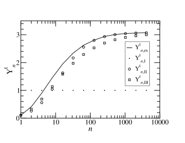
Figure 7: $Y_{n,\mathrm{ex}}^{\mathrm{t}}$ (solid line) for an initial $\sigma=1.5\ \left(\mu=0\right)$ as well as $Y_{n,\mathrm{I}}^{\mathrm{t}}$ ($\sigma^{2}\ll 1$, dots), $Y_{n,\mathrm{II}}^{\mathrm{t}}$ ($\sigma^{2}\lesssim 1$, circles) and $Y_{n,\mathrm{III}}^{\mathrm{t}}$ ($\sigma^{2}\gg 1$, squares).

To determine the validity range of the theoretical formulae, we define two error estimators. The first one is the maximum relative error $\delta_{\mathrm{rel,(I,\ II,\ or\ III)}}$, i.e.,   the maximum deviation referred to the minimum between $Y_{n,\mathrm{(I,\ II,\ or\ III)}}^{\mathrm{t}}$ and $Y_{n,\mathrm{ex}}^{\mathrm{t}}$, which is defined as follows:

$$\delta_{\mathrm{rel,}i}\equiv\max\left(\frac{Y_{n,i}^{\mathrm{t}}-Y_{n,\mathrm{ex}}^{\mathrm{t}}}{Y_{n,\mathrm{ex}}^{\mathrm{t}}},\frac{Y_{n,\mathrm{ex}}^{\mathrm{t}}-Y_{n,i}^{\mathrm{t}}}{Y_{n,i}^{\mathrm{t}}};n=1,2,\ldots\right)$$ (57)

and can be transformed into:

$$\delta_{\mathrm{rel,}i}=\max\left[e^{\left|\ln\left(\frac{Y_{n,i}^{\mathrm{t}}}{Y_{n,\mathrm{ex}}^{\mathrm{t}}}\right)\right|}-1;n=1,2,\ldots\right].$$ (58)

The second one is the maximum scale error $\delta_{\mathrm{scale,(I,II\ or\ III)}}$, i.e.,  the maximum deviation in magnitude referred to the total amplitude of the phenomenon:

$$\delta_{\mathrm{scale},i}\equiv\max\left[\left|\frac{\ln\left(Y_{n,i}^{\mathrm{t}}/Y_{n,\mathrm{ex}}^{\mathrm{t}}\right)}{\ln\left(Y_{\infty,\mathrm{ex}}^{\mathrm{t}}/Y_{1,\mathrm{ex}}^{\mathrm{t}}\right)}\right|;n=1,2,\ldots\right].$$ (59)

Using eq. (9) for $Y_{1,\mathrm{ex}}^{\mathrm{t}}$ and eq. (17) for $Y_{\infty,\mathrm{ex}}^{\mathrm{t}}$, $\delta_{\mathrm{scale},i}$ boils down to:

$$\delta_{\mathrm{scale},i}=\max\left[\left|\frac{2\ln\left(Y_{n,i}^{\mathrm{t}}/Y_{n,\mathrm{ex}}^{\mathrm{t}}\right)}{3\sigma^{2}}\right|;n=1,2,\ldots\right].$$ (60)

Remark that $\delta_{\mathrm{rel},i}=\exp\left(\frac{3\sigma^{2}}{2}\delta_{\mathrm{scale},i}\right)-1$. The first step for computing $\delta_{\mathrm{rel},i}$ and $\delta_{\mathrm{scale},i}$ is thus to find the value of $n$ for which $\left|\ln\left(Y_{n,i}^{\mathrm{t}}/Y_{n,\mathrm{ex}}^{\mathrm{t}}\right)\right|$ is maximum. For the data shown in figure 7, we find $n=1$ for eq. (56a), $n=4$ for eq. (56b) and $n=4$ for eq. (56c), which gives $\delta_{\mathrm{rel,I}}=849\%$ ($\delta_{\mathrm{scale,I}}=67\%$), $\delta_{\mathrm{rel,II}}=61\%$ ($\delta_{\mathrm{scale,II}}=14\%$) and $\delta_{\mathrm{rel,III}}=31\%$ ($\delta_{\mathrm{scale,III}}=8\%$).

To work out the dependences of $\delta_{\mathrm{rel},i}$ (figure 8) and $\delta_{\mathrm{scale},i}$ (figure 9) as functions of $\sigma$, the same kind of calculation is performed for $\sigma\in(0,4]$ which is the relevant range for the chosen physics applications.

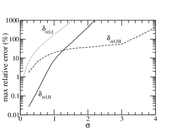
Figure 8: Maximum relative errors $\delta_{\mathrm{rel},i}$ as functions of $\sigma$.

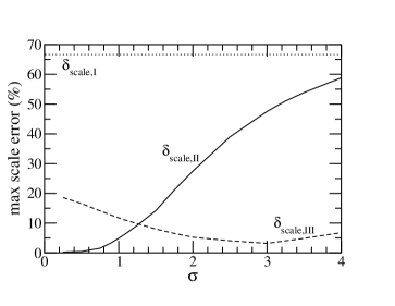
Figure 9: Maximum scale errors $\delta_{\mathrm{scale},i}$ as function of $\sigma$.

The dotted lines representing $\delta_{\mathrm{rel,I}}$ and $\delta_{\mathrm{scale,I}}$ show that the first theoretical formula is the least accurate in the explored $\sigma$ range. However, for its domain of application, $\sigma^{2}\ll 1$, the error is acceptable for $\delta_{\mathrm{rel,I}}$ ($\delta_{\mathrm{rel,I}}\simeq\sigma^{2}$, see ). Indeed, $\delta_{\mathrm{rel,I}}\lesssim 7\%$ for $\sigma\in[0,0.25]$ which, in turn, means that lognormal distributions are quasi-Gaussian in this range (see shaded area in figure 4). The solid lines representing $\delta_{\mathrm{rel,II}}$ and $\delta_{\mathrm{scale,II}}$ show that the second theoretical formula is the most accurate in the range $0\leq\sigma\lesssim 1.25$ giving $\delta_{\mathrm{rel,II}}\lesssim 30\%$ and $\delta_{\mathrm{scale,II}}\lesssim 10\%$. Note that good tunnel junctions fall within this $\sigma$ range. The broken lines representing $\delta_{\mathrm{rel,III}}$ and $\delta_{\mathrm{scale,III}}$ show that the third theoretical formula is the most accurate for $\sigma\gtrsim 1.25$ and is reasonably accurate for $\sigma\lesssim 1.25$. Note that, for $\sigma=4$, the maximum relative error $\delta_{\mathrm{rel,III}}\simeq 400\%$ appears quite high. However, when the error is referred to the total amplitude of the scaling, as given by $\delta_{\mathrm{scale,III}}$, it is only $7\%$.

Importantly, the observed ranges of validity of the three different formulae are consistent with the strategies of approximation used to derive these formulae. This provides an a posteriori confimation of the theoretical analysis presented in the paper.

VII A striking effect: scaling of the sample mean and of its inverse

In general, if a function is increasing, its inverse is decreasing. What happens if one considers the typical values of a random variable and of its inverse ? Does one have :

$$z_{n}^{t}\nearrow\iff\left(1/z_{n}\right)^{t}\searrow\quad?$$ (61)

While this is intuitively true for narrow distributions, it may fail for broad distributions.

This problem arises in electronics, where it is customary to study the product $R\times A$ of the device resistance $R$ by the device size $A$. One usually checks that $R\times A$ does not depend on $A$, otherwise this dependence is taken as the indication of edge effects. The resistance $R$ being the inverse of the conductance can be represented by $1/S_{n}$ where $S_{n}$ is the sum of $n$ independent conductances. The size $A$ of the system is proportional to $n$. Hence, one has:

$$R\times A\propto\frac{n}{S_{n}}=\frac{1}{Y_{n}},$$ (62)

where $Y_{n}$ is the sample mean of conductances. We have shown that the typical $Y_{n}$ increases with the sample size (see eqs. (56)), if conductances are lognormally distributed. Hence, $R\times A$ being proportional to the inverse of $Y_{n}$, one naively expects a decrease of the typical value of $R\times A$ with $n\propto A$.

What do the results presented in this paper imply for the typical value of $R\times A$? Let us do the correct calculation in the case $\sigma^{2}\lesssim 1$, relevant for good tunnel junctions. As $f^{n*}\left(S_{n}\right)\simeq\mathrm{LN}\left(\mu_{n},\sigma_{n}^{2}\right)\left(S_{n}\right)$, the distribution of $1/Y_{n}$ is:

$$\mathrm{LN}\left(-\mu_{n}+\ln n,\sigma_{n}^{2}\right)\left(1/Y_{n}\right)$$ (63)

(see Section II). The typical sample mean inverse is thus, using eqs. (34) and (36):

$$\sigma^{2}\lesssim 1:\quad\left(1/Y_{n}\right)^{\mathrm{t}}\simeq\frac{1}{\langle x\rangle\left(1+\frac{C^{2}}{n}\right)^{1/2}}.$$ (64)

Thus just as $Y_{n}^{\mathrm{t}}$, $\left(1/Y_{n}\right)^{\mathrm{t}}$ increases with the sample size!

This counterintuitive result epitomizes the paradoxical behaviour of some broad distributions. Moreover, this can be a possible explanation for the anomalous scaling of $R\times A$ observed for small magnetic tunnel junctions Lee et al. (2002).

VIII Conclusion

We have studied the typical sums of $n$ lognormal random variables. Approximate formulae have been obtained for three different regimes of the shape parameter $\sigma^{2}$. Table 1 summarizes these results with their ranges of applicability.

Table 1: Range of applicability of the different formulae. Errors are measured by $\delta_{\mathrm{rel}}$ and $\delta_{\mathrm{scale}}$, see Section VI for details.

$S_{n}^{\mathrm{t}}$	$\sigma$ range	$\delta_{\mathrm{rel}}$	$\delta_{\mathrm{scale}}$
$ne^{\mu}$	$\left[0,0.25\right]$	$\leq 7\%$	$\leq 67\%$
$n\langle x\rangle\frac{1}{\left(1+\frac{C^{2}}{n}\right)^{3/2}}$	$\left[0,1.25\right]$	$\leq 30\%$	$\leq 10\%$
$n\langle x\rangle\exp\left[-\frac{3}{2}\frac{\sigma^{2}}{n^{\ln\left(3/2\right)/\ln 2}}\right]$	$\left[1.25,4\right]$	$\leq 400\%$	$\leq 7\%$

These results are relevant up to $\sigma\lesssim 4$; for larger $\sigma$, one may apply the theorems in Arous et al. (2002) and Bovier et al. (2002).

The anomalous behaviour of the typical sums has been related to the broadness of lognormal distributions. For large enough shape parameter $\sigma^{2}$, the behaviour of lognormal sums is non trivial. It reveals properties of broad distributions at small sample sizes and properties of narrow distributions at large sample sizes with a slow transition between the two regimes. Counter-intuitive effects have been pointed out like the decrease of the peak height of the sample mean distribution with the sample size and the fact that the typical sample mean and its inverse do not vary with the sample size in opposite ways. Finally, we have shown that the statistical effects arising from the broadness of lognormal distributions have observable consequences for moderate size physical systems.

Appendix A Approximation of narrow lognormal distributions by normal distributions and vice versa

As seen in Section II, the lognormal probability distribution $f(x)=\mathrm{LN}(\mu,\sigma^{2})(x)$ is mostly concentrated in the interval $\left[e^{\mu}e^{-\sigma},e^{\mu}e^{\sigma}\right]$. If $\sigma\ll 1$, this range is small and can be rewritten as:

$$e^{\mu}\left(1-\sigma\right)\lesssim x\lesssim e^{\mu}\left(1+\sigma\right).$$ (65)

Thus it makes sense to expand $f(x)$ around its typical value $e^{\mu}$ by introducing a new random variable $\epsilon$ defined by:

$$x\equiv e^{\mu}\left(1+\epsilon\right),$$ (66)

where $\epsilon$ is a random variable on the order of $\sigma$:

$$-\sigma\lesssim\epsilon\lesssim\sigma.$$ (67)

As $\sigma\ll 1$, this entails $\left|\epsilon\right|\ll 1$. Expanding the lognormal distribution $f(x)$ of eq. (1) in powers of $\epsilon$ leads to:

$$f(x) \simeq \frac{1}{\sqrt{2\pi\sigma^{2}}e^{\mu}}\left(1-\epsilon+\epsilon^{2}+\cdots\right)$$ (68)

$$\exp\left(-\frac{\epsilon^{2}}{2\sigma^{2}}+\frac{\epsilon^{3}}{2\sigma^{2}}+\cdots\right)$$

The dominant term gives $f(x)\simeq\frac{1}{\sqrt{2\pi\sigma^{2}}e^{\mu}}\exp\left(-\frac{\epsilon^{2}}{2\sigma^{2}}\right)$, thus using eq. (66):

$$f(x)\simeq\frac{1}{\sqrt{2\pi\left(\sigma e^{\mu}\right)^{2}}}\exp\left[-\frac{\left(x-e^{\mu}\right)^{2}}{2\left(\sigma e^{\mu}\right)^{2}}\right]$$ (69)

In other words, a narrow lognormal distribution is well approximated by a normal distribution:

$$\sigma\ll 1:\mathrm{LN}\left(\mu,\sigma^{2}\right)\simeq N\left(e^{\mu},\left(\sigma e^{\mu}\right)^{2}\right)$$ (70)

More intuitively, the Gaussian approximation of narrow lognormal distributions $\mathrm{LN}\left(\mu,\sigma^{2}\right)\left(x\right)$ can be inferred from the underlying Gaussian random variable $y$ with distribution $N\left(0,1\right)\left(y\right)$, with $x=e^{\mu+\sigma y}$. Since $\left|y\right|\simeq 1$ and $\sigma\ll 1$, one has $\left|\sigma y\right|\ll 1$ and, thus, $x\simeq e^{\mu}\left(1+\sigma y\right)$. Consequently, $x$ being a linear transformation of a Gaussian random variable, is itself normally distributed according to $N\left(e^{\mu},\left(\sigma e^{\mu}\right)^{2}\right)$, in agreement with eq. (70).

Conversely, a narrow $\left(\sigma\ll\mu\right)$ Gaussian distribution $N\left(\mu,\sigma^{2}\right)$ can be approximated by a lognormal distribution:

$$\sigma\ll 1:N\left(\mu,\sigma^{2}\right)\simeq\mathrm{LN}\left(\ln\mu,\left(\sigma/\mu\right)^{2}\right).$$ (71)

For completeness, one can easily show that any Gaussian distribution $N\left(\mu,\sigma^{2}\right)$ can be approximated by a three parameter lognormal distribution $\mathrm{LN}\left(\ln\left(\mu+A\right),\left(\frac{\sigma}{\mu+A}\right)^{2},A\right)$ where $A$ is any number such that $A+\mu\gg\sigma$. The probability density of the three parameter lognormal distribution is $\mathrm{LN}\left(\mu,\sigma^{2},A\right)=\frac{1}{\sqrt{2\pi\sigma^{2}}\left(x-A\right)}\exp\left\{-\frac{\left[\ln\left(x-A\right)-\mu\right]^{2}}{2\sigma^{2}}\right\}$ for $x>A$ and $0$ otherwise.

References

- Bouchaud and Georges (1990) J.-P. Bouchaud and A. Georges, Phys. Rep. 195, 127 (1990).
- Shlesinger et al. (1995) M. F. Shlesinger, G. M. Zaslavsky, and U. Frisch, eds., Lévy Flights and Related Topics in Physics, vol. 450 of Lecture Notes in Physics (Springer-Verlag, Berlin, 1995).
- Kutner et al. (1999) R. Kutner, A. Pȩkalski, and K. Sznajd-Weron, eds., Anomalous diffusion: from basics to applications, Proceedings of the XIth Max Born Symposium Held at La̧dek Zdrój, Poland, 20-27 May 1998 (Springer-Verlag, Berlin, 1999).
- Moodera et al. (1995) J. S. Moodera, L. R. Kinder, T. M. Wong, and R. Meservey, Phys. Rev. Lett. 74, 3273 (1995).
- Miyazaki and Tezuka (1995) T. Miyazaki and N. Tezuka, J. Magn. Magn. Mater. 151, 403 (1995).
- Bardou (1997) F. Bardou, Europhys. Lett. 39, 239 (1997).
- Costa et al. (2000a) V. D. Costa, Y. Henry, F. Bardou, M. Romeo, and K. Ounadjela, Eur. Phys. J. B 13, 297 (2000a).
- Kelly (1999) M. J. Kelly, Semicond. Sci. Tech. 14, 1 (1999).
- Costa et al. (2002) V. D. Costa, M. Romeo, and F. Bardou, J. Magn. Magn. Mater. pp. to appear and cond–mat/0205473 (2002).
- Cassan et al. (1999) E. Cassan, S. Galdin, P. Dollfus, and P. Hesto, J. Appl. Phys. 86, 3804 (1999).
- Momose et al. (1998) H. S. Momose, S. Nakamura, T. Ohguro, T. Yoshitomi, E. Morifuji, T. Morimoto, Y. Katsumata, and H. Iwai, IEEE Transactions on Electron Devices 45, 691 (1998).
- Costa et al. (1998) V. D. Costa, F. Bardou, C. Béal, Y. Henry, J. P. Bucher, and K. Ounadjela, J. Appl. Phys. 83, 6703 (1998).
- Limpert et al. (2001) E. Limpert, W. A. Stahel, and M. Abbt, BioScience 51, 341 (2001).
- Bouchaud and Potters (2000) J.-P. Bouchaud and M. Potters, Theory of Financial Risks (Cambridge University Press, Cambridge, 2000).
- Crow and Shimizu (1988) E. L. Crow and K. Shimizu, eds., Lognormal distributions (Marcel Dekker, New York, 1988).
- Aitchinson and Brown (1957) J. Aitchinson and J. A. C. Brown, The lognormal distribution with special reference to its uses in economics (Cambridge University Press, 1957).
- Schwartz and Yeh (1982) S. C. Schwartz and Y. S. Yeh, The Bell System Technical Journal 61, 1441 (1982).
- Beaulieu et al. (1995) N. C. Beaulieu, A. A. Abu-Dayya, and P. J. McLane, IEEE Transactions on Communications 43, 2869 (1995).
- Ladieu and Bouchaud (1993) F. Ladieu and J.-P. Bouchaud, J. Phys. I France 3, 2311 (1993).
- Raĭkh and Ruzin (1989) M. E. Raĭkh and I. M. Ruzin, Sov. Phys. JETP 68, 642 (1989).
- Dimopoulos (2002) T. Dimopoulos, Ph.d. thesis (2002).
- Costa et al. (2000b) V. D. Costa, C. Tiusan, T. Dimopoulos, and K. Ounadjela, Phys. Rev. Lett. 85, 876 (2000b).
- Dimopoulos et al. (2001) T. Dimopoulos, V. D. Costa, C. Tiusan, K. Ounadjela, and H. A. M. van den Berg, Appl. Phys. Lett. 79, 3110 (2001).
- Arous et al. (2002) G. B. Arous, A. Bovier, and V. Gayrard, Phys. Rev. Lett. 88, 0872012 (2002).
- Bovier et al. (2002) A. Bovier, I. Kurkova, and M. Löwe, Ann. Probab. 30, 605 (2002).
- Redner (1990) S. Redner, Am. J. Phys. 58, 267 (1990).
- Montroll and Shlesinger (1983) E. W. Montroll and M. F. Shlesinger, J. Stat. Phys. 32, 209 (1983).
- Embrechts et al. (1997) P. Embrechts, T. Mikosch, and C. Klüppelberg, Modelling Extremal Events for Insurance and Finance (Springer-Verlag, Berlin, 1997).
- Drăgulescu and Yakovenko (2001) A. Drăgulescu and V. M. Yakovenko, Eur. Phys. J. B 20, 585 (2001).
- Chow (1963) C. K. Chow, J. Appl. Phys. 34, 2599 (1963).
- Hurych (1966) Z. Hurych, Solid-State Electronics 9, 967 (1966).
- Abramowitz and Stegun (1972) M. Abramowitz and I. A. Stegun, eds., Handbook of Mathematical Functions (Dover, New York, 1972).
- Lee et al. (2002) S. S. Lee, S. X. Wang, C. M. Park, J. R. Rhee, C. S. Yoon, P. J. Wang, and C. K. Kim, J. Magn. Magn. Mater. 239, 129 (2002).
- Bardou et al. (2002) F. Bardou, J. P. Bouchaud, A. Aspect, and C. Cohen-Tannoudji, Lévy Statistics and Laser Cooling (Cambridge University Press, Cambridge, 2002).
- Asmussen (2000) S. Asmussen, Ruin probabilities (World Scientific, Singapore, 2000).
- Fenton (1960) L. F. Fenton, IRE Transactions on Communications Systems 8, 57 (1960).