Systematic comparison of force fields for microscopic simulations of NaCl in aqueous solutions: Diffusion, free energy of hydration and structural properties

Abstract

In this paper we compare different force fields that are widely used (Gromacs, Charmm-22/x-Plor, Charmm-27, Amber-1999, OPLS-AA) in biophysical simulations containing aqueous NaCl. We show that the uncertainties of the microscopic parameters of, in particular, sodium and, to a lesser extent, chloride translate into large differences in the computed radial-distribution functions. This uncertainty reflects the incomplete experimental knowledge of the structural properties of ionic aqueous solutions at finite molarity. We discuss possible implications on the computation of potential of mean force and effective potentials.

I Introduction

The presence of water is characteristic to all biological systems. For any simulational study of biophysical phenomena, a proper description of water is a necessity. It is widely known that modelling water is a difficult task, and due to this many different models have been developed. In addition to water, the description of ions, in particular Na⁺ and Cl^-, is essential for biophysical systems. A simple example is the physiological liquid in the human body containing about $0.8~{}\mathrm{mol}$ salt, i.e., of the order of one ion pair per $100$ water molecules.

Today, virtually all simulations use one of the water models either from the TIP or the SPC series, a recent review of water models is provided by Wallqvist and Mountain Wallqvist and Mountain (1999). For water, the influence of aspects such as density, treatment of long-range electrostatics and the choice of force-field have been studied intensively, see e.g. Ref. Mark and Nilsson, 2002 for a recent study. However, no systematic studies, to the authors’ knowledge, exist for ionic force fields. On one hand that is very surprising since various studies indicate that the force field can have a significant effect on the system properties even in the case of an implicit solvent Dang et al. (1992). In addition, it also known from experiments that the properties of ionic solutions may be significantly influenced even by small amounts of heavy isotopes of the ions Chakrabarti (1995).

On the other hand, a practical obstacle for a systematic comparison has been the evaluation of long-range electrostatics. In the past, there has been much work to include the effects of Coulombic interactions Perera et al. (1994); Buono et al. (1994); Zhu and Robinson (1992); Hummer (1993); Hummer et al. (1994); Llano-Restrepo and Chapman (1994); Chialvo et al. (1995); Lyubartsev and Laaksonen (1995) without performing the computationally costly Ewald summations. Present day computational resources allow one to treat electrostatics properly Sagui and Darden (1999) and in, e.g., the case of lipid bilayers, this is a very important matter Patra et al. (2003).

In this article we compare various commonly used force fields and a parametrisation for sodium chloride in combination with different commonly used water models. For NaCl we used Gromacs, Charmm-22/x-plor, Charmm-27, Amber-1999 and OPLS-AA force fields, and the parametrisation by Smith and Dang Smith and Dang (1994). The water models used for the aqueous solution were SPC, SPC/E, TIP3P and TIP4P. In previous studies some static properties such as radial distribution functions have been studied, but in each case for one particular choice of force field only Zhu and Robinson (1992); Hummer (1993); Hummer et al. (1994); Llano-Restrepo and Chapman (1994); Chialvo et al. (1995); Lyubartsev and Laaksonen (1995); Kovalenko and Hirata (2000). In addition, the effects of temperature Koneshan and Rasaiah (2000) and salt concentration Chowdhuri and Chandra (2001) have recently been studied. To our knowledge, there is no systematic study regarding the effects of the force field and this study aims to fill that gap.

When developing empirical force fields, one matches certain experimental quantities with their counterparts as determined by a numerical simulation. The choice is determined by the availability of high quality experimental data and the physical significance of that quantity. The parameters of a force field thus depend critically on the choice of quantities that are being compared. Force fields are typically optimised for macroscopic parameters like the Gibbs free energy of hydration (i. e., placing an ion into a shell of water should give the same lowering of energy in the simulation as in an experiment) that are important thermodynamic quantities and at the same time can be measured to a high accuracy.

The thermodynamic properties are best complemented by structural properties. A natural way to quantify them is by using distribution functions of which the radial-distribution function $g_{ij}(r)$ is the most commonly used, where $r=|\vec{r}_{i}-\vec{r}_{j}|$ stands for the separation between a particle of component $i$ and of component $j$. It gives the probability of finding two particles at some distance $r$, taking account of density and geometric effects, and can be formally related to the potential of mean force between two particles Hansen and McDonald (1986). Aqueous NaCl is characterised by six different radial-distribution functions (since there are three components) but three of them cannot be determined experimentally at all, and of two only limited experimental information is available. We will return to this later in this paper.

All force fields discussed in this paper have been parameterised using the available experimental information on aqueous NaCl and therefore reproduce those experimental values reasonable well. In contrast, structural properties without known experimental values vary significantly between force fields. This uncertainty has become a significant problem recently since structural properties are essential in force field development for coarse-grained systems Meyer et al. (2000); Müller-Plathe (2002).

II Force Fields

In this article we compare different force fields. We restrict ourselves to force fields in the traditional sense, i. e., they have to be available in an electronic form and cover a wide range of systems. We specify the precise files used to obtain the parameters for our simulations. This information is relevant since often these parameters vary slightly between different sources even for the same force field.

It should be noted that all of the force fields tested here were originally developed with the aim of describing proteins and nucleic acids. Description of ions is thus only a small part of their capabilities. For comparison, we have included one hand-optimised set of parameters for NaCl only Smith and Dang (1994).

The different force fields and files are the following:

Gromacs (“GROM”):

Force field included in Version 3.1.3 of Gromacs Lindahl et al. (2001). Available at http://www.gromacs.org/download/index.php; file ffgmxnb.itp. The TIP4P water model for Gromacs is available at http://www.gromacs.org/pipermail/gmx-users/2001-November/000152.html. For the systems discussed in this paper, i. e., water and NaCl, the Gromacs force field is identical to the Gromos-96 force field. Since Gromacs is the fastest MD program available, its default force field is used increasingly often.

X-Plor/Charmm-22 (“XPLR”):

Force field from x-plor distribution 3.851, available at http://atb.csb.yale.edu/xplor/; file parallh22x.pro. While this force-field is labelled as Charmm-22, the original Charmm-22 force field MacKerell et al. (1998) does not include ions, but they are included only in the x-plor distribution. X-plor Brunger (1992) is one of the most versatile non-commercial programs for protein simulations but is only able to use this force field.

Charmm-27 (“CH27”):

Available at
https://rxsecure.umaryland.edu/research/amackere/research.html;
file par_all27_prot_lipid.inp. In comparison to Charmm-22, the more recent Charmm-27 Foloppe and MacKerell (2000) contains parameters for ions in the files available at the website. Charmm-27 includes also other improvements for the description nucleic acids. For proteins, Charmm-22 is identical to Charmm-27. The Charmm-27 ion parameters are credited to Refs. Beglov and Roux, 1994 and Roux, 1996.

Amber-1999 (“AMBR”):

The complete force field distribution for the Amber-1999 force field Wang et al. (2000) is available at http://www.amber.ucsf.edu/amber/amber7.ffparms.tar.gz. We used parameter file parm99.dat and TIP4P water model from frcmod.tip4p. New Amber-2002 force field includes explicit polarisation terms, and thus falls outside the scope of this comparison.

OPLS-AA (“OPLS”):

The OPLS-AA force field Rizzo and Jorgensen (1999) is the only force-field in our list that is not part of a MD simulation package. Hence, there is no “official” file with the force field parameters. We chose the one included with Gromacs Version 3.1.4, available at http://www.gromacs.org/download/index.php in file ffoplsaanb.itp. One should note that other sources exist, e. g. http://www.scripps.edu/brooks/charmm_docs/oplsaa-toppar.tar.

Smith-1994 (“SMIT”):

Hand-optimised set. Published in Ref. Smith and Dang, 1994.

We performed simulations using the four standard water models, namely the rigid versions of SPC Berendsen et al. (1981), SPC/E Berendsen et al. (1987), TIP3P Jorgensen et al. (1983); Neria et al. (1996) and TIP4P Jorgensen et al. (1983). For computational efficiency, we did not use the flexible versions of the water models. SPC/E and SPC differ only by the partial charges assigned to the atoms, so that the Lennard-Jones parameters are identical and thus need to be specified only once.

The computer-readable files from the force field distributions typically contain one or more of the above water models. Whenever a water model was available in this way, we took the parameters from that file. Otherwise, standard parameters were used. This explains the (very) small differences than can be seen in Tab. 1 between different force field distributions for the same water model.

The assignment of partial charges for the ions is trivial, and for the different water models it is well defined by the water model. The relevant parameters, since they are different for each force-field, thus are the ones describing Lennard-Jones interactions. They can be specified in different ways, the two most common ones being

$$V(r)=\frac{c_{12}}{r^{12}}-\frac{c_{6}}{r^{6}}=4\epsilon\left[\left(\frac{\sigma}{r}\right)^{12}-\left(\frac{\sigma}{r}\right)^{6}\right]\;,$$ (1)

where the freedom of measuring energy in kcal or kJ remains. In addition, another common practise is not to specify all interaction parameters explicitly but to use the Lorentz-Berthelot combination rules Leach (1996)

$$\epsilon=\sqrt{\epsilon_{1}\epsilon_{2}}\;,\qquad\sigma=\frac{\sigma_{1}+\sigma_{2}}{2}\;,$$ (2)

where the indices 1 and 2 denote particles of type 1 and 2, respectively. Table 1 lists the precise Lennard-Jones parameters used in our simulations. In addition, the table also indicates whether the parameter in question was specified directly by the force field or had to be computed via Eqs. (1) and/or (2).

Gromacs
Atom	$c_{6}~{}[\mathrm{kJ}\,\mathrm{nm}^{6}]$	$c_{12}~{}[\mathrm{kJ}\,\mathrm{nm}^{12}]$	$\epsilon~{}[\frac{\mathrm{kcal}}{\mathrm{mol}}]$	$\sigma~{}[\mathrm{\AA}]$
Cl	$\mathbf{1.3804\cdot 10^{-2}}$	$\mathbf{1.0691\cdot 10^{-4}}$	$\underline{0.1064}$	$\underline{4.4480}$
Na	$\mathbf{7.2059\cdot 10^{-5}}$	$\mathbf{2.1014\cdot 10^{-8}}$	$\underline{0.0148}$	$\underline{2.5752}$
O (S)	$\mathbf{2.6171\cdot 10^{-3}}$	$\mathbf{2.6331\cdot 10^{-6}}$	$\underline{0.1553}$	$\underline{3.1655}$
O (3)	$\mathbf{2.4889\cdot 10^{-3}}$	$\mathbf{2.4352\cdot 10^{-6}}$	$\underline{0.1519}$	$\underline{3.1508}$
O (4)	$\underline{2.5543\cdot 10^{-3}}$	$\underline{2.5145\cdot 10^{-6}}$	$\mathbf{0.1549}$	$\mathbf{3.1540}$
Cl—Na	$\mathbf{9.9737\cdot 10^{-4}}$	$\mathbf{1.4989\cdot 10^{-6}}$	$\underline{0.0396}$	$\underline{3.3844}$
Cl—O (S)	$\mathbf{6.0106\cdot 10^{-3}}$	$\mathbf{1.6778\cdot 10^{-5}}$	$\underline{0.1286}$	$\underline{3.7524}$
Na—O (S)	$\mathbf{4.3426\cdot 10^{-4}}$	$\mathbf{2.3523\cdot 10^{-7}}$	$\underline{0.0479}$	$\underline{2.8551}$
Cl—O (3)	$\mathbf{5.8616\cdot 10^{-3}}$	$\mathbf{1.6135\cdot 10^{-5}}$	$\underline{0.1272}$	$\underline{3.7436}$
Na—O (3)	$\mathbf{4.2350\cdot 10^{-4}}$	$\mathbf{2.2622\cdot 10^{-7}}$	$\underline{0.0473}$	$\underline{2.8485}$
Cl—O (4)	${6.4856\cdot 10^{-3}}$	${1.9559\cdot 10^{-5}}$	${0.1284}$	${3.8010}$
Na—O (4)	${4.4243\cdot 10^{-4}}$	${2.4446\cdot 10^{-7}}$	${0.0478}$	${2.8646}$

X-Plor / Charmm-22
Atom	$c_{6}~{}[\mathrm{kJ}\,\mathrm{nm}^{6}]$	$c_{12}~{}[\mathrm{kJ}\,\mathrm{nm}^{12}]$	$\epsilon~{}[\frac{\mathrm{kcal}}{\mathrm{mol}}]$	$\sigma~{}[\mathrm{\AA}]$
Cl	$\underline{1.5362\cdot 10^{-2}}$	$\underline{9.3940\cdot 10^{-5}}$	$\mathbf{0.1500}$	$\mathbf{4.2763}$
Na	$\underline{6.9284\cdot 10^{-4}}$	$\underline{2.8663\cdot 10^{-7}}$	$\mathbf{0.1000}$	$\mathbf{2.7297}$
O (S)	$\mathit{2.6171\cdot 10^{-3}}$	$\mathit{2.6331\cdot 10^{-6}}$	$\mathit{0.1553}$	$\mathit{3.1655}$
O (3)	$\underline{2.4913\cdot 10^{-3}}$	$\underline{2.4366\cdot 10^{-6}}$	$\mathbf{0.1521}$	$\mathbf{3.1506}$
O (4)	$\mathit{2.5543\cdot 10^{-3}}$	$\mathit{2.5145\cdot 10^{-6}}$	$\mathit{0.1549}$	$\mathit{3.1540}$
Cl—Na	${3.7899\cdot 10^{-3}}$	${7.0028\cdot 10^{-6}}$	${0.1225}$	${3.5030}$
Cl—O (S)	$\mathit{6.7840\cdot 10^{-3}}$	$\mathit{1.8004\cdot 10^{-5}}$	$\mathit{0.1526}$	$\mathit{3.7209}$
Na—O (S)	$\mathit{1.3689\cdot 10^{-3}}$	$\mathit{8.9779\cdot 10^{-7}}$	$\mathit{0.1246}$	$\mathit{2.9476}$
Cl—O (3)	${6.6331\cdot 10^{-3}}$	${1.7393\cdot 10^{-5}}$	${0.1510}$	${3.7134}$
Na—O (3)	${1.3342\cdot 10^{-3}}$	${8.6187\cdot 10^{-7}}$	${0.1233}$	${2.9402}$
Cl—O (4)	$\mathit{6.7132\cdot 10^{-3}}$	$\mathit{1.7652\cdot 10^{-5}}$	$\mathit{0.1524}$	$\mathit{3.7151}$
Na—O (4)	$\mathit{1.3513\cdot 10^{-3}}$	$\mathit{8.7593\cdot 10^{-7}}$	$\mathit{0.1245}$	$\mathit{2.9419}$

Charmm-27
Atom	$c_{6}~{}[\mathrm{kJ}\,\mathrm{nm}^{6}]$	$c_{12}~{}[\mathrm{kJ}\,\mathrm{nm}^{12}]$	$\epsilon~{}[\frac{\mathrm{kcal}}{\mathrm{mol}}]$	$\sigma~{}[\mathrm{\AA}]$
Cl	$\underline{1.0999\cdot 10^{-2}}$	$\underline{4.8155\cdot 10^{-5}}$	$\underline{0.1500}$	$\underline{4.0447}$
Na	$\underline{1.6169\cdot 10^{-4}}$	$\underline{3.3284\cdot 10^{-8}}$	$\underline{0.0469}$	$\underline{2.4299}$
O (S)	$\mathit{2.6171\cdot 10^{-3}}$	$\mathit{2.6331\cdot 10^{-6}}$	$\mathit{0.1553}$	$\mathit{3.1655}$
O (3)	$\underline{2.4912\cdot 10^{-3}}$	$\underline{2.4364\cdot 10^{-6}}$	$\underline{0.1521}$	$\underline{3.1506}$
O (4)	$\mathit{2.5543\cdot 10^{-3}}$	$\mathit{2.5145\cdot 10^{-6}}$	$\mathit{0.1549}$	$\mathit{3.1540}$
Cl—Na	${1.6169\cdot 10^{-3}}$	${1.8611\cdot 10^{-6}}$	${0.0839}$	${3.2373}$
Cl—O (S)	$\mathit{5.6117\cdot 10^{-3}}$	$\mathit{1.2319\cdot 10^{-5}}$	$\mathit{0.1526}$	$\mathit{3.6051}$
Na—O (S)	$\mathit{6.8542\cdot 10^{-4}}$	$\mathit{3.2868\cdot 10^{-7}}$	$\mathit{0.0853}$	$\mathit{2.7977}$
Cl—O (3)	${5.4847\cdot 10^{-3}}$	${1.1892\cdot 10^{-5}}$	${0.1510}$	${3.5976}$
Na—O (3)	${6.6750\cdot 10^{-4}}$	${3.1500\cdot 10^{-7}}$	${0.0845}$	${2.7903}$
Cl—O (4)	$\mathit{5.5514\cdot 10^{-3}}$	$\mathit{1.2071\cdot 10^{-5}}$	$\mathit{0.1524}$	$\mathit{3.5993}$
Na—O (4)	$\mathit{6.7619\cdot 10^{-4}}$	$\mathit{3.2028\cdot 10^{-7}}$	$\mathit{0.0852}$	$\mathit{2.7920}$

Amber-1999
Atom	$c_{6}~{}[\mathrm{kJ}\,\mathrm{nm}^{6}]$	$c_{12}~{}[\mathrm{kJ}\,\mathrm{nm}^{12}]$	$\epsilon~{}[\frac{\mathrm{kcal}}{\mathrm{mol}}]$	$\sigma~{}[\mathrm{\AA}]$
Cl	$\underline{1.2170\cdot 10^{-2}}$	$\underline{8.8431\cdot 10^{-5}}$	$\underline{0.1000}$	$\underline{4.4010}$
Na	$\underline{6.3072\cdot 10^{-5}}$	$\underline{8.5752\cdot 10^{-8}}$	$\underline{0.0028}$	$\underline{3.3284}$
O (S)	$\mathit{2.6171\cdot 10^{-3}}$	$\mathit{2.6331\cdot 10^{-6}}$	$\mathit{0.1553}$	$\mathit{3.1655}$
O (3)	$\underline{2.4904\cdot 10^{-3}}$	$\underline{2.4364\cdot 10^{-6}}$	$\underline{0.1520}$	$\underline{3.1508}$
O (4)	$\underline{2.5534\cdot 10^{-3}}$	$\underline{2.5116\cdot 10^{-6}}$	$\underline{0.1550}$	$\underline{3.1536}$
Cl—Na	${9.2873\cdot 10^{-4}}$	${3.0945\cdot 10^{-6}}$	${0.0166}$	${3.8647}$
Cl—O (S)	$\mathit{6.1201\cdot 10^{-3}}$	$\mathit{1.7946\cdot 10^{-5}}$	$\mathit{0.1246}$	$\mathit{3.7833}$
Na—O (S)	$\mathit{4.0705\cdot 10^{-4}}$	$\mathit{4.7698\cdot 10^{-7}}$	$\mathit{0.0207}$	$\mathit{3.2469}$
Cl—O (3)	${5.9839\cdot 10^{-3}}$	${1.7342\cdot 10^{-5}}$	${0.1233}$	${3.7759}$
Na—O (3)	${3.9722\cdot 10^{-4}}$	${4.5916\cdot 10^{-7}}$	${0.0205}$	${3.2396}$
Cl—O (4)	${6.0564\cdot 10^{-3}}$	${1.7592\cdot 10^{-5}}$	${0.1245}$	${3.7773}$
Na—O (4)	${4.0218\cdot 10^{-4}}$	${4.6612\cdot 10^{-7}}$	${0.0207}$	${3.2410}$

OPLS-AA
Atom	$c_{6}~{}[\mathrm{kJ}\,\mathrm{nm}^{6}]$	$c_{12}~{}[\mathrm{kJ}\,\mathrm{nm}^{12}]$	$\epsilon~{}[\frac{\mathrm{kcal}}{\mathrm{mol}}]$	$\sigma~{}[\mathrm{\AA}]$
Cl	$\underline{1.4654\cdot 10^{-2}}$	$\underline{1.0886\cdot 10^{-4}}$	$\underline{0.1178}$	$\underline{4.4172}$
Na	$\underline{6.3351\cdot 10^{-5}}$	$\underline{8.6451\cdot 10^{-8}}$	$\underline{0.0028}$	$\underline{3.3304}$
O (S)	$\underline{2.6188\cdot 10^{-3}}$	$\underline{2.6352\cdot 10^{-6}}$	$\underline{0.1554}$	$\underline{3.1656}$
O (3)	$\underline{2.4914\cdot 10^{-3}}$	$\underline{2.4367\cdot 10^{-6}}$	$\underline{0.1521}$	$\underline{3.1506}$
O (4)	$\underline{2.5536\cdot 10^{-3}}$	$\underline{2.5121\cdot 10^{-6}}$	$\underline{0.1550}$	$\underline{3.1536}$
Cl—Na	${1.0227\cdot 10^{-3}}$	${3.4562\cdot 10^{-6}}$	${0.0181}$	${3.8738}$
Cl—O (S)	${6.7301\cdot 10^{-3}}$	${1.9991\cdot 10^{-5}}$	${0.1353}$	${3.7914}$
Na—O (S)	${4.0810\cdot 10^{-4}}$	${4.7915\cdot 10^{-7}}$	${0.0208}$	${3.2480}$
Cl—O (3)	${6.5798\cdot 10^{-3}}$	${1.9314\cdot 10^{-5}}$	${0.1339}$	${3.7839}$
Na—O (3)	${3.9820\cdot 10^{-4}}$	${4.6110\cdot 10^{-7}}$	${0.0205}$	${3.2405}$
Cl—O (4)	${6.6583\cdot 10^{-3}}$	${1.9591\cdot 10^{-5}}$	${0.1351}$	${3.7854}$
Na—O (4)	${4.0311\cdot 10^{-4}}$	${4.6810\cdot 10^{-7}}$	${0.0207}$	${3.2420}$

Smith-1994
Atom	$c_{6}~{}[\mathrm{kJ}\,\mathrm{nm}^{6}]$	$c_{12}~{}[\mathrm{kJ}\,\mathrm{nm}^{12}]$	$\epsilon~{}[\frac{\mathrm{kcal}}{\mathrm{mol}}]$	$\sigma~{}[\mathrm{\AA}]$
Cl	$\underline{1.5790\cdot 10^{-2}}$	$\underline{1.1458\cdot 10^{-4}}$	$\underline{0.1299}$	$\underline{4.4000}$
Na	$\underline{2.8228\cdot 10^{-4}}$	$\underline{4.7543\cdot 10^{-8}}$	$\underline{0.1001}$	$\underline{2.3500}$
O (S)	$\underline{2.6172\cdot 10^{-3}}$	$\underline{2.6338\cdot 10^{-6}}$	$\underline{0.1553}$	$\underline{3.1656}$
O (3)	$\mathit{2.4889\cdot 10^{-3}}$	$\mathit{2.4352\cdot 10^{-6}}$	$\mathit{0.1519}$	$\mathit{3.1508}$
O (4)	$\mathit{2.5543\cdot 10^{-3}}$	$\mathit{2.5145\cdot 10^{-6}}$	$\mathit{0.1549}$	$\mathit{3.1540}$
Cl—Na	${2.8223\cdot 10^{-3}}$	${4.1711\cdot 10^{-6}}$	${0.1140}$	${3.3750}$
Cl—O (S)	${6.9705\cdot 10^{-3}}$	${2.0424\cdot 10^{-5}}$	${0.1420}$	${3.7828}$
Na—O (S)	${9.1847\cdot 10^{-4}}$	${4.0406\cdot 10^{-7}}$	${0.1247}$	${2.7578}$
Cl—O (3)	$\mathit{6.8132\cdot 10^{-3}}$	$\mathit{1.9730\cdot 10^{-5}}$	$\mathit{0.1405}$	$\mathit{3.7754}$
Na—O (3)	$\mathit{8.9383\cdot 10^{-4}}$	$\mathit{3.8693\cdot 10^{-7}}$	$\mathit{0.1233}$	$\mathit{2.7504}$
Cl—O (4)	$\mathit{6.8986\cdot 10^{-3}}$	$\mathit{2.0028\cdot 10^{-5}}$	$\mathit{0.1419}$	$\mathit{3.7770}$
Na—O (4)	$\mathit{9.0590\cdot 10^{-4}}$	$\mathit{3.9352\cdot 10^{-7}}$	$\mathit{0.1245}$	$\mathit{2.7520}$

Table 1: Parameters of the Lennard-Jones interactions for different force fields. The typeface of the numbers indicates where these numbers stem from. Boldface (“$\mathbf{1.23}$”) means that it is explicitly given by the force field in the specified notation. Underlined numbers (“$\underline{1.23}$”) denote that the Lennard-Jones interaction parameters were given explicitly by the force field and a unit conversion (e. g. from kcal to kJ) was necessary. Normal font (“${1.23}$”) means that the parameter in question was computed via the combination rule Eq. (2). Not all force fields specify all three water models. In case that one was missing we have taken the missing parameters (either directly or via the combination rule) from the Gromacs force field. This is indicated by italic font (“$\mathit{1.23}$”). Hydrogens do not participate in Lennard-Jones interaction, and the symbol after the O for oxygen stands for the water model (“S” for SPC and SPC/E, “3” for TIP3P, and “4” for TIP4P).

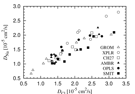
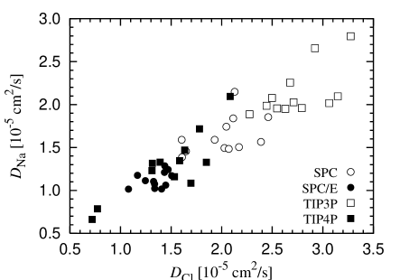
Figure 1: Diffusion coefficients $D_{\mathrm{Na}}$ and $D_{\mathrm{Cl}}$ for sodium and chloride, respectively. Left: Labelling according to the ionic force field. Right: Labelling according to the water model used.

In Sec. IV we present the results of our simulations, and show how the different force-fields differ in their description of the NaCl properties. One important conclusion can, however, be drawn already from Tab. 1: The parameters for the different water models (SPC, TIP3P and TIP4P) differ only slightly, representing the current good knowledge of the properties of water. For (aqueous) chloride, the differences are significantly larger, up to $10\,\%$ for the radius and up to $50\,\%$ for the depth of the attractive well of the Lennard-Jones interaction, reflecting the lack of high quality experimental input data. For (aqueous) sodium, there seems to be virtually no consensus on its properties. In the simulations, one can thus expect that the biggest differences will be in the Na–Na properties, followed by the Na–Cl interactions.

III Simulations

For this study, we decided to include the three most commonly used thermostats, namely Berendsen Berendsen et al. (1984), Nosé-Hoover Nosé (1984); Hoover (1985) and Langevin Grest and Kremer (1986). All of them are implemented into the Gromacs simulation software Lindahl et al. (2001) that was used for all of the computations presented in this paper. The target temperature was set to $298~{}\mathrm{K}$ and particle-mesh Ewald (PME) was used for long-range electrostatics. The pressure was held constant at $1~{}\mathrm{bar}$ using the Berendsen algorithm Berendsen et al. (1984).

For each combination of ionic force-field, water model and thermostat a MD simulation was run. In addition, for each combination of water model and thermostat a reference simulation without ions was done. The total number of simulations added up to 84. A pre-production analysis showed that the systems needed slightly less than $0.5~{}\mathrm{ns}$ to equilibrate. For each simulation run, we computed a $2~{}\mathrm{ns}$ trajectory and only the second half of that was included into the analysis.

The simulations were run at the physiological salt concentration of $0.87~{}\mathrm{mol}$. The simulation box contained slightly more than 10000 water molecules so that finite size effects are not expected. Lennard-Jones interaction was cut-off at $1~{}\mathrm{nm}$. The optimal choice for the cutoff length is not obvious and can vary between force fields (even between the ones for the ions and for water in the same simulation). For consistency, we decided to use the same cutoff in all simulations. For all of these systems, all relevant structures are on scales much smaller than $1~{}\mathrm{nm}$. Furthermore, all atoms are charged so that Lennard-Jones interactions quickly become negligible compared to electrostatic interactions, and the precise choice of cutoff does not matter as much as it does for other systems.

The simulations described above presented a significant numerical task, and a total of approximately 25 000 hours of cpu time was needed to complete them.

IV Simulation results

IV.1 Dynamic properties

The most common quantity to describe the dynamical behaviour of a system is its diffusion coefficient $D$. We have plotted the results for different forcefields and water models in Fig. 1. The format for this plot, as well as the following ones, is the following: All results are plotted twice, using two graphs next to each other. The data points in both graphs are identical but in the left figure we have labelled them (i. e., picked symbols for the data points) according to the ionic force field whereas in the right figure we have labelled them according to the water model used. This way it is easy to see whether there is any systematic dependence on the ionic force field and/or the water model.

Figure 2: Gibbs free energy of hydration for the different force fields per ion pair.

The results for diffusion coefficients using Berendsen and Nosé-Hoover were identical within statistical error, but using Langevin thermostat the diffusion coefficients were much smaller. Unlike the Berendsen and Nosé-Hoover thermostats, the Langevin thermostat is not momentum conserving, and thus we omit the results for the Langevin thermostat when computing the diffusion coefficients.

The results of our simulations are depicted in Fig. 1. The experimental values at infinite dilution are given by $D_{\mathrm{Na}}=1.334\cdot 10^{-5}~{}\mathrm{cm}^{2}/\mathrm{s}$ and $D_{\mathrm{Cl}}=2.032\cdot 10^{-5}~{}\mathrm{cm}^{2}/\mathrm{s}$ Marcus (1997). From the figure it is seen immediately that the dynamics is determined by the water model while the contribution of the ionic force field is negligible. The diffusion constant thus cannot be used to judge the quality of the different force fields. This is not surprising since in aqueous systems the behaviour is dominated by the water molecules as they outnumber the ions by a factor of order $100$. This is likely to be the case for other dynamic properties as well. A study of the dynamic properties of water models is beyond the scope and aim of this paper, and we refer to previous studies on this subject Wallqvist and Mountain (1999) and to the very informative webpage . To see the effect of the ionic force fields, we concentrate on static properties in the following.

IV.2 Gibbs free energy of hydration

The most frequently used way to compute free energies is by the “slow-growth” method, also known as Kirkwood’s coupling parameter method Kirkwood (1935) or as thermodynamic integration. The presence of solute in a solvent is determined by the parameter $\lambda$ that modifies the Hamiltonian $H$ of the system. $\lambda=0$ means that there is no interaction between solute and solvent whereas $\lambda=1$ means that the normal Hamiltonian for the combined system is used. The change of Gibbs free energy upon introducing the solute into the solvent is then given by

$$\Delta G=\int_{0}^{1}\left\langle\frac{\partial H}{\partial\lambda}\right\rangle d\lambda\;,$$ (3)

where the averages are taken at constant pressure. (If the averages are taken at constant volume, this equation would yield the change of free energy.) The advantage of this approach is that the change of (Gibbs) free energy is measured directly without the need to compute the (Gibbs) free energy of the solvent, thereby reducing the statistical error of the result. However, this method is computationally expensive since the integral has to be evaluated numerically by running simulations with different values of $\lambda$. While this is no significant problem when studying a single system, this is not feasible for a systematic study as presented in this paper.

A different way to compute the free energy of a system is given by

$$F=-k_{\mathrm{B}}T\ln\Bigl{\langle}\exp\bigl{(}-\frac{U}{k_{\mathrm{B}}T}\bigr{)}\Bigr{\rangle}\;,$$ (4)

with $U$ the potential energy of the system. This formula is easily understood by noting that it is conceptually identical to the computation of the chemical potential using insertion of a test particle, with the test particle being the entire system and the reference state being the vacuum. It offers the advantage that only a single simulation of the system with and without the solute is needed, not a large number of different simulations with gradually increasing $\lambda$. This formula is not as much used in the literature since for computing free energy differences it has to be applied twice to compute the free energies of the two comparison systems. The computed free energy difference then has a significantly larger statistical error, especially when only a small part of, for example, a large protein is mutated.

Figure 3: Typical examples from our set of radial-distribution functions for Na–Na, Cl–Cl and Na–Cl (from left to right). All curves were computed using the Berendsen thermostat.

We do not suffer from this problem as the number of ions is large enough to arrive at a statistically significant result. We thus apply Eq. (4) first to a simulation of aqueous NaCl and then to a simulation with the same number of water molecules (using the same water model and the same thermostat as in the first simulation) but without any ions. Since the two simulations are done at identical pressure and not at identical volume, the difference actually gives not the plain free energy but rather the Gibbs free energy $G$ of hydration.

The experimental values for the Gibbs free energy of hydration are $-347~{}\mathrm{kJ}/\mathrm{mol}$ for chloride and $-375~{}\mathrm{kJ}/\mathrm{mol}$ for sodium Marcus (1997), for a total of $-722~{}\mathrm{kJ}/\mathrm{mol}$. Older reported values are $-363~{}\mathrm{kJ}/\mathrm{mol}$ for chloride and $-406~{}\mathrm{kJ}/\mathrm{mol}$ for sodium Cotton and Wilkinson (1972). It is assumed that isolated ions are to be hydrated, i. e., the crystal lattice of solid NaCl does no longer need to be broken up. (These two different concepts are frequently referred to as “hydration” versus “solvation”.) It should be stressed that all those experimental values are at infinite dilution, i. e., all mutual interactions among the ions in the aqueous phase are ignored.

The numerically computed Gibbs free energies $G$ are depicted in Fig. 2. Since we used three different thermostats, this resulted in three different values for $G$ for each combination of ionic forcefield and water model. We use those three different values to compute an error estimate that is marked by the error bar in the figure. Most of the error bars are that small that they hardly can be seen, confirming that application of Eq. (4) is sufficient for this system.

The experimental data given above for the Gibbs free energy of hydration is at infinite dilution and thus needs to be corrected to account for the finite molarity of physiological systems as treated in the simulations. We were unable to find direct experimental data for the enthalpy change of dilution but this quantity can be computed from the difference in the enthalpy of solution for the two different concentrations. For the parameters in question, the experimental values Beggerow (1976) lead to a correction of $-2~{}\mathrm{kJ}/\mathrm{mol}$.

All numerically computed data in Fig. 2 are more negative than the experimental data. This means that either the attractive mutual interaction of the ions is overestimated in the simulations, or that the shielding of that interaction due to the water is underestimated. It should be stressed that the parametrisation of all ionic force fields was done at infinite dilution, meaning that only a single ion was considered. The effect of finite concentration was thus not considered in the parametrisation process. A systematic numerical study of the concentration dependence of the Gibbs free energy of hydration could help to provide an understanding but no such study seems to have been published so far. Comparing experiment and the simulation results in Fig. 2 allows to judge the agreement between a force field and experiment — for precisely the molarity studied in this paper — but the picture might be completely different at other molarities.

IV.3 Radial-distribution functions

Next, we compare the radial-distribution functions (rdf). There are three kinds of particles in the simulation, namely Na, Cl and water, resulting in six different pairs and thus six different radial-distribution functions. For the purpose of computing the rdf’s, the position of the oxygen atom is taken to represent the entire water molecule, and we will thus use the label “O” for water. For space reasons we will not discuss the water-water rdf’s in the following. This is no relevant limitation since for the physiological concentrations they depend hardly on the ionic force field. (The complete set of rdf’s can be found as supplementary material at our website .)

In Fig. 3 we present the rdf’s for four different force field combinations. (For the complete set, see the supplementary material.) It is immediately obvious that the rdf’s differ from each other in many aspects, such as the number of peaks, the relative and absolute heights of the peaks, and that those differences are significant.

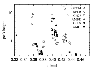
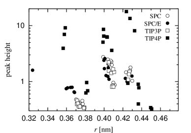
		Na–Na
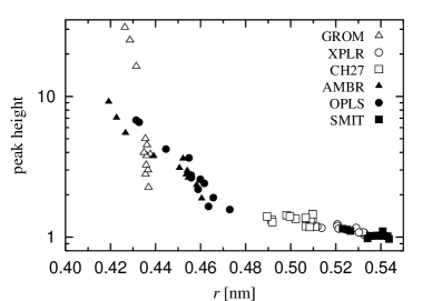
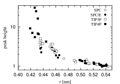
		Cl–Cl
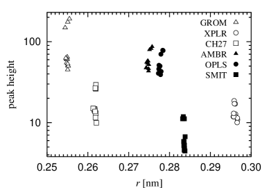
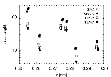
		Na–Cl
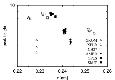
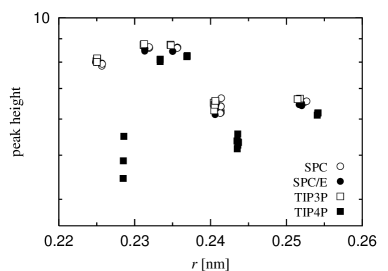
		Na–O
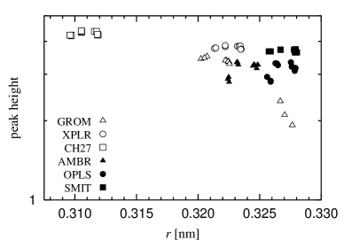
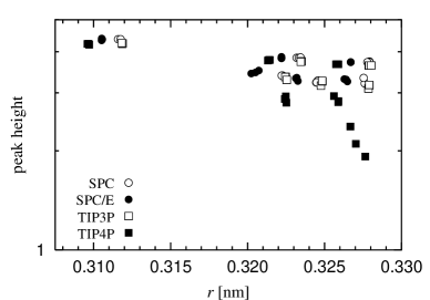
		Cl–O

Figure 4: Position and height of the first peak of the radial-distribution function for (from top to bottom) Na–Na, Cl–Cl, Na–Cl, Na–O (i. e., water) and Cl–O.

It would be impossible to present all rdf’s by directly plotting them. To give a more systematic overview in a condensed way, we have computed the position and height of the first peak for all rdf’s. For this, a Gaussian is fitted to the rdf in the neighbourhood of the peak. The results are depicted in Fig. 4. We first will discuss the simulation results and will then put them into the context of experimental results.

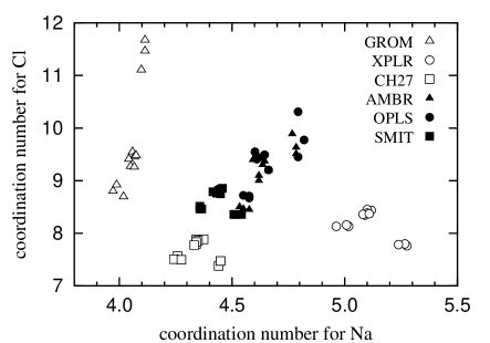
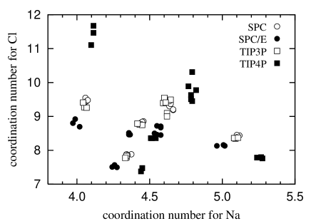
Figure 5: Coordination number, computed by integrating the radial-distribution function between the water oxygen and the ion from zero up to its first minimum.

From Fig. 4 it is seen that the Na–Na and Cl–Cl peaks are scattered widely (Na–Na being scattered more than Cl–Cl), and that there is no well-defined systematic tendency. This is the case for both the position and the height of the peak. Also for the Na–Cl results, the peaks are scattered widely but we want to point out one curiosity: While for the Na–Na and Cl–Cl peaks there is a dependence both on the ionic force field and the water model, the position of the Na–Cl peaks is independent of the chosen water model. An easy explanation could be that sodium and chloride ions are frequently in direct contact with each other so that the properties of the water model are of minor importance.

The positions of the Na–O and Cl–O peaks differ less between force fields. (Please observe the different scale of the $r$-axis in the different subfigures.) The height of the peaks, in contrast, still varies by about a factor $3$ between the different force fields.

We will now discuss these findings in the context of experimental limitations. Radial-distribution functions can, in principle, be measured by x-ray diffraction since they are related to the Fourier transformation of the structure factor. To get a strong enough signal, the substances have to be of sufficiently high concentration. This makes the experimental determination of Na–Na, Na–Cl or Cl–Cl rdf’s impossible.

For Na–O and Cl–O rdf’s, the signal is only weak at physiological concentrations. It is possible to determine the position of the peak of the rdf quite well since it is directly related to the wave length of the peak of the structure factor. The height of the peak of the rdf, however, can be measured only with great difficulty. (We will return to this in the next section, when discussing the coordination number.) We should add that for sodium any kind of measurement is more difficult than for chloride since there exists only a single isotope of sodium, and consequently the difference method of isotope substitution cannot be used.

Determining suitable experimental values for the peak positions is aided by the experimental observation that they depend only very weakly on molarity of the salt. Surprisingly, the results for crystals and aqueous solutions are also very similar. Marcus Marcus (1997) quotes values between $0.233~{}\mathrm{nm}$ and $0.240~{}\mathrm{nm}$ for the Na–O peak position but earlier reviews include values up to $0.25~{}\mathrm{nm}$ Marcus (1988). For chloride, the quoted values are between $0.30~{}\mathrm{nm}$ and $0.32~{}\mathrm{nm}$ Marcus (1997). Other values quoted in the literature are within these limits, except that also a Cl–O peak position of up to $0.335~{}\mathrm{nm}$ is reported Enderby and Neilson (1979).

The simulation results in Fig. 4 are now easily understood. There are only two quantities that are susceptible to (decent-quality) measurement, namely the peak positions of the Na–O and Cl–O rdf’s. Consequently the predicted values for these two quantities vary only little between force fields. Taking the entire range of experimental values (i. e., not deciding by some criterion that one experimental value is “better” than the others), all force fields basically reproduce the experimental knowledge.

The huge spread observed in the other peak positions and in all the peak heights in Fig. 4 is simply an echo of the lack of experimental data for these important structural quantities, and no empirical force field can be better than the available experimental data. Any method that relies on mutual peak position of the ions therefore faces a problem, and no solution to this problem is in sight.

IV.4 Coordination number

A different description of the water structure around the ions is given by the coordination number. Technically this quantity is computed by first determining the location of the first minimum of the radial-distribution function and then integration the radial-distribution function from zero up to this point,

$$n_{\mathrm{coord}}=\frac{4\pi}{V_{\mathrm{water}}}\int_{0}^{r_{\mathrm{min}}}dr\,r^{2}g(r)\;,$$ (5)

where $V_{\mathrm{water}}$ is the volume of one water molecule. The geometric meaning of $n_{\mathrm{coord}}$ is that it gives the number of solvent molecules in the first hydration shell around the ion. It should be noticed that the coordination number is a purely geometrical quantity, and it does not imply that this number of water molecules is influenced in some way by the ion.

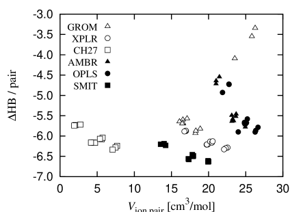
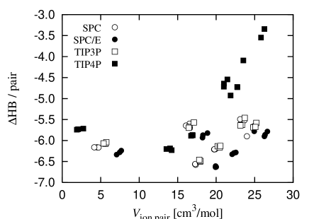
Figure 6: Apparent molar volumes of the ions, and the change of the number of hydrogen bonds per ion pair. (The latter quantity is negative, meaning that hydrogen bonds are destroyed by the ions.)

Experimental data on the coordination number is scarce. The reason for this is twofold: First, the amplitude of the radial-distribution function is difficult to measure. The amplitude of $g(r)$ cannot directly be inferred from the structure factor at the corresponding wave length but only follows indirectly from the normalisation condition $g(r)=1$ for $r\to\infty$. Secondly, the position of the first minimum is less well-defined than the position of the first peak, and it is not always immediately obvious where to stop the integration. (This can already be seen from the examples of simulational rdf’s in Fig. 3).

The coordination numbers computed from our simulations are displayed in Fig. 5. First, the position of the first minimum was computed. For space reasons we decided against displaying these intermediate results and only show the resulting coordination numbers. (The positions of the first minimum are between $0.305~{}\mathrm{nm}$ and $0.34~{}\mathrm{nm}$ for Na–O, and between $0.375~{}\mathrm{nm}$ and $0.44~{}\mathrm{nm}$ for Cl–O.)

The reported experimental coordination numbers for sodium are between $4$ and $8$ Marcus (1988). For chloride, the same source gives values for chloride of around $6$ when measured for NaCl solutions but there are only few of those measurements. The coordination number of chloride should change only slightly when the sodium is replaced by some other cation. This should allow us to use also data for other salts, thereby getting better statistics. However, if this is done coordination numbers as high as $11$ can be included Enderby and Neilson (1979). Given the large spread of the experimental values, the coordination number is not well suited to quantify the agreement between experiment and molecular dynamics simulations.

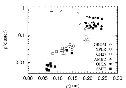
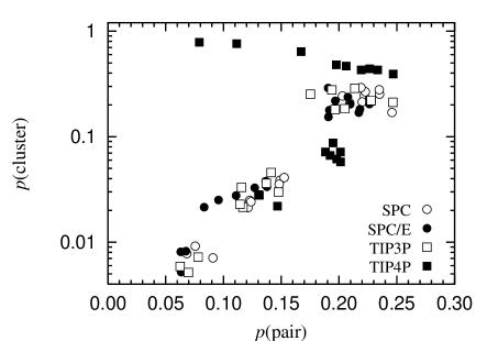
Figure 7: Ratio $p(\mathrm{pair})$ of all particles that are in a cluster consisting of two particles, and ratio $p(\mathrm{cluster})$ of particles that are in a cluster consisting of three or more particles.

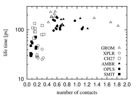
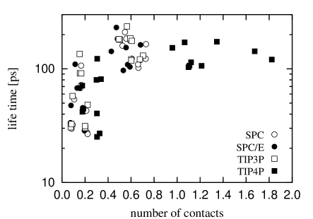
Figure 8: Life time of a contact between a cation and an anion, as well as the mean number of contacts that each ion has.

IV.5 Molar volumes

Each ion occupies a certain volume determined by its radius. This quantity is of little practical relevance, however, since the introduction of the ion changes the local structure of the surrounding water, and thus also the local density. These effects are included in the quantity known as molar volume. If the local compression of the water overcompensates the steric volume of the ion, the molar volume can become negative.

The experimental molar volumes are $-6.7~{}\mathrm{cm}^{3}/\mathrm{mol}$ for sodium and $23.3~{}\mathrm{cm}^{3}/\mathrm{mol}$ for chloride Millero (1971); Akitt (1980); Marcus (1997). This gives a volume of $16.6~{}\mathrm{cm}^{3}/\mathrm{mol}$ per ion pair.

In a simulation using pressure coupling, the molar volume per ion pair can directly be computed by determining the average size of the simulation box, and from this subtracting the average size of the simulation box of a simulation of pure water. (It is essential to use the same water model and the same thermostat in both simulations.) This gives the molar volume per ion pair depicted in Fig. 6. Comparison with the experimental values shows that Charmm-27, OPLS and Amber are performing a little bit less well in this test as do the other force fields.

IV.6 Hydrogen bonding

Most ions are known to break the hydrogen bond network of the water around them. This can be explained by the water molecules aligning themselves for better interaction with the ion, at the expense of breaking the hydrogen bonds toward other water molecules. (On average, a water molecule has about $1.55$ hydrogen bonds in bulk water.) Experimental values for $\Delta\mathrm{HB}$, the change in the number of hydrogen bonds due to one ion, is $-0.03$ for sodium and $-0.61$ for chloride Marcus (1994, 1997).

We have computed the change in the number of hydrogen bonds by comparing two simulations, one with and one without the ions. Classical MD can only give an estimate of the number of hydrogen bonds, by counting the number of potential acceptors and donors that fulfil certain geometric conditions. The result is depicted in Fig. 6. It is immediately seen that all forcefields yield values for $\Delta\mathrm{HB}$ that are much more negative than the experimental values.

An easy explanation can be offered for this observation. All force fields discussed in this paper do not include explicit energy terms for hydrogen bonds. Rather, hydrogen bond interaction is integrated out and is included in the partial charges inside the water molecule. This approach works very well if the water molecules are arranged in the same way as in bulk water. In any other arrangement, e. g. if ions are introduced, they are now easier to rotate as no hydrogen bond energy terms need to be broken.

IV.7 Cluster analysis

Next we discuss the physical background behind the peaks in the ionic rdf’s in Fig. 4. For the Na–Cl interaction a large peak is expected since the two ions are of opposite charge. For the Na–Na and Cl–Cl rdf’s, this explanation does not hold. Especially if the peak is significantly higher than $1$, this means that ions “like” to be at a certain distance from each other much more than to be away from each other as much as possible — even though they are strongly repelling each other through electrostatic forces. In earlier simulations of aqueous ionic systems pairing of chloride ions was found but it was later realised that this pairing is an artifact that disappears if long-range electrostatic forces are treated properly Perera et al. (1994); Buono et al. (1994); Hummer (1993).

Such problems can be ruled out here but there still is the question whether clusters of ions exist. In such a cluster, several cations (anions) can be close to each other because their mutual repulsion is compensated by the simultaneous presence of several anions (cations). For this reason we have performed a cluster analysis. We define a cluster as the set of all ions that are connected by distances of $0.35~{}\mathrm{nm}$ or less. From the radial-distribution functions in Fig. 4 it can be seen that $0.35~{}\mathrm{nm}$ is a reasonable value, and that the precise choice does not effect the results.

Figure 9: Effective potentials for the same simulations as depicted in Fig. 3. The product of the effective potential $V_{\mathrm{eff}}$ and the Boltzmann factor $\beta\equiv 1/(k_{\mathrm{B}}T)$ is unitless.

After doing this, we collected statistics on the number of ions in each cluster, computing the ratio $p(N)$ of ions that belong to a cluster consisting of $N$ ions. In Fig. 7 we have plotted $p(\mathrm{pair})\equiv p(2)$ and $p(\mathrm{cluster})\equiv\sum_{n=3}^{\infty}p(n)$. It can be seen that the different forcefields result in a large span for the results, and the probability for clusters of three or more particles spans more than two orders of magnitude.

The different tendency for cluster formation is reflected also in the mean number of contacts that each ion has. This quantity is depicted in Fig. 8. Also depicted in this figure is the mean life time of each contact. This shows that if the life time is small, the mean number of contacts is also small but a large life time does not necessarily imply a large number of contacts. This can be explained by the interplay between the time scale for breaking a contact (i. e., the life time) and the time scale needed by two partners to find each other.

IV.8 Implications for the effective potential

The radial-distribution function can be used to define different potentials. The most common one is the potential of mean force $V_{\mathrm{PMF}}$, defined by

$$g(r)=\exp[-\beta V_{\mathrm{PMF}}(r)]\;.$$ (6)

Although not immediately visible in the formula, the potential of mean force includes the direct interaction between two particles at fixed positions, and additionally the contribution from having a third particle at a fixed position provided particles 1 and 2 are already fixed Hansen and McDonald (1986). In other words, the potential of mean force includes first order corrections to the pure pairwise potential. Differences in $g(r)$ directly translate into differences in $V_{\mathrm{PMF}}(r)$.

If higher order corrections are included, a different kind of potential is found, termed effective potential $V_{\mathrm{eff}}(r)$ Lyubartsev and Laaksonen (1995). The effective potential is defined by the condition that in the canonical ensemble it yields the desired radial-distribution function. Under the restriction that the Hamiltonian can be written as a sum of two-particle terms, the effective potential always exists and is uniquely defined (up to a physically irrelevant offset). If the full set of rdf’s is used for this process, the original microscopic potential is recovered.

The value of the effective potential lies in that it allows one to integrate out degrees of freedoms. This process is referred to as coarse-graining. Of particular interest is to integrate out the solvent since this decreases the number of particles and thus the computational burden by approximately a factor $100$. Aim is thus to find three effective potentials, namely for Na–Na, Na–Cl and Cl–Cl interaction, that, when used in a MC or MD simulation without a solvent, reproduce the microscopic rdf’s for Na–Na, Na–Cl and Cl–Cl computed including the solvent.

As initial guess for $V_{\mathrm{eff}}(r)$, the potential of mean force from Eq. (6) is used. From the guessed effective potentials, the rdf’s are computed in an MC simulation. If the rdf for particles of type $i$ and $j$ at distance $r$ is larger (smaller) than the microscopic target rdf, the guess for $V^{(i,j)}_{\mathrm{eff}}(r)$ is decreased (increased). This process is repeated until convergence is achieved. More sophisticated methods that use the four-particle correlation function to compute an improved guess for the effective potential have been developed under the name inverse Monte-Carlo Lyubartsev and Laaksonen (1995) but they are not numerically stable enough for this problem.

The effective potential for the rdf’s from Fig. 3 are shown in Fig. 9. It is instructive to compare these two figures since it demonstrates the difference between the potential of mean force and the effective potential. The Cl–Cl radial-distribution functions of both Gromacs+SPC and X-plor+TIP3P have a peak. According to Eq. (6) this translates into a dip in $V_{\mathrm{PMF}}$. For $V_{\mathrm{eff}}$, this dip is almost invisible for X-plor+TIP3P. This means that the peak in $g(r)$ is (almost) solely due to interaction with particles that were not integrated out. In other words: Two chloride ions have a tendency to be close to each other due to attractive interaction with the same sodium ion. For Gromacs+SPC, $V_{\mathrm{PMF}}$ contains a big dip for the Cl–Cl interaction. This means that a big contribution to the peak in $g(r)$ comes from interactions that have been integrated out, namely the water molecules.

The important conclusion, however, is that not only the structure of the ionic solution, as given by $g(r)$, depends heavily on the force field used. Also the effective potentials show a large variation on the precise force field parameters.

V Conclusions

In this paper, we have compared different force fields describing aqueous NaCl. To this end, we have computed several quantities, some of them of a thermodynamic origin but being of structural nature. We can divide the computed quantities into two groups. In the first group are the quantities that have an experimental counterpart that is easily measurable. All force fields reproduce most of those values sufficiently well. In the second group are the quantities for which there exists no or very limited experimental data. The different force fields predict vastly different values for those quantities.

The Gibbs free energy of hydration is the most basic thermodynamic quantity for describing aqueous ionic solutions. It is a “purely thermodynamic” quantity if and only if the system is in the dilute limit. For finite concentration of ions, the mutual interaction of ions becomes important, and thus the structural properties of the ions enter. Comparison of experimental and our simulational values for the Gibbs free energy of hydration shows that the difference between those values depends on the force field used, so in principle it can be used to judge the suitability of a force field for application at physiological salt concentrations. While the Gibbs free energy of hydration is an important fundamental thermodynamic property, its importance in most molecular dynamics simulations might be limited, however, since the ions are usually kept hydrated during the entire simulation.

Structural properties are often more important, best described by the radial-distribution function. The position of the first peak of the radial-distribution functions for sodium–water and chloride–water is characteristic for the first hydration shell of those ions. All force fields reproduce the experimental values sufficiently well. This means that all force fields are able to describe well those physical effects that are governed by the hydration properties in the immediate neighbourhood of the ions.

For the ion–ion radial-distribution functions it was shown that the different force fields lead to significantly different results. Since there exists no experimental data for those properties, this does not imply that a few (or all) force fields were developed improperly but simply reflects the limited knowledge of such properties. The predictive power of any model for aqueous NaCl thus is very limited if structural properties of mutual ion interaction are important. In particular this means that greatest care should be taken if the radial-distribution functions are used as input for some other application.