Boundary processing for Monte Carlo Simulations in the Gap-Tooth Scheme.

Abstract

This note reports on a scheme for interpolating the boundary conditions between non-adjacent modeling regions when the model is based on Monte-Carlo computations of a collection of particles. The scheme conserves particles in a natural way, and thereby can be made to conserve other quantities.

Keywords Particle models, equation-free computation, conservation

1 Introduction

In Kevrekidis’s gap-tooth scheme[1] which permits macro-scale computation over large regions from microscopic models computed over small regions (the teeth), it is necessary to generate the boundary conditions for each tooth from the solutions in neighboring teeth by a suitable-order interpolation.

The gap-tooth scheme can be applied to initial-boundary values problems for evolutionary PDEs. In it, space is partially “tiled” by non-adjacent boxes, called teeth, as shown in Figure 1 for one space dimension. The time-dependent, microscopic computational model is solved only inside the teeth, while the solution between the teeth is obtained by interpolation between the teeth based on smoothness assumptions.

A solution of the model inside the teeth requires appropriate boundary conditions on the sides of each tooth. Edge teeth (those adjacent to a boundary of the actual problem) have part of their boundary specified from the problem, as shown in Figure 1. The other boundaries are the ones for which the conditions must be generated.

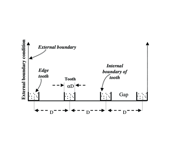
Figure 1: Teeth partially tiling a region of space

Depending on the model used inside the teeth, the variables interpolated between the teeth might be the same variables, or might be a restriction of them to a lower-dimensional set of variables, the coarse variables, as described in [2]. If the variables inside the teeth are interpolated between teeth, then the results of those interpolations can be used directly for the boundary conditions (e.g., the fluxes might be interpolated, as illustrated in [1]).

However, the main point of modeling over the small teeth is to use microscopic models in their interior (such as particle models of fluids or reacting mixtures) in which case the restriction to the macroscopic (coarse) variables interpolated between the teeth is to low-order moments of the solution in each cell, such as density, etc. If the boundary conditions have to be generated from these interpolants, it is necessary to use an appropriate computational interface at the boundary between the restricted coarse variables outside the teeth and the internal microscopic variables inside the teeth.

In this note we propose a scheme for interpolating boundary conditions in Monte-Carlo-like particle simulations that is particle-based and avoids the restriction operation and the resulting boundary interface issues. The restriction operation is then necessary to compute the macroscopic description but not for the far-more-frequently computed boundary conditions..

2 Linearly-interpolated Particle Boundary Conditions

When we simulate a system in terms of interacting “particles,” each with a spatial position and possibly additional state variables (such as velocity, charge, etc.) over a continuum in space, the “data” crossing any “boundary” between two spatial regions (i.e. any arbitrary $n-1$ dimensional surface diving the $n$-dimensional space into two different regions) is a “discrete flux” consisting of particles crossing that boundary from time to time in either direction, carrying with them their additional state variables such as velocity and so on. In macroscopic variable we will typically characterize these in terms of the total flux, or velocity, or pressure, or some combination of these and other moments of particle state variables. If we are performing a microscopic simulation over the whole of the spatial domain, there is never any need to “map” between the microscopic boundary conditions and the macroscopic variables except possibly at the external boundaries where the microscopic boundary conditions might be handled by such devices as absorbing boundaries, reflecting boundaries, or periodic boundaries. However, when we use the gap-tooth scheme, each additional tooth introduces $2^{n}$ additional internal boundaries (where $n$ is the space dimension).

In a particle simulation, we can identify two fluxes for each particle type at a boundary - the outgoing flux of particles leaving the tooth, and the incoming flux of particles entering the tooth. The outgoing flux is naturally generated by the microscopic simulation - in each simulation time step some number of particles inside a tooth cross a boundary and are “lost to that tooth.” The incoming flux has to be generated at a boundary as an implementation of the boundary condition for the microscopic simulation in each tooth. Figure 2 shows two neighboring teeth and some of the incoming and

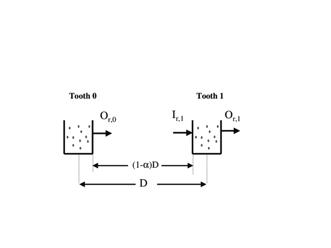
Figure 2: Input and output right-going fluxes from teeth

outgoing fluxes. We have named the outgoing flux from tooth $i$ as ${\rm O}_{d,i}$ where $d$ is $r$ or $l$ for right-going or left-going flux, respectively. (In $n$ space dimensions there would be $2n$ outgoing fluxes from each tooth.) The incoming fluxes are named ${\rm I}_{d,i}$. If there were no gaps (i.e., $\alpha=1$) the unknown incoming flux in a particular direction to one tooth would simply be the known outgoing flux in the same direction from the adjacent tooth, i.e.,

$${\rm I}_{r,i+1}={\rm O}_{r,i}$$

and

$${\rm I}_{l,i}={\rm O}_{r,i+1}$$

When we have a gap, it seems natural to interpolate for ${\rm I}_{r,i}$ from the nearest ${\rm O}_{r,j}$, that is, from ${\rm O}_{r,i-1}$ and ${\rm O}_{r,i}$, and similarly for the flux in the other direction(s). Using linear interpolation, we have:

$${\rm I}_{r,i}=\alpha{\rm O}_{r,i-1}+(1-\alpha){\rm O}_{r,i}$$

and

$${\rm I}_{l,i}=\alpha{\rm O}_{l,i+1}+(1-\alpha){\rm O}_{l,i}$$

where $\alpha$ is the ratio of the tooth width to the center spacing of the teeth. (In this note, we will discuss only equally-spaced, equally-sized teeth, although a practical code will almost certainly need to change the spacing according to the solution behavior.)

In a particle simulation, the outgoing flux is not a real-valued quantity but, depending on the form of the simulation, either a discrete-valued quantity - corresponding to the number of particles that have crossed the boundary in a simulation step if the simulation proceeds in a sequence of prescribed-length time steps, or a series of “impulse” functions - if the simulation is “event-oriented” and proceeds to the next event (which could be a particle-particle interaction or a boundary crossing). So what do we mean by an interpolation between such variables? Looking at Figure 3 we note that we have the following expressions for the inputs

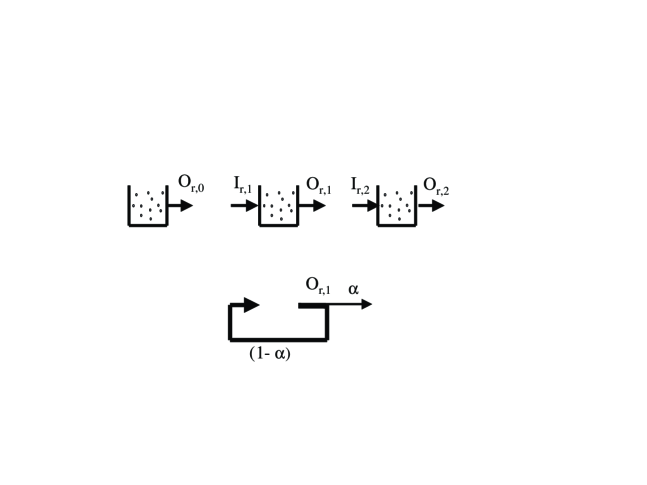
Figure 3: Linear interpolation of input fluxes by redirection of output fluxes

${\rm I}_{r,1}$ and ${\rm I}_{r,2}$:

$${\rm I}_{r,1}=\alpha{\rm O}_{r,0}+(1-\alpha){\rm O}_{r,1}$$

$${\rm I}_{r,2}=\alpha{\rm O}_{r,1}+(1-\alpha){\rm O}_{r,2}$$

Thus, the $\alpha$ of the output ${\rm O}_{r,1}$ contributes to ${\rm I}_{r,2}$ and $(1-\alpha)$ of it contributes to ${\rm I}_{r,1}$. In other words, we can interpret these equations in a stochastic sense and send $\alpha$ of the particles leaving a tooth to the right to the left end of the right neighbor, and the remaining $(1-\alpha)$ back into the left end of the itself, as shown in the lower part of Figure 3. The left-going outputs can be treated similarly. Thus boundary conditions for the internal teeth boundaries are handled directly at the particle level. We call this a flux redirection scheme. This one is based on linear interpolation. Note that this approach preserves the number of particles - and will also preserve any other conserved values carried by the particles.

The way in which the external boundaries are handled necessarily depends on the specified boundary conditions. If, for example, an external boundary is reflecting, one way to handle it is to place an edge tooth centered on the boundary as shown in Figure 4. Only the

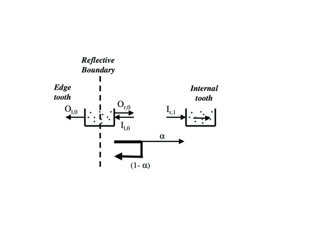
Figure 4: Handling a reflective boundary by flux redirection

right half of the tooth need be simulated since the assumption is that the left half is its mirror image and the external boundary can be handled as reflecting. However, we still have to get a value for ${\rm I}_{l,0}$ since for internal boundaries it would depend in part on the unknown ${\rm O}_{l,0}$. However, the reflecting condition means that we can use ${\rm O}_{r,0}$ for the value of ${\rm O}_{l,0}$. this is simply handled by reflecting $(1-\alpha)$ of the output from the right boundary of tooth 0 back in, and sending the remaining $\alpha$ onto tooth 1 as part of its right-going input to its left boundary, as shown in the lower part of Figure 4. Note that this external boundary scheme also preserves the number of particles and other conserved values carried by the particles at this boundary.

2.1 A Trivial Example

Consider the linear equation

$$\frac{\partial u}{\partial t}+\frac{\partial u}{\partial x}=0$$ (1)

where $u(x,t)$ is a smooth approximation to the local “density” of a collection of particles. While we shouldn’t be using computer time on such a simple problem, we can simulate it by moving each particle a distance $\Delta$ to the right in each time step of length $\Delta$. Now suppose that we are doing this using teeth that occupy a fraction $\alpha$ of the spatial domain. For convenience, consider a time step of size $\alpha D$. (Other time steps will give the same result, but would require a more complex discussion.) Hence, in one time step, all of the particles in each tooth move from their current positions to positions $\alpha D$ to the right - outside of the tooth they came from. Hence, $\alpha$ of them should move to the neighboring tooth to the right - by being moved a further distance $(1-\alpha)D$ - and $(1-\alpha)$ of them should be moved back to the originating tooth - by being moved left an amount $\alpha D$. (If the time step were longer than $\alpha D$ some of the particles so moved would still be outside of the destination tooth and would have to be subject to the same rule again. In effect, a larger time step would be handled as a number of time steps of length $\alpha D$ followed by one shorter time step.)

Let us look at the equation for the particle density, where the density is simply approximated as a constant over the tooth and determined by the number of particles in the tooth (modulo some scaling which is not important in this example.) We will denote the density in tooth $i$ and time step $n$ as $u_{i,n}$. We have (within the rounding resulting from the fact that we are dealing with integral numbers of particles)

$$u_{i,n+1}=(1-\alpha)u_{i,n}+\alpha u_{i-1,n}$$

or

$$u_{i,n+1}-u_{i,n}=-\alpha(u_{i,n}-u_{i,n-1})$$

which is precisely an upwind finite difference approximation to eq. (1) with $\Delta t/\Delta x=\alpha$ which, since $\Delta x=D$, is consistent with $\Delta t=\alpha D$.

3 Higher-order Boundary Conditions and “Anti Particles”

The method discussed above uses linear interpolation. This is adequate in some cases, but not others. Consider the heat equation

$$\frac{\partial u}{\partial t}=\nu\frac{\partial^{2}u}{\partial x^{2}}$$ (2)

This is the asymptotic solution of a simulation of a number of particles subject to a suitable random walk as the number of particles goes to infinity. We could (if we wanted to waste computer cycles) simulate it by taking a collection of particles in space and, at each of a sequence of time steps, taking half of the particles (picked at random or by some means that doesn’t bias the result such as every other one in spatial ordering) and moving them left a distance $r$ and moving the other half right the same distance. The distance they should be moved is proportional to the square root of $\Delta t$ and $\nu$, namely

$$r=\sqrt{2\nu\Delta t}$$ (3)

so that $r$ is the standard deviation of the distribution. (With this “binary” walk the asymptotic convergence to the solution of the heat equation is also in terms of the time step going to zero. If each particle were subject to an independent Gaussian movement with mean zero and standard deviation $r$, the result would be independent of the time step, but we will use the binary walk for ease of discussion.)

What happens if we use the scheme from the previous section and apply the simple analysis above to it? Again, let us choose a time step such that $r=\alpha D$. In each time step, half of the particles will exit a tooth to the left and half to the right. If we use the flux redirection scheme based on linear interpolation we will get the approximate equation for $u_{i,n}$:

$$u_{i,n+1}=(1-\alpha)u_{i,n}+\alpha(u_{i-1,n}+u_{i+1,n})/2$$

which is a finite difference approximation to eq. (2) if $\alpha=2\nu\Delta t/\delta x^{2}$, but this requires that

$$r=\alpha D=2\nu\Delta t/D$$ (4)

This gives a different value of $r$ that that given in eq. (3). The reason is that linear interpolation is not adequate for the boundary condition in this case. Diffusion is dependent on the derivative of the flux, not on its actual level, so we need at least a second-order interpolant.

Referring back to Figure 3 we could do quadratic interpolation on the three values ${\rm O}_{r,i}$, $i=0,1,2$ to estimate either ${\rm I}_{r,1}$ or ${\rm I}_{r,2}$. Using the former, we have

$${\rm I}_{r,1}=\frac{\alpha(1+\alpha)}{2}{\rm O}_{r,0}+(1-\alpha^{2}){\rm O}_{r,1}-\frac{\alpha(1-\alpha)}{2}{\rm O}_{r,2}$$ (5)

Note that the coefficient of the last term is negative. Any higher-order interpolant has to have some negative coefficients (which accounts for their poor properties near sharp fronts). We note that with the quadratic interpolation in eq. (5) the following fractions of the output ${\rm O}_{r,1}$ should be sent to the inputs:

• $(1-\alpha^{2})$ to ${\rm I}_{r,1}$

• $\alpha(1+\alpha)/2$ to ${\rm I}_{r,2}$

• $-\alpha(1-\alpha)/2$ to ${\rm I}_{r,0}$

This raises the issue of how to move a negative number of particles from the output of one tooth to the input of a neighboring tooth. We propose sending “anti particles,” namely, particles whose state is the negative of the state of a regular particle, and which will annihilate a regular particle later. (In the heat equation model, the only state of a particle is its existence - which could be viewed as its unit mass. If a particle also had other state variables such as momentum, the anti particle would have the same velocity, but because of its negative “mass” its momentum would be the reverse. In the simulations we have done, an anti particle is annihilated by the nearest particle after the completion of the time step. If it also carried momentum, it would be necessary to move any excess or deficit momentum after the mutual self destruction of two particles to another neighboring particle.) With this model, we can use direction of right-going output flux in second order interpolation as shown below:

• Send $(1-\alpha(1+\alpha)/2)$ of the particles to the input of the same tooth

• Send $\alpha^{2}$ of the particles to the input of the right neighbor

• Send the remaining $\alpha(1-\alpha)/2$ of the particles to the right neighbor, send copies of them to the same tooth, and send anti-particle copies of them to the input of the left neighbor.

Note that the sum of the number of particles (where anti-particles are negative in the count) is unchanged so there is preservation of “mass” and other conserved values.

We now return to the heat equation example. With $r$ equal to $\alpha D$ as before, we now find that we get the finite difference equation

$$u_{i,n+1}=(1-\alpha^{2})u_{i,n}+\alpha^{2}(u_{i-1,n}+u_{i+1,n})/2$$

which is the finite difference approximation to the heat equation with $\alpha^{2}=2\nu\frac{\Delta t}{\Delta x^{2}}$. Noting that $r=\alpha D$ and $\Delta x=D$ we see that

$$r=\sqrt{2\nu\Delta t}$$

agreeing with eq. (3).

4 Comments

The key ideas in this note are the redirection of the outward fluxes based on the spacing of the teeth, and the use of “anti particles” to handle negative interpolation coefficients. The ideas go over to higher dimensions in which a particle may exit a tooth from one or several boundaries. All that is necessary is to do the redirection in each space dimension separately, so that the particle could move to any one of the $3^{n}-1$ nearest neighbors in $n$ dimensions (or more distant neighbors if even higher order interpolation is needed). While we have conserved the number of particles with the schemes discussed, a wider range of schemes can be considered if this feature is dropped. Dropping conservation may be necessary to handle a non-uniform mesh (although are ways to maintain conservation by using more inputs in an interpolation than necessary, but this issue has not been fully explored).

References

- [1] Kevrekidis, I. G., Coarse Bifurcation Studies of Alternative Microscopic/Hybrid Simulators, Plenary Lecture, CAST Division of the AIChE, AIChE Annual Meeting, Los Angeles, 2000, slides at http://arnold.princeton.edu/ yannis/
- [2] Equation-Free Multiscale Computation: enabling microscopic simulators to perform system-level tasks, NEC research Institute Report 2002-010N, Aug, 2002, Submitted to Communications in the Mathematical Sciences (with I. G. Kevrekidis, J. M. Hyman, P. G. Kevrekidis, O. Runborg, and C.Theodoropoulos) at http://www.neci.nj.nec.com/homepages/cwg/