Improving efficiency of supercontinuum generation in photonic crystal fibers by direct degenerate four-wave-mixing

Abstract

We numerically study supercontinuum (SC) generation in photonic crystal fibers pumped with low-power 30-ps pulses close to the zero dispersion wavelength 647nm. We show how the efficiency is significantly improved by designing the dispersion to allow widely separated spectral lines generated by degenerate four-wave-mixing (FWM) directly from the pump to broaden and merge. By proper modification of the dispersion profile the generation of additional FWM Stokes and anti-Stokes lines results in efficient generation of an 800nm wide SC. Simulations show that the predicted efficient SC generation is more robust and can survive fiber imperfections modelled as random fluctuations of the dispersion coefficients along the fiber length.

I Introduction

After the first observation of a 200-THz supercontinuum (SC) spectrum of light in bulk glass[1, 2], much has been done on the understanding and control of this process[3]. A target of numerous experimental and theoretical investigations has been the improvement of the characteristics and simplification of the technical requirements for the generation of a SC[3]. The first experiments in bulk materials, based on self-phase modulation (SPM), required extremely high peak powers ($\rm{>10MW}$).

New techniques based on the use of optical fibers as a nonlinear medium for SC generation allowed lower peak powers to be used due to the long interaction length and high effective nonlinearity[4, 5, 6, 7]. However, the necessity to operate near the wavelength for zero group velocity dispersion, restricted the SC generation to the spectral region around and above $\rm{1.3\mu m}$. The use of dispersion-flattened or dispersion-decreasing fibers as nonlinear media for SC generation resulted in a flat SC spanning 1400-1700nm[8, 9] and 1450-1650nm[10], respectively. The spectrum was still far from the visible wavelengths and in some cases very sensitive to noise in the input [10].

Photonic crystal fibers (PCF) and tapered fibers overcome these limitations. The unusual dispersion properties and enlarged effective nonlinearities make them a promising tool for effective SC generation [6]. PCFs and tapered fibers have similar dispersion and nonlinearity characteristics and they have the advantage that their dispersion may be significantly modified by a proper design of the cladding structure [11, 12, 13], or by changing the degree of tapering [14], respectively. Using kilowatt peakpower femtosecond pulses a SC spanning 400-1500nm has been generated in a PCF [14] and in a tapered fiber [15]. The broad SC was later explained to be a result of SPM and direct degenerate four-wave-mixing (FWM) [16].

However, high power femtosecond lasers are not necessary, - SC generation may be achieved with low-power picosecond [6, 7] and even nanosecond [17] pulses. Thus Coen et al. generated a broad SC in a PCF using picosecond pulses with sub-kilowatt peakpower and showed that the primary mechanism was the combined effect of stimulated Raman scattering (SRS) and parametric FWM, allowing the Raman shifted components to interact efficiently with the pump [6].

Using 200 fs high power pulses and a 1cm long tapered fiber, Gusakov has shown that direct degenerate FWM can lead to ultrawide spectral broadening and pulse compression[16]. We consider how the direct degenerate FWM can significantly improve the efficiency of SC generation with sub-kilowatt picosecond pulses in PCFs, and go one step further by optimizing the effect through engineering of the dispersion properties of the PCF. We show that by a proper design of the dispersion profile the direct degenerate FWM Stokes and anti-Stokes lines can be shifted closer to the pump, thereby allowing them to broaden and merge with the pump to form an ultrabroad SC. This significantly improves the efficiency of the SC generation, since the power in the Stokes and anti-Stokes lines no longer is lost. In particular we optimize the SC bandwidth by designing the dispersion profile to generate additional Stokes and anti-Stokes lines around which the SC spectrum can broaden.

External perturbations and different types of imperfections lead to fluctuations of the fiber parameters along the length of the fiber. Fluctuations in fiber birefringence[18, 19], dispersion[21, 22], and nonlinearity[23, 24] has been investigated to understand their influence on different regimes of light propagation. As parametric processes require phase matching, the effectiveness of the FWM could be strongly influenced by random fluctuations of the dispersion. Indeed Coen et.al. in their PCF experiments with low-pump picosecond pulses at 647nm[6, 7] and nanosecond pulses at 532nm[17] explains the absence of frequencies generated by direct degenerate FWM from the pump, by the large frequency shift and the violation of the required phase-matching condition due to fiber irregularities. We analyze the influence of a random change of the dispersion coefficients along the fiber on the process of SC generation and find that the generation and merging of the direct degenerate FWM Stokes and anti-Stokes waves with the pump could be robust enough to survive fiber imperfections, and thus a significant improvement of the process of SC generation should indeed be possible in real PCFs.

II Theoretical model and fiber data.

We study numerically the SC generation process using the well known coupled nonlinear Schrödinger (NLS) equations that describe the evolution of the x- and y-polarization components of the field for pulses with a spectral width of up to 1/3 of the pump frequency [6, 25],

$$\frac{\partial A_{j}}{\partial z} = -\mu A_{j}+i(j-1)\delta\beta A_{j}+(-1)^{j}\frac{\Delta}{2}\frac{\partial A_{j}}{\partial\tau}$$ (4)

$$-\frac{i}{2}\sum_{k=2}^{7}\frac{\beta_{k}}{k!}\frac{\partial^{k}A_{j}}{\partial\tau^{k}}+i\gamma\left(1+\frac{i}{\omega_{p}}\frac{\partial}{\partial\tau}\right)\left\{\frac{}{}\right.$$

$$\left.A_{j}f_{R}\int h_{R}(\tau-s)\left[|A_{j}(s)|^{2}+|A_{3-j}(s)|^{2}\right]ds\right.$$

$$\left.+(1-f_{R})\left[\left(|A_{j}|^{2}+\frac{2}{3}|A_{3-j}|^{2}\right)A_{j}+\frac{1}{3}A_{j}^{*}A_{3-j}^{2}\right]\right\}.$$

Here the complex fields $A_{j}=A_{j}(t,z)$ with $j=\rm{1,2}$ are given by $A_{1}=E_{x}$ and $A_{2}=E_{y}\exp(i\delta\beta z)$, where $E_{x}$ and $E_{y}$ are the envelopes of the real linearly polarized x- and y-components. The time $\tau=t-z/\overline{v}$ is in a reference frame moving with the average group velocity $\overline{v}^{\rm{-1}}=(v_{x}^{\rm{-1}}+v_{x}^{\rm{-1}})/\rm{2}$, $z$ is the propagation coordinate along the fiber, $\mu$ is the fiber loss, $\delta\beta=\beta_{x}-\beta_{y}=\omega_{0}\delta n/c$ is the phase mismatch due to birefringence $\delta n=n_{x}-n_{y}$, and $\Delta=(v_{x}^{\rm{-1}}-v_{y}^{\rm{-1}})$ is the group velocity mismatch between the two polarization axes. The propagation constant $\beta(\omega)$ is expanded to $\rm{8^{th}}$ order around the pump frequency $\omega_{p}$ with coefficients $\beta_{k}$ keeping $\beta_{2-7}$ same for x- and y-linearly polarized components, $\gamma$ is the effective nonlinearity, $f_{R}$ is the fractional contribution of the Raman effect, and finally ^∗ denotes complex conjugation.

This model accounts for SPM, cross-phase-modulation, FWM, and SRS. For the Raman susceptibility $h_{R}$ we include only the parallel component, as the orthogonal component is generally negligible in most of the frequency regime that we consider[26]. The Raman susceptibility is approximated by the expression[27]:

$$h_{R}(t)=\frac{\tau_{1}^{2}+\tau_{2}^{2}}{\tau_{1}\tau_{2}^{2}}\exp(-t/\tau_{2})\sin(t/\tau_{1}),$$ (5)

where $\tau_{1}=\rm{12.2}fs$ and $\tau_{2}=\rm{32}fs$. Furthermore, $f_{R}=\rm{0.18}$ is estimated from the known numerical value of the peak Raman gain[27].

The phase-mismatch for degenerate FWM of two photons at the pump frequency is: $\Delta\beta=\beta_{s}+\beta_{as}-2\beta_{p}+2\gamma(1-f_{R})I_{p}$[27], where $I_{p}$ is the peak power. In the frequency domain we have:

$$\Delta\beta=2(\Omega^{2}\frac{\beta_{2}}{2!}+\Omega^{4}\frac{\beta_{4}}{4!}+\Omega^{6}\frac{\beta_{6}}{6!}+\gamma(1-f_{R})I_{p}),$$ (6)

where $\Omega=\omega_{p}-\omega_{s}=\omega_{as}-\omega_{p}$. The gain $g$ of the direct degenerate FWM[7, 27] is:

$$g=[(\gamma(1-f_{R})I)^{2}-(\Delta\beta/2)^{2}]^{1/2},$$ (7)

where $I$ is the power of the frequency component around which the degenerate FWM process takes place.

We consider the same PCF and use the same numerical and experimental data as in [6], kindly provided by S. Coen. We pump along the slow axis with $\rm{30ps}$ sech-shaped pulses of $I_{p}=\rm{400W}$ peak power and pump wavelength $\lambda_{p}=\rm{647nm}$. The PCF has core area $A_{core}=\rm{1.94\mu m^{2}}$, birefringence $\delta n=\rm{1.9\cdot 10^{-6}}$, and nonlinearity $n_{2}=\rm{3\cdot 10^{-20}m^{2}/W}$. We consider six different dispersion profiles, for which $\beta_{2-7}$ are given in Table I, where case d1 corresponds to the PCF used in [6]. Note that cases d4+d6 and d5 have two and three sets of Stokes and anti-Stokes waves, respectively.

Here we are interested in studying the separate effect of different dispersion profiles (i.e. different values of $\beta_{2-7}$). We therefore keep all other fiber and pulse parameters constant and neglect the frequency dependence of the effective area $A_{eff}$ and the loss $\mu$. Thus we assume a uniform loss of $\mu=\rm{0.1dB/m}$ and approximate $A_{eff}$ with the core area, so that $\gamma=2n_{2}/(\lambda_{p}A_{core})=\rm{0.15(Wm)^{-1}}$.

TABLE I.: Dispersion coefficients $\beta_{2}\,\rm{[ps^{2}/km]}$, $\beta_{4}\,\rm{[10^{-5}ps^{4}/km]}$ and $\beta_{6}\,\rm{[10^{-10}ps^{6}/km]}$ for dispersion profiles d1-d6, with corresponding dispersion at the pump wavelength $D(\lambda_{p})\,\rm{[ps/nm\cdot km]}$, zero dispersion wavelength $\lambda_{z}\,\rm{[nm]}$ and Stokes $\lambda_{s}\,\rm{[nm]}$ and anti-Stokes $\lambda_{as}\,\rm{[nm]}$ wavelengths. Fixed coefficients: $\beta_{3}=5.1\cdot 10^{-2}\rm{ps^{3}/km}$, $\beta_{5}=\rm{1.2\cdot 10^{-7}ps^{5}/km}$ and $\beta_{7}=\rm{1.2\cdot 10^{-13}ps^{7}/km}$

case	$\beta_{2}$	$\beta_{4}$	$\beta_{6}$	$\lambda_{z}$	$D(\lambda_{p})$	$\lambda_{s}$	$\lambda_{as}$
d1	7.0	-4.9	-1.8	677	-31.6	1110	457
d2	14	-34.4	-0.04	697	-62.3	852	521
d3	1.0	-2.5	-3.3	652	-4.5	852	521
d4	-0.28	0.05	0.29	647	1.3	1062	465
						852	521
d5	-1.01	2.14	-2.84	643	4.54	1104	458
						894	507
						751	569
d6	-1.3	-2.6	58.8	641	5.9	800	543
						720	587

For our numerical simulation, we use the standard second order split-step Fourier method, solving the nonlinear part with a fourth order Runge-Kutta method using a Fourier transform forth and back and the convolution theorem. Except where otherwise stated, we use $2^{17}$ points in a time window of $T=\rm{236ps}$, giving the wavelength window ($\rm{405\,-\,1613nm}$). The propagation step is $\Delta z=\rm{43\mu m}$. In our longest simulation out to $L=\rm{3.7m}$ the photon number is conserved to within $\rm{5\%}$ of its initial value. An initial random phase noise seeding of one photon per mode is included as in [6]. All the presented spectra have been smoothed over 32 points.

III Numerical analysis.

We first simulate SC generation using the same fiber as in [6], i.e., using the dispersion profile d1. Due to our large spectral window ($\rm{405\,-\,1613nm}$), we see in Fig. 1 (left) the emergence of direct-degenerate FWM Stokes and anti-Stokes waves at the predicted wavelengths $\lambda_{s}=\rm{1100nm}$ and $\lambda_{as}=\rm{458nm}$, for which the phase matching condition (6) is satisfied. From the standard expressions given in [27] we find the maximum direct degenerate FWM gain ($\rm{g}$) to be twice the maximum SRS gain, which explains why the FWM Stokes and anti-Stokes components appear before the SRS components.

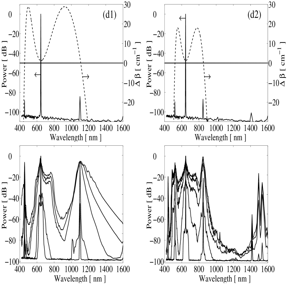
FIG. 1.: Dispersion profiles d1 (left) and d2 (right). Top row: phase mismatch $\Delta\beta$ for direct degenerate FWM (dashed line) and spectrum at $L$=10cm (solid line). Bottom row: spectrum at $L$=20cm, 30cm, 1m, 2m, and 3.7m (down to up).

For a given peak power, the loss and temporal walk-off of the PCF gives the maximum distance $L_{max}$ over which nonlinear processes, and thus the SC generation process, are efficient. From Fig. 1 (left) we see that after the FWM Stokes and anti-Stokes components are generated they broaden in the same way as the central part of the spectrum around the pump. The merging of the spectral parts around $\lambda_{as}$, $\lambda_{p}$, and $\lambda_{s}$ would create an ultra broad spectrum as observed in tapered fibers with high power femtosecond pulses [15, 16]. However, for high power femtosecond pulses the SPM is the dominant mechanism that leads to broadening and merging of the Stokes and anti-Stokes lines with the pump. For low power picosecond pulses the Raman and parametric processes are dominant. Thus, in this particular case, the large frequency shift $\sim\rm{193THz}$ of the degenerate FWM sidebands and the narrow degenerate FWM gain bands $\sim\rm{2THz}$ prevent merging of the pump with the Stokes and anti-Stokes lines to happen within the maximum length $L_{max}$, i.e., before nonlinear effects become negligible. Indeed it is seen from Fig.1, that the spectrum does not change significantly from $\rm{1m}$ to $\rm{3.7m}$. The power transferred to the Stokes and anti-Stokes lines is in effect lost, i.e., the SC process is not very efficient.

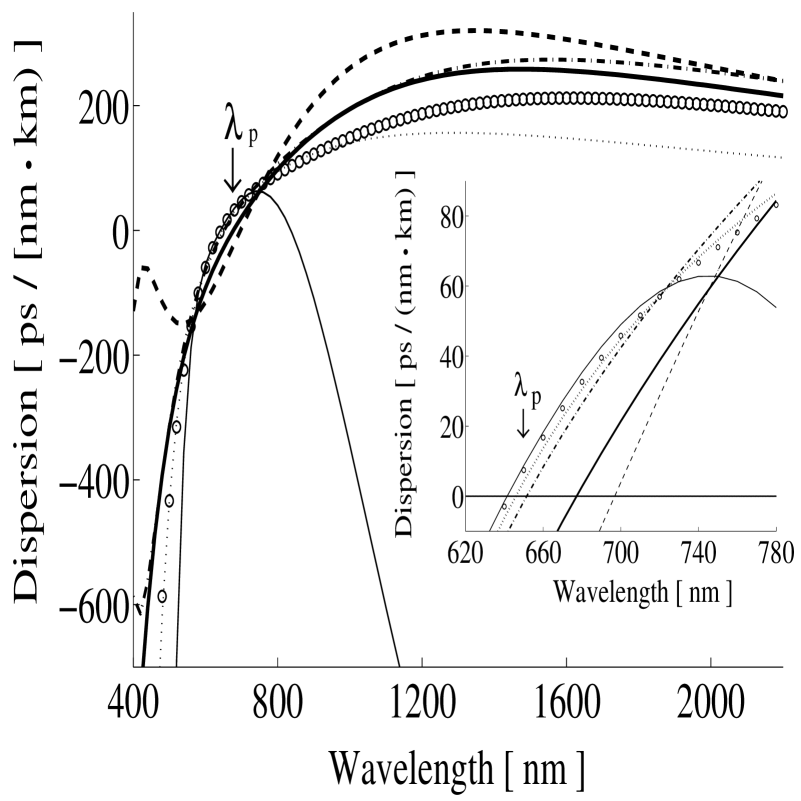
FIG. 2.: Dispersion profile d1 (thick solid line), d2 (dashed line), d3 (dash-dotted line), d4 (dotted line), d5 (circles), and d6 (thin solid line).

By increasing the peak power, it would be possible to achieve merging of the spectral parts around $\lambda_{as}$, $\lambda_{p}$, and $\lambda_{s}$. However, our aim is to keep the low peak power fixed and instead achieve this merging only by engineering the dispersion profile. Thus we modify the dispersion profile to adjust Eq. (6) to be fulfilled for wavelengths $\lambda_{s}$ and $\lambda_{as}$ closer to the pump $\lambda_{p}=\rm{647nm}$. We do so by modifying $\beta_{2}$, $\beta_{4}$, and $\beta_{6}$ as listed in Table I. The phase-matching condition $\Delta\beta=\rm{0}$ then gives $\lambda_{s}=\rm{852nm}$ and $\lambda_{as}=\rm{521nm}$ for case d2-d3. In case d4-d6 additional Stokes and anti-Stokes waves exist. The dispersion profiles and phase-mismatch curves corresponding to the cases in Table I are shown in Fig. 2 and Fig. 3, respectively. It is important to note that the curves $\Delta\beta(\lambda)$ have different slope around $\lambda_{s}$ and $\lambda_{as}$ (see Fig. 3).

We first consider only a shift of the Stokes and anti-Stokes lines closer to the pump and the effect it has on the improvement of the SC generation. Thus, for the dispersion profile d2, the slope of the phase mismatch curve around $\lambda_{s}=\rm{852nm}$ and $\lambda_{as}=\rm{521nm}$ is kept the same as for case d1. It is seen from Fig. 1 (right) that such a shift of the direct degenerate FWM Stokes and anti-Stokes lines closer to the pump is not enough for a complete merging to take place. This can be explained by considering the direct degenerate FWM gain $g(\lambda)$ shown in Fig. 4. The broadening of the Stokes and anti-Stokes lines is strongly influenced by the bandwidth of $g(\lambda)$, which is mainly determined by the slope around $\Delta\beta=0$, i.e., around $\lambda_{s}$ and $\lambda_{as}$. The slope and thus the gain bandwidth is the same in case d1 and d2, which explains why the broadening appears to be unchanged.

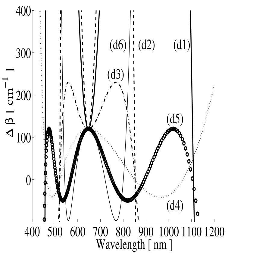
FIG. 3.: Phase mismatch $\Delta\beta(\lambda)$ for dispersion profile d1 (thick solid line), d2 (dashed line), d3 (dash-dotted line), d4 (dotted line), d5 (circles), and d6 (thin solid line).

One way to improve the SC spectrum is to shift the Stokes and anti-Stokes lines even closer to the pump, keeping the slope of the phase mismatch curve around them constant. However, this will not significantly improve the width of the SC spectrum as compared to case d1, because the narrow direct degenerate FWM gain bands will then be in the region, where a SC is already generated by Raman and FWM processes. Moreover, this will lead to even more unusual dispersion profiles than that for case d2 (see Fig. 2), which does not seem to be experimentally realistic.

Instead we fix $\lambda_{s}$ and $\lambda_{as}$ while reducing the slope and thus increasing the gain bandwidth. For dispersion profile d3 the direct degenerate FWM gain bandwidth is thus increased to 16.5THz (see Fig. 4). This leads to broader Stokes and anti-Stokes lines in the initial stages of the SC generation and finally to their merging with the spectrum around the pump as seen from Fig. 5 (right). Thus a SC, which is flat within $\rm{10dB}$ and extending from around 500nm to 900nm is formed after a propagation distance of $L=\rm{2m}$ despite using low-power picosecond pulses. Moreover, the dispersion profile d3 is more realistic, i.e., closer to a real PCF dispersion profile, such as profile d1.

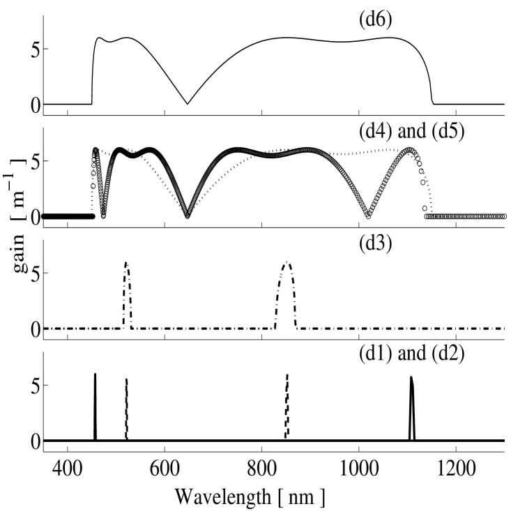
FIG. 4.: Degenerate FWM gain $g(\lambda)$ for dispersion profile d1 (thick solid line), d2 (dashed line), d3 (dash-dotted line), d4 (dotted line), d5 (circles), and d6 (thin solid line).

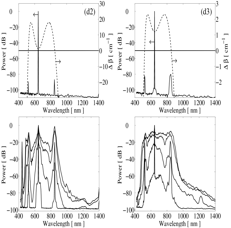
FIG. 5.: Dispersion profiles d2 (left) and d3 (right). Top row: phase mismatch $\Delta\beta$ for direct degenerate FWM (dashed line) and the spectrum at $L=$10cm (solid line). Bottom row: spectrum at $L$=20cm, 30cm, 1m, and 2m (down to up).

The SC process is thus much more efficient with dispersion profile d3 than with d1, since the power in the Stokes and anti-Stokes lines is not lost. However, the SC may be further improved by designing the dispersion such that the phase-mismatch $\Delta\beta(\lambda)$ has two or even three sets of Stokes and anti-Stokes lines, i.e. roots of the polynomium (6). The dispersion profiles d4 and d5 represents such cases with two and three sets of Stokes and anti-Stokes lines, respectively, around which the spectrum can broaden. From the corresponding gain curves in Fig. 4 we see that two gain bands actually overlap and form one broad gain band. The presence of extra Stokes and anti-Stokes lines and the broad gain band could make the SC generation more efficient, provided they do not deplete the pump so much that the central SC spectrum aroud the pump deteriorates.

From Fig. 6 (left) we see that with the dispersion profile d4 the initial stage of the SC generation is indeed improved, the spectrum at $L$=10cm mainly reflecting the gain profile seen in Fig. 4. However, the small dip in the gain curve around 950nm has a strong effect on the evolution of the spectrum, leaving a clear dip at 930nm in the final SC spectrum. Optimizing the position of the two Stokes lines can remove this dip and lead to an even broader SC spectrum than observed in Fig. 5 for one set of Stokes and anti-Stokes lines.

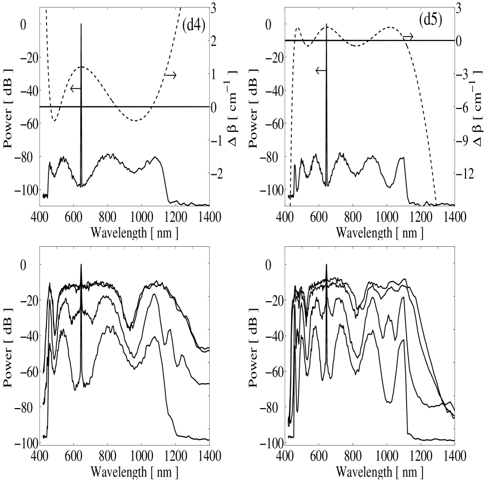
FIG. 6.: Dispersion profiles d4 (left) and d5 (right). Top row: phase mismatch $\Delta\beta$ for direct degenerate FWM (dashed line) and the spectrum at $L$=10cm (solid line). Bottom row: spectrum at $L$=20cm, 30cm, 1m, and 2m (down to up).

Instead we show in Fig. 6 (right) the evolution of the spectrum in a PCF with the dispersion profile d5, which has three sets of Stokes and anti-Stokes lines. The small dip in the gain curve around 800nm (see Fig. 4) is still reflected in the spectrum, but it is now less pronounced and we obtain a final ultra-broad SC spectrum ranging from 450nm to 1250nm within the 20dB level. Of course the dispersion profile may be optimized further to remove the dip and make the SC spectrum more flat and even broader.

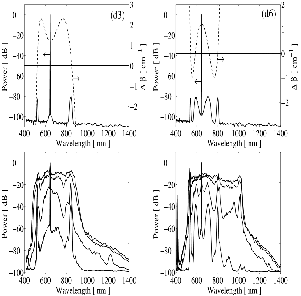
FIG. 7.: Dispersion profiles d3 (left) and d6 (right). Top row: phase mismatch $\Delta\beta$ for direct degenerate FWM (dashed line) and the spectrum at $L$=10cm (solid line). Bottom row: spectrum at $L$=20cm, 30cm, 1m, and 2m (down to up).

So far we have only considered the Stokes and anti-Stokes lines generated directly from the pump through degenerate FWM. However, so-called cascaded FWM processes play also an important role in the evolution of the spectrum, as discussed thoroughly in [6]. In particular, one can use these processes to obtain a broader SC. The dispersion profile d6 is designed to clearly illustrate this effect. It still implies two sets of Stokes and anti-Stokes lines, but now these are very close to the pump, within the regime of wavelengths covered by the central SC generated by the pump. Nevertheless we see in Fig. 7 (right) that additional lines are generated, around which the spectrum broadens, resulting in a final SC spectrum extending from 450nm to 1$\mu$m within 10dB. The line at 1030nm is generated by direct degenerate FWM from the Stokes wave at 720nm, and the line at 1060nm is generated by FWM between the Stokes wave at 720nm and the pump. Thus these cascaded parametric processes result in a spectrum, which is broader than what was obtained with the direct degenerate FWM process in case d3.

Many investigations on designing the dispersion profile in PCFs have been made [11, 12, 13]. In [12] a well-defined procedure to design specific predetermined dispersion profiles is established and it is shown that it is possible to obtain flattened dispersion profiles giving normal, anomalous, and zero dispersion in both the telecommunication window (around 1.55$\mu$m) and the $Ti-Za$ laser wavelength range (around 0.8$\mu$m). This allows us to conclude that the dispersion profiles d3-d5 shown in Fig. 2 could indeed be fabricated. However, it is outside the scope of this work to consider how the specific dispersion profiles may be fabricated.

IV Robustness of SCG to fiber irregularities

The SC generation process that we have considered here is mainly determined by parametric FWM, which requires phase-matching. In the experiments with a PCF with dispersion profile d1 [6, 7] Stokes and anti-Stokes lines due to direct degenerate FWM were generally not observed. This was explained to be due to irregularities along the PCF, leading to violation of the required phase matching condition (6). Thus, in order to conclude that parametric FWM can be used for broad-band SC generation in real PCFs, we check the robustness of the process towards fluctuations of the dispersion coefficients along the fiber.

It has indeed been shown experimentally that a variation of the zero-dispersion wavelength $\lambda_{z}$ of the order of 0.1nm over the entire length of a dispersion shifted fiber could significantly reduce the FWM efficiency [20]. This reduction in the FWM efficiency was later explained theoretically from expressions for the average parametric gain, phase-conjugation efficiency, and gain band-width [21]. It has also been shown that in order to control the dispersion within $\pm$1ps/(km$\cdot$nm), the allowable deviation of the core radius in W-type dispersion-flattened fibers is 0.04$\mu$m, while for other types of dispersion-flattened fibers the allowable core radius deviation is 0.1$\mu$m [22]. As PCFs have an even more complex structure, strong fluctuation of the fiber dispersion could be expected too. However, to our knowledge a thorough study of the influence of fluctuations of the PCF parameters (e.g., core size and pitch) on the variation of the dispersion profile (i.e. the dispersion coefficients $\beta_{2-7}$) is not available.

For a newly developed highly nonlinear PCF with $\lambda_{z}$=1.55$\mu$m, it was recently shown that the variation of $\lambda_{z}$ is only 6nm and the variation of the dispersion slope at $\lambda_{z}$, $D_{z}^{\prime}=dD(\lambda_{z})/d\lambda$, varies between -0.25 and -0.27 ps/(km$\cdot$nm²) over a $150\rm{m}$ span [13]. Expanding the propagation constant to third order around the pump wavelength $\lambda_{p}$=647nm, the dispersion has the form

$$D(\lambda)=-\frac{2\pi c}{\lambda^{2}}\left[\beta_{2}+2\pi c\beta_{3}\left(\frac{1}{\lambda}-\frac{1}{\lambda_{p}}\right)\right].$$ (8)

¿From this expression we find the dispersion coefficients

$$\beta_{2}=\frac{\lambda_{z}^{4}D_{z}^{\prime}}{2\pi c}\left(\frac{1}{\lambda_{p}}-\frac{1}{\lambda_{z}}\right),\quad\beta_{3}=\frac{\lambda_{z}^{4}D_{z}^{\prime}}{4\pi^{2}c^{2}},$$ (9)

which gives the extrema $\beta_{2}^{max}$=7.51ps²/km, $\beta_{2}^{min}=6.83$ps²/km, $\beta_{3}^{max}$=0.44ps³/km, and $\beta_{3}^{min}$=0.40ps³/km and thus the relative variations $\langle\beta_{2}\rangle\simeq\langle\beta_{3}\rangle$=9.5%, where

$$\langle\beta_{k}\rangle\equiv\frac{\beta_{k}^{max}-\beta_{k}^{min}}{(\beta_{k}^{max}+\beta_{k}^{min})/2},\quad\quad k=1,2.$$ (10)

Note that the relative variations of $\beta_{2}$ and $\beta_{3}$ are equal.

We model the effect of a fluctuating dispersion profile by imposing that $\delta\beta$, $\Delta$, and all the dispersion coefficients $\beta_{2-7}$ [see Eq. (4)] vary randomly along the fiber,

$$\delta\beta(z)=\delta\beta+\sigma_{0}(z),\quad\beta_{k,x}(z)=\beta_{k}+\sigma_{k,x}(z),$$ (11)

$$\;\Delta(z)=\;\Delta+\sigma_{1}(z),\quad\beta_{k,y}(z)=\beta_{k}+\sigma_{k,y}(z),$$ (12)

where $k$=2,..,7. The random fluctuation of the coefficients, represented by the $\sigma$-terms, is modelled as Gaussian distributed white noise with zero mean. To achieve the most severe case we use different seeds for all terms. We have thus assumed that the fluctuations affect the dispersion in the two birefringent axis independently. With the results from Ref. [13] in mind we assume that the strength (or variance) of the fluctuations is the same in all coefficients,

$$\frac{\langle\sigma_{0}^{2}(z)\rangle}{\delta\beta}=\frac{\langle\sigma_{1}^{2}(z)\rangle}{\Delta}=\frac{\langle\sigma_{k,x}^{2}(z)\rangle}{\beta_{k}}=\frac{\langle\sigma_{k,y}^{2}(z)\rangle}{\beta_{k}}=\rho,$$ (13)

and use the strength $\rho$=10%.

Random fluctuations of the whole dispersion profile will randomly vary not only the zero-dispersion wavelength $\lambda_{z}$, but more importantly, the phase-mismatch curve $\Delta\beta(\lambda)$, given by Eq. (6). This in turn implies that the FWM gain spectrum $g(\Delta\beta)$, given by Eq. (7), will vary randomly along the fiber, even in the undepleted pump approximation (constant peak power $I_{p}$).

In Fig. 8 we have depicted the fluctuation of the FWM Stokes gain band in the undepleted pump approximation over the first $L$=1mm of a PCF with dispersion profiles d1 ($\lambda_{s}$=1110nm) and d3 ($\lambda_{s}$=852nm). As expected the broader gain band of fiber d3 is reflected in a suppression of the oscillations, as compared to the fiber d1 used in the experiments in [6].

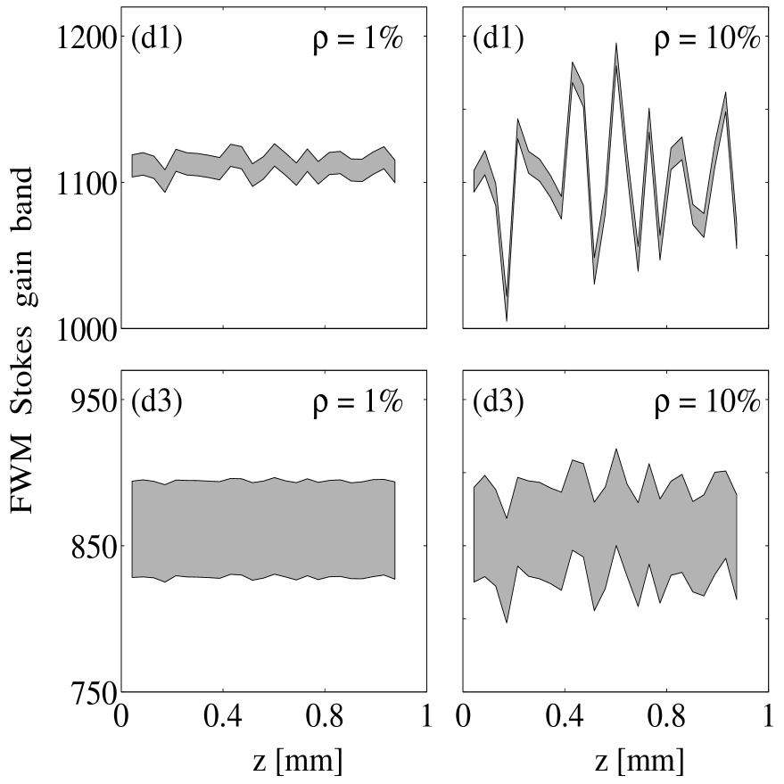
FIG. 8.: Random fluctuations of the FWM Stokes gain band $g(\Delta\beta)$ (grey region), given by Eq. (7), for constant pump $I_{p}$ and $\rho$=1% (left) and $\rho$=10% (right). The upper row is for case d1 and the bottom row for case d2.

The variation of the direct degenerate FWM Stokes gain band gives an impression of the influence of the dispersion fluctuations on the effectiveness of the FWM process. The important factor is the average FWM gain over the fiber length $L$, defined as

$$g_{av}\equiv\frac{1}{L}\int_{0}^{L}g[\Delta\beta(z)]~{}dz,$$ (14)

where we have indicated the $z$-dependence of the phase-mismatch as a result of the fluctuations. In Fig. 9 we show the average FWM Stokes gain calculated over the first $L$=2cm using the undepleted pump approximation. The reduction of the average gain for increasing strength of the fluctuations can be clearly observed.

Theoretically we thus predict that in fiber d1 realistic fluctuations would significantly suppress the Stokes and anti-Stokes lines generated from the pump by direct degenerate FWM, as also stated by Coen et al. [6]. The corresponding simulations, presented in Fig. 10 (left), confirms this prediction. Using direct degenerate FWM to generate an ultra-broad SC in the particular fiber d1 is therefore not realistic.

In contrast, with our proposed fiber d3 with a broad gain band, even fluctuations with $\rho$=10% should not significantly reduce the FWM effectiveness, which is also confirmed by our simulations shown in Fig. 10 (right). In our proposed fibers d4-d5 the FWM gain band is even broader, indicating that fluctuations will have even less impact. Thus our numerical results show that using direct degenerate FWM to generate an ultra-broad SC in really a realistic option.

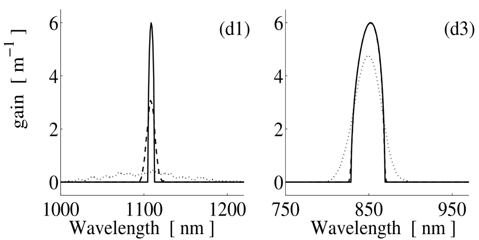
FIG. 9.: Average FWM Stokes gain $g_{av}$ over $L$=2cm, as given by Eq. (14) in the undepleted pump approximation. Shown is case d1 (left) and d3 (right) for $\rho$=0 (solid), $\rho$=1% (dashed), and $\rho$=10% (dotted).

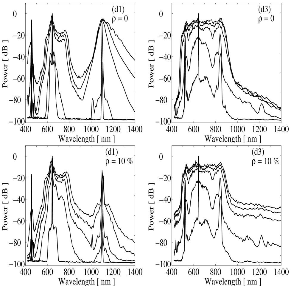
FIG. 10.: Dispersion profiles d1 (left) and d3 (right). Spectrum under influence of fluctuations with strength $\rho$=0 (top row) and $\rho$=10% (bottom row) at $L$=20cm, 30cm, 1m, 2m, and 3.7m (down to up).

V Conclusion

We have numerically investigated SC generation in birefringent PCFs using 30-picosecond pulses with 400-kilowatt peak power. Our results show that by properly designing the dispersion profile and using the generation, broadening, and final merging of widely separated pump and FWM Stokes and anti-Stokes lines the SC generation efficiency can be significantly improved, resulting in a broader SC spectrum and a reduced loss of power to frequencies outside the SC. Thus, by optimising the dispersion profile, we have generated an ultra-broad SC ranging from 450nm to 1250nm within the 20dB level.

We have shown that the key issue is to make sure that the Stokes and anti-Stokes lines are generated close enough to the pump to be able to broaden and merge with the central (pump) part of the SC before nonlinear processes are suppressed due to fiber loss and temporal walk-off. We have also shown that this in turn requires the FWM gain band to be sufficiently broad, which is an essential property of our designed dispersion profiles.

We have finally investigated the robustness of the SC generation process in our proposed fibers towards fluctuations in the parameters along the fiber. Such fluctuation could be detrimental to the phase-sensitive FWM process, which depends on the degree of phase-matching. Simulations including random fluctuations of the dispersion profile along the fiber show that the broad FWM gain band of our proposed fibers improve the robustness and that the process of efficient SC generation survives random fluctuations of a realistic strength.

This work was supported by the Danish Technical Research Council (Grant no. 26-00-0355) and the Graduate School in Nonlinear Science (The Danish Research Agency).

REFERENCES

- [1] R. R. Alfano and S. L. Shapiro, “Emmision in the region 4000 to 7000Åvia four-photon coupling in glass, ” Phys. Rev. Lett. 24, 584-587 (1970).
- [2] R. R. Alfano and S. L. Shapiro, “Observation of self-phase modulation and small-scale filaments in crystals and glasses,” Phys. Rev. Lett. 24, 592-594 (1970).
- [3] The Supercontinuum Laser Source, R. R. Alfano, ed. (Springer-Verlag, New-York, 1989).
- [4] C. Lin and R. H. Stolen, “New nanosecond continuum for excited-state spectroscopy,” Appl. Phys. Lett. 28, 216-218 (1976)
- [5] P. L. Baldeck and R. R. Alfano, “Intensity effects on the stimulated four photon spectra generated by picosecond pulses in optical fibers,” IEEE J.Lightwave Technol. 5, 1712-1715 (1987)
- [6] S. Coen, A. Chao, R. Leonardt, and J. Harvey, J. C. Knight, W. J. Wadsworth, and P. S. J. Russell, “Supercontinuum generation via stimulated Raman scattering and parametric four-wave-mixing in photonic crystal fibers,” J. Opt. Soc. Am. B 26, 753 (2002)
- [7] S. Coen, A. H. L. Chau, R. Leonardt, J. D. Harvey, J. C. Knight, W. J. Wadsworth, and P. S. J. Russell, “White-lightsupercontinuum generation with 60-ps pulse in a photonic crystal fiber,” Opt. Lett. 26, 1356 (2001)
- [8] K. Mori, H. Takara, S. Kawanishi and T. Morioka, “Flatly broadened supercontinuum spectrum generated in a dispersion decreasing fiber with convex dispersion profile,” Electron. Lett. 33, 1806-1808 (1997).
- [9] K. Mori, H. Takara, and S. Kawanishi, “Analysis and design of supercontinuum pulse generation in a single-mode optical fiber,” J. Opt. Soc. Am. B 18, 1780 (2001).
- [10] K. Tamura, H. Kubota, and M. Nakazawa, “Fundamentals of stable continuum generation at high repetition rates,” IEEE J. Quantum Electron. 36, 773-779 (2000).
- [11] A. Ferrando, E. Silvestre, J. J. Miret, and P. Andres, “Nearly zero ultraflattened dispersion in photonic crystal fibers,” Opt. Lett. 25, 790 (2000).
- [12] A. Ferrando, E. Silvestre, P. Andres, J. J. Miret, and M. V. Andres, “Designing the properties of dispersion-flattened photonic crystal fibbers,” Opt. Express 9, 687-697 (2001).
- [13] Kim P. Hansen, Jacob Riis Jensen, Christian Jacobsen, Harald R. Simonsen, Jes Broeng, Peter M. W. Skovgaard, Anders Petersson, Anders Bjarklev, ”Highly Nonlinear Photonic Crystal Fiber with Zero-Dispersion at 1.55 m” OFC ’02 Post Deadline FA 9, 2002
- [14] J. K. Ranka, R. S. Windler, and A. J. Stentz, “ Visible continuum generation in air-silica microstructure optical fibers with anomalous dispersion at 800 nm,” Opt. Lett. 25, 25 (2000).
- [15] T. A. Birks, W. J. Wadsworth, and P. St. J. Russell, “Supercontinuum generation in tapered fibers,” Opt. Lett. 25, 1415 (2000).
- [16] A. V. Gusakov, V. P. Kalosha, and J. Herrmann, “Ultrawide spectral broadening and pulse compression in tapered and photonic fibers,” QELS, pp. 29 (2001).
- [17] J.M. Dudley, L. Provino, N. Grossard, H. Maillotte, R. S. Windler, B. J. Eggeleton and S. Coen, “Supecontinuum generation in air-silica microstructured fibers with nanosecond and femtosecond pulse pumping,” J. Opt. Soc. Am. B 19, 765 (2002)
- [18] C.D. Pole, J.H. Winters and J.A. Nagel, “Dynamical equations for polarization dispersion,” Opt. Lett. 16, 372-374 (1991)
- [19] P.K.A. Wai, C.R. Menyuk and H. H. Chen, “Effects of randomly varying birefringence on soliton interactions in optical fibers,” Opt. Lett. 16, 1735-1737 (1991)
- [20] P. O. Hedekvist, M. Karlsson, and P. A. Andrekson, “Polarization dependence and efficiency in a fiber four-wave mixing phase conjugator with orthogonal pump waves,” Photonics Technol. Lett. 8, 776-778 (1996)
- [21] M. Karlsson, “Four-wave mixing in fibers with randomly varying zero-dispersion wavelength,” J. Opt. Soc. Am. B 15, 2269 (1998)
- [22] N. Kuwaki and M. Ohashi, “Evaluation of longitudinal chromatic dispersion,” J.Lightwave Technol. 8, 1476-1481 (1990)
- [23] J. Garnier and F.Kh. Abdullaev, “Modulational instability by random varying coefficients for the nonlinear Schrö dinger equation,” Physica D 145, 65-83 (2000)
- [24] R. Knapp, “Transmission of solitons through random media,” Physica D 85, 496-508 (1995)
- [25] K.J. Blow, and D. Wood, “Theoretical description of transient stimulated Raman scattering in optical fibers,” IEEE 25, 2665-2673 (1989)
- [26] P. T. Dinda, G. Millot, and S. Wabnitz, “Polarization switching and suppression of stimulated Raman scattering in birefringent optical fibers,” J. Opt. Soc. Am. B 15, 1433 (1998)
- [27] G.P. Agrawal, Nonlinear Fibre Optics, 2nd ed. Academic, San Diego, Calif., (2000).