Resolved diffraction patterns from a reflection grating for atoms

Abstract

We have studied atomic diffraction at normal incidence from an evanescent standing wave with a high resolution using velocity selective Raman transitions. We have observed up to 3 resolved orders of diffraction, which are well accounted for by a scalar diffraction theory. In our experiment the transverse coherence length of the source is greater than the period of the diffraction grating.

Diffraction of atoms by periodic potentials has been a subject of study ever since the beginning of the field of atom optics. The most extensive work has been done in a transmission geometry [1, 2, 3, 4, 5, 6, 7, 8, 9, 10, 11], but reflection gratings have been demonstrated as well. Using evanescent wave mirrors, reflection gratings have been produced by retroreflecting the laser beam creating the evanescent wave [12, 13, 14, 15] or by temporally modulating the intensity of the evanescent wave [16]. Magnetic mirrors have also been rendered periodic by adding an appropriate external magnetic field [17].

Many early experiments on atomic reflection gratings were done at grazing incidence, but this problem proved considerably more subtle than was first imagined (for a review see [18]). It turned out that atomic diffraction at grazing incidence cannot be analogous to the diffraction of light (or X rays) on a reflection grating, because the reflection is not on a hard wall, but on a soft barrier, so that the atom averages out the grating modulation during the bounce. Alternatively, one can show that scalar (i.e. without internal state change) atomic diffraction at grazing incidence on a soft reflection grating would not allow energy and momentum conservation. This is why grazing incidence atomic diffraction must be a process with an internal state change. The change in internal energy allows the process to conserve energy. “Straightforward”, scalar diffraction which is due only to a periodic modulation of the atomic wave front, can only be achieved at normal incidence, as implemented in reference [13].

This experiment suffered however from a resolution which was not quite high enough to separate the individual diffraction peaks. Although it was possible to deconvolve the experimental resolution, and make a quantitative comparison with a scalar diffraction theory, it was disappointing not to be able to directly see the diffraction peaks. Here we discuss an improved version of this experiment in which we use velocity selective Raman transitions to select and analyze a velocity class much narrower than what was possible in the experiments of reference [13]. We are thus able to resolve the diffraction peaks.

Our results are also significant from the point of view of measurements of the roughness of atomic mirrors. These measurements have been performed for both magnetic and evanescent wave mirrors [19, 20, 21, 22, 23]. Some of the interpretation of these measurements relies on theoretical treatments developed in close analogy with the theory of atom diffraction [24], and it is clearly useful to make additional tests of the theory when possible.

Our velocity selection scheme is shown in figure 1. Two counterpropagating, phase-locked lasers induce transitions between the two hyperfine levels of ⁸⁵Rb. They are detuned from resonance by about 600 MHz ($\Delta$ in figure 1). The detuning $\delta$ for this two photon transition depends on the Doppler shift $\delta=k_{\mathrm{L}}(v\pm v_{\rm{R}})$ [25], where $k_{\mathrm{L}}$ is the magnitude of the laser wavevector and $v_{\rm{R}}$ the photon recoil velocity. Thus only atoms with a given velocity $v$ such that $\delta=0$ are resonant. The width of the velocity selection is proportional to $1/\tau$, where $\tau$ is the duration of the pulse. This width can be much smaller than the photon recoil velocity. Figure 1 shows the various laser frequencies used for the Raman transitions and for the evanescent wave atomic mirror.

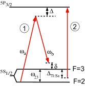
Figure 1: Level diagram for velocity selective Raman transitions and evanescent wave atomic mirror. 1) Frequencies $\omega_{a}$ and $\omega_{b}$ of the two counterpropagating laser beams are separated by ⁸⁵Rb hyperfine frequency $\omega_{23}$ plus Raman detuning $\delta$. 2) The Ti:Sa laser that creates the evanescent wave mirror is blue detuned for atoms in $F=3$ and red detuned for atoms in $F=2$, thus only atoms in $F=3$ bounce on the atomic mirror.

Our experiment follows closely the procedures of reference [23]. It consists of two distinct sequences, each using two Raman pulses. First, to measure the atomic velocity distribution after reflection, the following sequence is used. A sample of ⁸⁵Rb atoms are optically pumped into F=2 after preparation in a magneto-optical trap and optical molasses, and released at time $t=0$. A constant magnetic field of 750 mG is turned on, to define the axis of quantization and split the $m_{F}$ levels. A Raman $\pi$-pulse is applied at $t=8$ ms with detuning $\delta_{S}$ (selection). This transfers atoms from $|2,0,\delta_{S}/k_{\mathrm{L}}-v_{\rm{R}}\rangle$ into $|3,0,\delta_{S}/k_{\mathrm{L}}+v_{\rm{R}}\rangle$. At $t=47$ ms, the Ti:Sa laser that forms the evanescent wave is turned on. Its detuning is chosen so that it reflects atoms in F=3 (blue detuning), while being attractive for the state F=2 (red detuning). This eliminates unselected atoms left in F=2. The Ti:Sa laser is turned off at $t=67$ ms. At $t=120$ ms, a second $\pi$-pulse is applied, with detuning $\delta_{A}$ (analysis), returning atoms in $|3,0,\delta_{A}/k_{\mathrm{L}}+v_{\rm{R}}\rangle$ to $|2,0,\delta_{A}/k_{\mathrm{L}}-v_{\rm{R}}\rangle$. At $t=124$ ms we switch on a pushing beam for 2 ms, resonant for F=3, which accelerates F=3 atoms away from the detection region. Finally, the measured signal is the fluorescence of the remaining atoms in F=2, illuminated by a resonant probe beam with repumper and measured with a photomultiplier tube. To measure the number of atoms at the end of the sequence, we evaluate the area of a Gaussian fit of the fluorescence signal.

This first sequence is repeated fixing $\delta_{S}$ and scanning $\delta_{A}$. In this way, we build up the velocity distribution of the reflected atoms. The frequencies $\delta_{A}$ are selected in a random order, and after each shot, a second shot is taken with $\delta_{S}=\delta_{B}$ (background) sufficiently detuned so that it does not transfer any atoms. Since we detect all atoms in F=2, there is a small background of atoms that have not been selected, but instead scattered a photon, thereby finishing in the same state as the atoms that have been selected. This can occur during the analysis pulse, and during interaction with the Ti:Sa laser. We estimate that around $10\%$ of atoms undergo such processes in the evanescent wave, and $1\%$ during each $\pi$ pulse. Most of these atoms are accounted for by the background shot. The background shot is subtracted from the signal shot, and the difference is the data point. We average each data point 5 times, so that a diffraction pattern takes around 20 minutes to acquire.

To complete the experiment, we need to know the velocity distribution of the atoms selected by the first pulse. To measure this we employ a second sequence, essentially the same as the first, but without the mirror. Atoms are prepared in $F=3$ at the end of the optical molasses. At $t=8\,\mbox{ms}$ the first Raman pulse transfers resonant atoms to $F=2$, other atoms are removed with the pushing beam. At $t=22\,\mbox{ms}$ the second Raman pulse transfers atoms back in $F=3$ and we finally detect only atoms in $F=3$. By scanning the detuning of the second Raman pulse we can measure the velocity width of the atoms selected by the first pulse. The observed velocity distribution is well fitted by a Gaussian function with a width given by $2\,k_{\mathrm{L}}\,\sigma_{v}\approx 2\pi/\tau$. Because of the convolution of the selection and analysis pulses, the observed velocity distribution is approximately $\sqrt{2}$ times larger than that due to the selection pulse alone. For a pulse length of $\tau=120$ $\mu$s, the measured rms width is $2\,k_{\mathrm{L}}\,\sigma_{v}=2\pi\times 7.7$ kHz or $\sigma_{v}=0.50\,v_{\rm{R}}=3.0$ mm.s^-1. We will use this Gaussian function as our resolution function $S(\delta)$. Any differences between the two measured velocity distributions are attributed to the action of the diffraction grating.

The reflection grating for atoms is made by retroreflecting a small proportion of light that makes the evanescent wave: a standing wave is created on the mirror and the potential seen by the atoms can be written (neglecting the van der Waals interaction for the moment)

$$U(x,z)=U_{0}e^{-2\,\kappa\,z}(1+\epsilon\cos(2\,k_{x}\,x)),$$ (1)

where $\epsilon$ is the contrast of the interference pattern, $1/\kappa$ is the decay length of the electric field, and $k_{x}$ is the propagation wave vector of the evanescent wave. The contrast $\epsilon$ can be written:

$$\epsilon=\frac{2\sqrt{R}}{1+R}\frac{k_{x}^{2}-\kappa^{2}}{k_{x}^{2}+\kappa^{2}},$$ (2)

where $R=I_{R}/I_{0}$ is the intensity fraction of the laser beam that is retroreflected. To a good approximation, the grating behaves as a thin phase grating, producing a modulated de Broglie wave whose predicted phase modulation index is:

$$\varphi=\frac{2\pi}{\lambda_{\rm{dB}}}\frac{\epsilon}{\kappa},$$ (3)

where $\lambda_{\rm{dB}}$ is the de Broglie wavelength of the atomic cloud incident on the mirror. The van der Waals force introduces a multiplicative correction that here increases the phase modulation index $\varphi$ [13] by 12% .

In our experiments, $\kappa=1.14\,k_{\rm{L}}$. When the contrast of the grating $\epsilon$ is of order $\lambda_{\rm{dB}}/\lambda_{\rm{L}}$, we have $\varphi\sim 1$ rad, and the diffraction is efficient. Here, $\lambda_{\rm{dB}}=7$ nm and $\lambda_{\rm{L}}=780$ nm. Thus we only need a very weak contrast $\epsilon\sim 10^{-2}$, corresponding to $R\sim 10^{-4}$.

The $n$th diffraction order acquires a transverse momentum of $2\,n\,\hbar\,k_{x}$ and has an intensity of $J_{n}^{2}(\varphi)$, where $J_{n}$ is the Bessel function of order $n$. Here, $k_{x}=1.5\,k_{\rm{L}}$, so to distinguish two successive diffraction orders, we must have a velocity selection in the $x$ direction better than $1.5\,v_{\rm{R}}$.

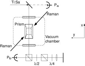
Figure 2: Experimental geometry. The Ti:Sa strikes the prism from below, with an angle of incidence $\theta=53^{\circ}$. The system of polarizers and wave plates allows us to reflect a small controlled amount of the Ti:Sa beam.

Figure 2 shows the experimental geometry. The mirror is 20.7 mm below the magneto-optical trap. It is a prism with an index of refraction of $n=1.869$ and the angle of incidence of the Ti:Sa laser $\theta=53^{\circ}$. The prism is superpolished and has a roughness of about $0.07$ nm deduced from measurements made with an atomic force microscope and a Zygo optical heterodyne profiler. To remove the degeneracy of the Zeeman sublevels, a magnetic bias field of 750 mG is applied along the direction of propagation of the Raman beams. After the first $\pi$ pulse, the direction of the magnetic bias field is rotated by $45^{\circ}$ so that it lies along the $y$-direction, corresponding to the quantization axis of the evanescent wave. The change is carried out over 10 ms, so that the atoms adiabatically follow the field. The direction of the field is turned back after the bounce for the second $\pi$ pulse.

Also shown in figure 2 is the setup for measuring and controlling the retroreflected power $R$. The two wave plates control the power, the half wave plate is used as a coarse and the quarter wave plate as a fine adjustment. A cat’s eye arrangement is used to control the spatial superposition and size of the return beam. The experimental setup for the Raman beams has been described elsewhere [23].

To measure $R$, first the incident power is found from $P_{a}$ and the (known) transmission $T$ of the first mirror in figure 2. Then the quarter wave plate is turned to the position that maximizes the power $P_{b}$. Next, the position of the half wave plate is fixed so that $P_{b}/(P_{a}/T)$ is the maximum value of $R$ desired. Finally, the quarter wave plate is adjusted to vary the $R$ over the desired range. The fraction of power reflected $R$ is then deduced from the relationship

$$R=\frac{P_{b}^{\mathrm{max}}}{P_{a}/T}\frac{\left(P_{b}^{\mathrm{max}}-P_{b}\right)}{P_{b}^{\mathrm{max}}}.$$ (4)

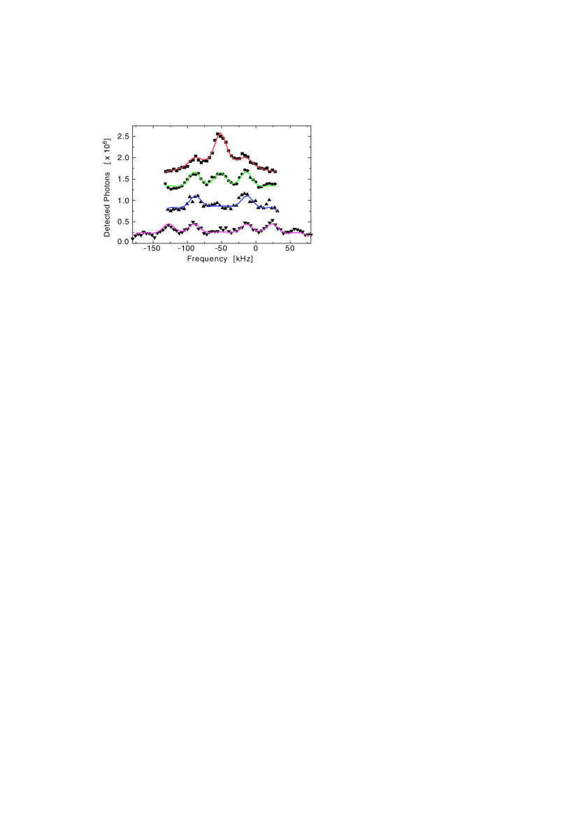
Figure 3: Velocity profile of diffracted atoms (curves have been offset for display purposes). The amplitude of the diffraction grating is increased from top to bottom ($R=2.8\times 10^{-5}$, $5.7\times 10^{-5}$, $1.7\times 10^{-4}$, $1.5\times 10^{-3}$). We can observe up to 3 separated orders of diffraction.

Figure 3 (a,b,c,d) presents the atomic experimental velocity distribution after reflection when $R=2.8\times 10^{-5}$, $5.7\times 10^{-5}$, $1.7\times 10^{-4}$, $1.5\times 10^{-3}$ of the incident laser intensity is retroreflected, for $\Delta_{Ti:Sa}=2.5$ GHz. The diffraction orders are more and more populated when the intensity of the retroreflected beam increases, and the different diffraction orders are well resolved. The expected separation between successive orders of diffraction is $4(\cos\alpha)\,k_{x}\,v_{\rm{R}}=2\pi\times 33$ kHz, where $\alpha=43^{\circ}$ is the measured angle between the Raman beams and the evanescent wave propagation direction. The data in the figure give a peak separation of $\delta_{0}=2\pi\times 38$ kHz. The difference between the calculated and observed peak separations is rather large, but we currently have no satisfactory explanation for this discrepancy.

The data are fitted by the following function:

$$a+b\,\mathrm{R}(\delta)\times\sum_{n}\left[J_{n}^{2}(\phi)\,\delta(\delta-n\,\delta_{0})\ast\left\{\mathrm{S}(\delta)+c\,\mathrm{M}(\delta)\right\}\right]$$ (5)

Each diffraction order has a weight given by the value of the Bessel function $J_{n}^{2}(\phi)$ and is convolved by the resolution function $\mathrm{S}(\delta)$, plus the function $\mathrm{M}(\delta)$ that accounts for a background of atoms whose velocity distribution is imposed by the spatial extent of the mirror. The resolution function is a gaussian profile with rms width 7.7 kHz. This entire function is then multiplied by the function $\mathrm{R}(\delta)$ which takes account of the spatial variation of the Raman beams.

The widths of the functions $\mathrm{R}$, $\mathrm{S}$ and $\mathrm{M}$ are calculated from measured values, so that there are only four adjustable parameters for the fitting procedure: an offset $a$, the amplitude of the curve $b$, the phase modulation index $\phi$, and the background term $c$.

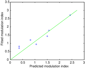
Figure 4: Fitted and predicted phase modulation index. The fitted values are deduced from the velocity profile of the diffracted atoms and the predicted ones are calculated from the measurement of the amount of reflected power $R$ (taking into account the Van der Waals interaction). The straight line fit has gradient 1.11(8).

Figure 4 shows the fitted and predicted phase modulation indices. The two are in satisfactory agreement to within our uncertainty, which is chiefly limited by the uncertainty in the superposition of the return beam.

To conclude, the fact that the peak heights can be accounted for by a series of Bessel functions depending on a single parameter, the modulation index, is quite remarkable and constitutes the central result of this work. It shows that one can reach a regime in which the atomic diffraction on a corrugated mirror can be described simply as a reflection of a scalar matter wave, with a phase modulation of the reflected wavefront calculated within the straightforward thin phase grating approximation [26]. In this regime, one thus have a close analogy to light diffraction off a reflection grating.

This work was supported by the European Union under grants IST–1999–11055 and HPRN–CT–2000–00125, and by the DGA grant 00.34.025.

References

- [1] Gould P L, Ruff G A, and Pritchard D E 1986 Phys. Rev. Lett. 56 827
- [2] Martin P J, Gould P L, Oldaker B G, Miklich A H, and Pritchard D E 1987 Phys. Rev. A 36 2495
- [3] Martin P J, Oldaker B G, Miklich A H, and Pritchard D E 1988 Phys. Rev. Lett. 60 515
- [4] Gould P L, Martin P J, Ruff G A, Stoner R E, Picque J–L, and Pritchard D E 1991 Phys. Rev. A 43 585
- [5] Chapman M S, Ekstrom C R, Hammond T D, Schmiedmayer J, Tannian B E, Wehinger S, and Pritchard D E 1995 Phys. Rev. A 51 R14
- [6] Giltner D M, McGowan R W, and Lee S A, 1995 Phys. Rev. Lett. 75 2638
- [7] Kunze S, Durr S, and Rempe G 1996 Europhys. Lett. 34 343
- [8] Kunze S, Dieckmann K, and Rempe G 1997 Phys. Rev. Lett. 78 2038
- [9] Bernet S, Oberthaler M, Abfalterer R, Schmiedmayer J, and Zeilinger A 1996 Phys. Rev. Lett. 77 5160
- [10] Kozuma M, Deng L, Hagley E W, Wen J, Lutwak R, Helmerson K, Rolston S L, and Philips W D 1999 Phys. Rev. Lett. 82 871
- [11] Kokorowski D A, Cronin A D, Roberts T D, and Pritchard D E 2001 Phys. Rev. Lett. 86 2191
- [12] Brouri R, Asimov R, Gorlicki M, Feron S, Reinhardt J, Lorent V, and Haberland H 1996 Opt. Comm. 124 448
- [13] Landragin A, Cognet L, Horvath G Z K, Westbrook C I, and Aspect A 1997 Europhys. Lett. 39 485
- [14] Cognet L, Savalli V, Horvath G Z K, Holleville D, Marani R, Westbrook N, Westbrook C I, and Aspect A 1998 Phys. Rev. Lett. 81 5044
- [15] Christ M, Scholz A, Schiffer M, Deutchmann R, and Ertmer W 1994 Opt. Comm. 107 211
- [16] Steane A, Szriftgiser P, Desbiolles P, and Dalibard J 1995 Phys. Rev. Lett. 74 4972
- [17] Rosenbusch P, Hall B V, Hughes I G, Saba C V, and Hinds E A 2000 Phys. Rev. A 61 031404
- [18] Henkel C, Wallis H, Westbrook N, Westbrook C, Aspect A, Sengstock K, and Ertmer W 1999 Appl. Phys. B 69 277
- [19] Landragin A, Labeyrie G, Henkel C, Kaiser R, Vansteenkiste N, Westbrook C I, and Aspect A 1996 Opt. Lett. 21 1591
- [20] Voigt D, Wolschrijn B T, Jansen R, Bhattacharya N, Spreeuw R J C, and van Linden van den Heuvell H B 2000 Phys. Rev. A 61 063412
- [21] Saba C V, Barton P A, Boshier M G, Hughes I G, Rosenbusch P, Sauer B E, and Hinds E A 1999 Phys. Rev. Lett. 82 468
- [22] Cognet L, Savalli V, Featonby P D, Helmerson K, Westbrook N, Westbrook C I, Phillips W D, Aspect A, Zabow G, Drndic M, Lee C S, Westervelt R M, and Prentiss M 1999 Europhys. Lett. 47 538
- [23] Savalli V, Stevens D, Estève J, Featonby P D, Josse V, Westbrook N, Westbrook C I, and Aspect A 2002 Phys. Rev. Lett. 88 250404
- [24] Henkel C, Moelmer K, Kaiser R, Vansteenkiste N, Westbrook C, and Aspect A 1997 Phys. Rev. A 55 1160
- [25] Kasevich M, Weiss D, Riis E, Moler K, Kasapi S, and Chu S 1991 Phys. Rev. Lett. 66 2297
- [26] Henkel C, Courtois J Y, and Aspect A 1994 J. Phys. II France 4 1955