Transient growth in Taylor-Couette flow

Abstract

Transient growth due to non-normality is investigated for the Taylor-Couette problem with counter-rotating cylinders as a function of aspect ratio $\eta$ and Reynolds number $Re.$ For all $Re\leq 500$, transient growth is enhanced by curvature, i.e. is greater for $\eta<1$ than for $\eta=1$, the plane Couette limit. For fixed $Re<130$ it is found that the greatest transient growth is achieved for $\eta$ between the Taylor-Couette linear stability boundary, if it exists, and one, while for $Re>130$ the greatest transient growth is achieved for $\eta$ on the linear stability boundary. Transient growth is shown to be approximately 20% higher near the linear stability boundary at $Re=310$, $\eta=0.986$ than at $Re=310$, $\eta=1$, near the threshold observed for transition in plane Couette flow. The energy in the optimal inputs is primarily meridional; that in the optimal outputs is primarily azimuthal. Pseudospectra are calculated for two contrasting cases. For large curvature, $\eta=0.5$, the pseudospectra adhere more closely to the spectrum than in a narrow gap case, $\eta=0.99$.

Keywords: Taylor-Couette instability, transition to turbulence

I Introduction

Two shear-driven flows bear the name of Couette: the flow between differentially rotating concentric cylinders is called cylindrical Couette flow, or more commonly, Taylor-Couette flow, while the flow between infinite parallel plates translating at different velocities while maintaining a constant separation is called plane Couette flow. Exact solutions, both called Couette solutions, to the Navier-Stokes equations for each of these configurations are easily calculated and serve as illustrations in most textbooks. Each of these two flows has become a paradigm of hydrodynamic stability theory.

Taylor-Couette flow can be considered to be a paradigm of understanding. In 1923, Taylor Taylor carried out calculations of the linear instability of Couette flow to the onset of axisymmetric vortices and compared these with experiment, obtaining agreement which remains remarkable even by today’s standards. In later research, increasingly ornate and beautiful experimental patterns were discovered, e.g. Coles ; Andereck ; Taggribbons , and correspondingly elaborate numerical, asymptotic, and theoretical calculations, e.g. Krueger ; Marcus ; Langford , reproduced and explained these patterns, again with remarkable accuracy; see Swinney ; DrazinReid ; Taggreview ; ChossatIooss .

Plane Couette flow, on the other hand, can be considered to be a paradigm of mystery. For plane parallel flows, Squire’s theorem Squire firmly establishes that the linear instability with the lowest critical Reynolds number is spanwise invariant. Armed with this theorem, researchers have long known, and more recently proved Romanov , that plane Couette flow is linearly stable at all Reynolds numbers. Yet, in laboratory experiments Tillmark and in numerical simulations Lundbladh , plane Couette flow undergoes sudden transition to three-dimensional turbulence. Since at least the 1960’s researchers have explored various mechanisms for transition in plane Couette flow which bypass linear instability and Squire’s theorem. An element shared by all of these approaches, independent of the theoretical mechanism proposed for instability, is the presence of streamwise vortices Joseph ; Butler ; Trefethen_93 ; Reddygrowth ; Waleffe , i.e. perturbations which, unlike those deemed critical by Squire’s theorem, are not spanwise invariant, but are instead invariant or almost invariant in the streamwise direction. These are analogous to the Taylor vortices which, in Taylor-Couette flow, are the eigenvectors responsible for the linear instability and are realized in experiments and in nonlinear numerical simulations.

One major line of research has focused on the effect of the non-normality of the operator governing the linear stability of plane Couette flow Butler ; Trefethen_93 ; Reddygrowth . Such operators may lead to transient growth dynamics, even in the absence of linear instability, allowing nonlinear effects to take over before the final exponential decay exhibited by the linear evolution. Plane Couette flow can exhibit transient growth of several orders of magnitude; the initial conditions which maximize the transient growth, called optimal perturbations, contain streamwise vortices. Transient growth is closely associated with the sensitivity of the spectrum to small perturbations of the operator, quantified by the pseudospectra Trefethen_93 .

The concepts of pseudospectra, non-normality, transient growth, and optimal perturbations, have been rarely applied to Taylor-Couette flow Gebhardt ; Meseguer , probably because conventional linear stability analysis is so successful in explaining the transitions observed. However, the large parameter space of Taylor-Couette flow offers the possibility of tuning the system from a normal operator, which does not support any transient growth, to a highly non-normal operator. Because of translational and Galilean invariance, plane Couette flow depends only on the distance $2d$ between the plates, the relative velocity $2\Delta U$ of the plates, and the kinematic viscosity $\nu$, which are combined into a single nondimensional parameter, the Reynolds number defined conventionally as $Re\equiv\Delta Ud/\nu$. In contrast, because of curvature effects in Taylor-Couette flow, both the inner and outer radii $r_{\rm in}$ and $r_{\rm out}$ (or gapwidth $2d=r_{\rm out}-r_{\rm in}$ and average radius $\bar{r}=(r_{\rm in}+r_{\rm out})/2$) play a role. Because transformation to a rotating reference frame would introduce a Coriolis term into the equations, the flow depends on the angular velocities of both the inner and the outer cylinders, $\Omega_{\rm in}$ and $\Omega_{\rm out}$. The five dimensional parameters can be combined into three non-dimensional parameters in various ways. Our choice is $\eta\equiv r_{\rm in}/r_{\rm out}$, $\mu\equiv\Omega_{\rm out}/\Omega_{\rm in}$, and $Re\equiv r_{\rm in}\Omega_{\rm in}d/\nu$.

The idea of trying to approach the stability of plane Couette flow via Taylor-Couette flow is an appealing one and has inspired a number of investigations. The axisymmetric Taylor-vortex solution undergoes a secondary bifurcation to a non-axisymmetric wavy-vortex solution Coles ; Marcus . In a search for states intermediate in complexity between the Couette solution and turbulent plane Couette flow, Nagata Nagata90 ; Nagata98 took the limits of a narrow gap and almost corotating cylinders and discovered that, while the Taylor-vortex solution ceases to exist as the Coriolis term (i.e. the average angular velocity) is decreased, the wavy-vortex solution could be continued to the plane Couette limit. Faisst & Eckhardt Eckhardt showed that these wavy solutions also exist for counter-rotating cylinders and that the lowest Reynolds number at which they first appear (via a saddle-node bifurcation) becomes independent of the rotation ratio as $\eta\rightarrow 1$. Finally, Prigent and Dauchot Prigent have discovered that an analog of the spiral turbulence state of Taylor-Couette flow also exists for plane Couette flow.

Our investigation goes somewhat in the opposite direction. While the investigations cited above considered steady or traveling states known to exist in Taylor-Couette flow and continued them to the plane Couette limit, we take the ideas of pseudospectra, non-normality, transient growth, and optimal perturbations, apply them to Taylor-Couette flow and investigate the limit as Taylor-Couette flow approaches plane Couette flow. We focus on a given representative azimuthal and axial wavenumber and explore the stability characteristics of counter-rotating Taylor-Couette flow for a range of Reynolds numbers and radius ratios. In a related study, Meseguer Meseguer studied transient effects – optimized over azimuthal and axial wavenumbers – for a specified radius ratio and varying Reynolds number and angular velocity ratio. Since Taylor-Couette flow is linearly stable for $\Omega_{\rm in}=0$, Meseguer suggests that transient growth plays an important role in the transition to turbulence observed experimentally Coles for $\Omega_{\rm in}=0$, $-\Omega_{\rm out}\gg 1$, a theory contested by Gebhardt & Grossman Gebhardt .

Why calculate transient growth in Taylor-Couette flow, one of the major success stories of linear stability theory? Transient growth is a new tool in linear stability theory, whose worth and longevity have yet to be proved. It has up to now been applied to flows in which transition from the basic laminar state is not understood. It is therefore worthwhile to calculate transient growth in Taylor-Couette flow, in which transition is believed to be completely understood by hydrodynamicists. This could provide information about the value and significance of transient growth calculations. The other side of the coin is that the paradigmatic status of Taylor-Couette flow should be maintained. As new tools or measurements become available, they should be brought to bear on this basic flow in order for hydrodynamicists to extract additional knowledge about Taylor-Couette flow.

II Governing Equations and Numerical Methods

II.1 Taylor-Couette flow

The Couette solution is the unique solution of the form $\underline{U}=U_{\mbox{\tiny}C}(r)\underline{e}_{\theta}$ to the incompressible Navier-Stokes equations:

$$\frac{\partial\underline{U}}{\partial t}+(\underline{U}\cdot\nabla)\underline{U} = -\nabla P+\frac{1}{Re}\Delta\underline{U},$$ (1a)

$$\nabla\cdot\underline{U} = 0,$$ (1b)

$$\underline{U}(r=\bar{r}-1)=1, \underline{U}(r=\bar{r}+1)=\frac{\mu}{\eta}.$$ (1c)

Distances have been nondimensionalized by $(r_{\rm out}-r_{\rm in})/2$ and velocities by $r_{\rm in}\Omega_{\rm in}$. We recall that

$$\eta\equiv r_{\rm in}/r_{\rm out},\quad\mu\equiv\Omega_{\rm out}/\Omega_{\rm in},\quad Re=r_{\rm in}\Omega_{\rm in}(r_{\rm out}-r_{\rm in})/(2\nu)$$ (2)

where $r_{\rm in}$, $r_{\rm out}$, $\Omega_{\rm in}$, $\Omega_{\rm out}$ are the inner and outer cylindrical radii and angular velocities, respectively, and $\nu$ is the kinematic viscosity. Definition (2) of $Re$, chosen for compatibility with the plane Couette convention for the case $\mu=-1$, differs by a factor of two from the conventional definition employed in Taylor-Couette flow. The average radius is $\bar{r}=(1+\eta)/(1-\eta)$. Thus, the limit $\eta\rightarrow 1$ corresponds to $\bar{r}\rightarrow\infty$; we refer to either of these limits as convenient.

The Couette solution is:

$$U_{\mbox{\tiny}C}(r) = Ar+\frac{B}{r},$$ (3a)

$$A=\frac{\mu-\eta^{2}}{2\eta(1+\eta)}, B=\frac{2\eta(1-\mu)}{(1-\eta)(1-\eta^{2})}.$$ (3b)

The expressions for $A$ and $B$ again differ from the standard ones by factors of two due to our use of $(r_{\rm out}-r_{\rm in})/2$ as unit of length. Expression (3) can be viewed as a superposition of solid body rotation, $Ar$, and the flow due to a point vortex, $B/r$. As $\eta\rightarrow 1$, the leading terms of these two contributions become equal and opposite: $Ar\sim-B/r\sim(\mu-1)\bar{r}/4$. For $\eta\sim 1$, we therefore rewrite (3) in the following equivalent form not subject to this cancellation error:

$$U_{\mbox{\tiny}C}(r)=\frac{1}{4r\bar{r}(\bar{r}-1)}\;\left[2\bar{r}^{3}\;((\mu+1)+(\mu-1)y)\right.+\bar{r}^{2}\;(3(\mu-1)+4(\mu+1)y+(\mu-1)y^{2})$$

$$+\left.2\bar{r}y\;((\mu-1)+(\mu+1)y)-(\mu-1)(1-y^{2})\right]$$ (4)

where

$$y\equiv r-\bar{r}.$$ (5)

The equations we consider are the Navier-Stokes equations (1) linearized about the Couette solution (3) or (4):

$$\frac{\partial u_{r}}{\partial t}+\frac{U_{\mbox{\tiny}C}}{r}\frac{\partial u_{r}}{\partial\theta}-\frac{2U_{\mbox{\tiny}C}}{r}u_{\theta}=-\frac{\partial p}{\partial r}+\frac{1}{Re}\Big{(}\Delta u_{r}-\frac{u_{r}}{r^{2}}-\frac{2}{r^{2}}\frac{\partial u_{\theta}}{\partial\theta}\Big{)},$$ (6a)

$$\frac{\partial u_{\theta}}{\partial t}+\frac{U_{\mbox{\tiny}C}}{r}\frac{\partial u_{\theta}}{\partial\theta}+\frac{U_{\mbox{\tiny}C}}{r}u_{r}+{U_{\mbox{\tiny}C}}^{{}^{\prime}}u_{r}=-\frac{1}{r}\frac{\partial p}{\partial\theta}+\frac{1}{Re}\Big{(}\Delta u_{\theta}-\frac{u_{\theta}}{r^{2}}+\frac{2}{r^{2}}\frac{\partial u_{r}}{\partial\theta}\Big{)},$$ (6b)

$$\frac{\partial u_{z}}{\partial t}+\frac{U_{\mbox{\tiny}C}}{r}\frac{\partial u_{z}}{\partial\theta}=-\frac{\partial p}{\partial z}+\frac{1}{Re}\Big{(}\Delta u_{z}\Big{)},$$ (6c)

$$\frac{\partial u_{r}}{\partial r}+\frac{1}{r}u_{r}+\frac{1}{r}\frac{\partial u_{\theta}}{\partial\theta}+\frac{\partial u_{z}}{\partial z}=0,$$ (6d)

subject to the boundary conditions

$$u_{r}=u_{\theta}=u_{z}=0\quad{\rm at}\quad r=\bar{r}\pm 1$$ (6e)

with

$$\Delta=\frac{\partial^{2}}{\partial r^{2}}+\frac{1}{r}\frac{\partial}{\partial r}+\frac{1}{r^{2}}\frac{\partial^{2}}{\partial\theta^{2}}+\frac{\partial^{2}}{\partial z^{2}}.$$

The Taylor-Couette geometry and the Couette solution are homogeneous in the azimuthal ($\theta$) and axial ($z$) direction, which are analogous to the streamwise ($x$) and spanwise ($z$) directions in plane Couette flow. Table 1 summarizes the equivalence of the coordinate systems for plane Couette and Taylor-Couette flow. Solutions to (6e) which are spatially bounded are therefore trigonometric in each of these directions, with wavenumbers $m$ and $\beta,$

$$(u_{r},u_{\theta},u_{z},p)=(\hat{u}_{r},\hat{u}_{\theta},\hat{u}_{z},\hat{p})(r,t)\exp(im\theta+i\beta z).$$ (6)

The parameter space is too vast to permit full exploration. In this study, we limit ourselves to $\mu=-1$, $m=0$, and $\beta=\pi/2$. We choose $\mu=-1$ so that the average angular velocity vanishes.

The choice $m=0$ of axisymmetric perturbations is made for simplicity. In plane Couette flow, the transient growth achieved by streamwise-independent perturbations is, while not maximal, very close to the optimal value. Although the study of transient growth in Taylor-Couette flow is relatively unexplored, its linear instability has been extensively studied, e.g. Taylor ; Krueger ; Langford ; DrazinReid ; Gebhardt . The linear instability undergone by Taylor-Couette flow with counter-rotating cylinders is usually non-axisymmetric and leads to spirals rather than vortices. However, the threshold associated with axisymmetric perturbations is very close to the actual non-axisymmetric threshold. Indeed, the thresholds are so close that the instability was thought to be axisymmetric until 1966, when calculations by Krueger, Gross and DiPrima Krueger confirmed experimentally by Coles Coles showed the first instability to be non-axisymmetric for $\mu$ sufficiently negative, more precisely $\mu\lesssim 0.78$ in the narrow-gap limit. Note that the correspondence between the streamwise wavenumber $\alpha$ of plane Couette flow and the azimuthal wavenumber $m$ of Taylor-Couette flow is $m\sim\bar{r}\alpha$, since $x\sim r\theta$. Setting $m$ to correspond to a fixed non-zero value of $\alpha$ would thus require increasing $m$ through integer values as $\eta\rightarrow 1$ or $\bar{r}\rightarrow\infty$.

The choice $\beta=\pi/2$ corresponds to an axial wavelength of 4. Since our choice of length scales dictates that the radial gap is of width 2, this means that a single vortex has the same axial as radial extent, i.e. is approximately circular. The axial wavelength corresponding to linear instability is somewhat smaller than this for counter-rotating cylinders by as much as 20%, but is nonetheless close.

We eliminate $\hat{u}_{z}$ and $\hat{p}$ by using (6c) and the condition of incompressibility (6d), obtaining evolution equations in $\underline{u}=(\hat{u}_{r},\hat{u}_{\theta})$. The perturbations $(\hat{u}_{r},\hat{u}_{\theta})$ are represented as series of Chebyshev polynomials in $y\equiv r-\bar{r}$, which are evaluated at the Gauss-Lobatto points Canuto .

The evolution equation is written symbolically for the state vector $\underline{u}=(\hat{u}_{r},\hat{u}_{\theta})^{T}$ as

$$\frac{\partial}{\partial t}\underline{u}=-i{\cal\hat{L}}\underline{u}.$$ (7)

The axial velocity component $\hat{u}_{z}$ is calculated from $(\hat{u}_{r},\hat{u}_{\theta})$ via incompressibility.

Plane Couette			Taylor-Couette
$x$	streamwise	$\alpha$	$\theta$	azimuthal	$m/\bar{r}$
$z$	spanwise	$\beta$	$z$	axial	$\beta$
$y$	normal		$r$	radial

Table 1: Equivalence of coordinate systems for plane Couette and Taylor-Couette flow.

Our codes for discretizing the Taylor-Couette operator were based on a pseudospectral representation of the radial and azimuthal velocity in the inhomogeneous normal direction, similar to the Matlab code for plane Couette flow written by Reddy Reddygrowth ; Reddypseudo and published in Schmid . We tested our Taylor-Couette code in a number of ways. First, we took the limit $\eta\rightarrow 1$ while maintaining a fixed Reynolds number and verified that we obtained the same asymptotic growth rates as in plane Couette flow. We then took $\eta\rightarrow 1$ and verified that the critical Reynolds numbers were those obtained by Krueger et al. Krueger . Finally, for arbitrary values of $\eta$, we verified that the critical Reynolds numbers were those given in Swinney .

II.2 Optimal Growth and Pseudospectra

As a measure of growth, we use the energy norm defined by:

$$E(\underline{u})=\|\underline{u}\|^{2}_{E}=\underbrace{\int_{r=\bar{r}-1}^{\bar{r}+1}\left(|\hat{u}_{r}|^{2}+\frac{1}{\beta^{2}}|{\cal{D}}\hat{u}_{r}|^{2}+\frac{m^{2}}{\beta^{2}r^{2}}|\hat{u}_{\theta}|^{2}\right)\;r\;dr}_{E_{r,z}}+\underbrace{\int_{r=\bar{r}-1}^{\bar{r}+1}|\hat{u}_{\theta}|^{2}\;r\;dr}_{E_{\theta}}.$$ (8)

with ${\cal{D}}f\equiv\frac{1}{r}\frac{d}{dr}(rf).$ The energy norm is particularly significant in hydrodynamics, because the nonlinear terms of the Navier-Stokes equations conserve energy. This lends significance to the study of the linearized equations (6e), since any energy growth that takes place must occur via linear mechanisms Schmid . The maximal energy growth at time $t$ for $\underline{u}$ evolving according to (7) is defined by:

$$G(t)\equiv\sup_{\underline{u}(0)\neq 0}\frac{\|\underline{u}(t)\|^{2}_{E}}{\|\underline{u}(0)\|^{2}_{E}}=\|\exp(-i{\hat{\cal{L}}}t)\|^{2}_{E}.$$ (9)

Thus the maximal energy growth is given by the energy norm of the operator $\exp(-i{\hat{\cal L}}t)$.

The norm of a normal operator is its dominant eigenvalue $\lambda_{\rm max}$; this is the largest factor by which matrix multiplication can increase the norm of a vector. For a non-normal operator, cross-terms between non-orthogonal eigenvectors typically contribute to the norm of a vector. Instead, it is the singular vectors which are orthogonal; the norm of the operator is given by the largest singular value $\sigma_{\rm max}$. The singular value $\sigma_{\rm max}$ and its corresponding normalized right and left singular vectors $\underline{u}_{\rm max}$, $\underline{v}_{\rm max}$ satisfy:

$$\exp(-i{\hat{\cal L}}t)\underline{u}_{\rm max}=\sigma_{\rm max}\underline{v}_{\rm max}$$ (10)

i.e. linear evolution from initial condition $\underline{u}_{\rm max}$ leads to the state $\sigma_{\rm max}\underline{v}_{\rm max}$.

The statements above are all inner-product dependent: an operator is normal or not and vectors are orthogonal or not with respect to a particular inner product. The singular value decomposition is inner-product dependent as well. Since we investigate growth in the energy norm, we seek the largest singular value and its corresponding left and right singular vectors in the energy norm as well. Standard software, however, provides singular value decompositions with respect to the 2-norm. Additionally, each of the values on the Gauss-Lobatto grid points must be multiplied by a weight appropriate for calculating the energy (8). We compute the elements $M_{ij}$ of an $N\times N$ Hermitian matrix ${\bf{M}}$ by taking the inner products, derived from (8), between two eigenfunctions $\Phi_{i}$ and $\Phi_{j}$ of $\hat{\cal{L}}.$ The Cholesky factorization of ${\bf{M}}={\bf{F}}^{H}{\bf{F}}$ is then used to convert the energy norm of the operator exponential to an $L_{2}$-norm of the weighted matrix exponential according to

$$\|\exp(-i{\hat{\cal L}}t)\|^{2}_{E}\approx\|{\bf{F}}\exp(-i{\bf{D}}t){\bf{F}}^{-1}\|^{2}$$ (11)

with ${\bf{D}}$ as an $N\times N$ diagonal matrix consisting of the eigenvalues of $\hat{\cal{L}}$ (see Schmid for more details). We calculate the largest singular value (under the 2-norm) of the operator on the right-hand-side of (11). Its square is the maximal energy growth. The number $N$ of eigenfunctions has been chosen large enough to ensure converged results.

The optimal growth is defined as

$$G_{\rm max}=\sup_{t\geq 0}G(t).$$ (12)

If $\hat{\cal L}$ has an eigenvalue with positive imaginary part, then $\|\underline{u}\|$ grows exponentially in time (for any norm) and so $G_{\rm max}=\infty$. Thus calculations of optimal growth are meaningful only for operators which are linearly stable.

We also wish to keep track of the quantities responsible for achieving the maxima in (9) and (12). The time for optimal growth $t_{\rm max}$ is that which achieves the maximum (sup) in (12), i.e. $G_{\rm max}=G(t_{\rm max})$. The optimal input, denoted by $\underline{u}(0)$, is the normalized initial condition which achieves the maximum (sup) in (9) for $t=t_{\rm max}$. The optimal output, denoted by $\underline{u}(t_{\rm max})$, is the velocity field resulting from the linearized Taylor-Couette evolution (7) starting from the unit-energy optimal input $\underline{u}(0)$; its energy gain is $G_{\rm max}$.

A non-normal operator ${\cal L}$ is also characterized by its pseudospectra Trefethen_93 . The $\epsilon$-pseudospectrum $\Lambda_{\epsilon}({\cal L})$ is the set of complex values $z$ (parametrized by $\epsilon$) which satisfies the property:

$$\|(zI-{\cal L})^{-1}\|\geq\epsilon^{-1}$$ (13)

Equivalent definitions of the $\epsilon$-pseudospectrum are given in Trefethen_93 ; Reddygrowth ; Reddypseudo ; Schmid ; Trefethen_99 . The definition of the pseudospectra, like that of transient growth, depends on the norm or inner product. For a normal operator, the $\epsilon$-pseudospectrum is the union of the balls of radius $\epsilon$ surrounding each eigenvalue. For a non-normal operator, on the other hand, the $\epsilon$-pseudospectrum may be much larger.

Kreiss’ theorem relates the optimal growth and the pseudospectra by the following inequality:

$$G_{\rm max}\geq\sup_{\epsilon>0}\;\left(\epsilon^{-1}\sup_{z\in\Lambda_{\epsilon}({\cal L})}{\rm Im}(z)\right).$$ (14)

The right-hand-side of (14) maximizes (over all strictly positive values of $\epsilon$) the ratio of the distance to the real axis of any point in the $\epsilon$-pseudospectrum $\Lambda_{\epsilon}$ to the value of $\epsilon.$ In practice, it is found, both for Taylor-Couette flow and for plane channel flows, that the optimal growth given by the left-hand-side of (14) is approximately twice the lower bound given by the right-hand-side of (14).

For computing the optimal growth, we used the Matlab code written by Reddy Reddygrowth ; Reddypseudo , given in Schmid . For computing the pseudospectra, we used the code EigTool written by Wright Wright , which in turn makes use of the algorithm developed by Trefethen Trefethen_99 and is available at website http://www.comlab.ox.ac.uk/projects/pseudospectra.

III Results

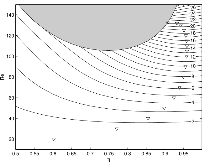
Figure 1: Contours of optimal growth for Taylor-Couette flow in the $(\eta,Re)$ plane. Shaded area indicates the region of linear instability. Triangles indicate $\eta_{\rm opt}(Re)$, the value of $\eta$ at which maximum growth is attained for a given value of Re.

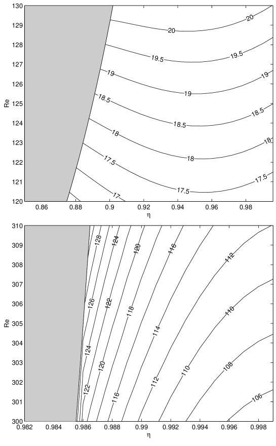
Figure 2: Close-up views of contours of optimal growth. Above: for $120\leq Re\leq 130$, each contour changes slope at a value $\eta_{\rm opt}(Re)\approx 0.96$. Below: for $Re>130$, $G_{\rm max}$ increases as $\eta$ decreases to the linear stability boundary $\eta_{L}$.

We begin by presenting the optimal growth as a function of $\eta$ and $Re$. We recall that throughout our study, we fix the azimuthal wavenumber $m=\alpha=0$, the axial wavenumber $\beta=\pi/2$, and the angular velocity ratio $\mu=-1$. Figure 1 shows the contours of constant optimal growth $G_{\rm max}$. Inside the shaded region, Couette flow is linearly unstable to axisymmetric perturbations. The boundary of this region is the critical Reynolds number $Re_{L}(\eta)$. $Re_{L}\rightarrow\infty$ as $\eta\rightarrow 1$, as expected since plane Couette flow is linearly stable for all Reynolds numbers. We may also consider the rightmost portion of the linear stability boundary as a function $\eta_{L}(Re)$.

A striking feature is that the maximum growth for a fixed Reynolds number, indicated by the triangles in figure 1, is always achieved for a radius ratio $\eta=\eta_{\rm opt}(Re)$ which is less than one. We propose a possible explanation for this trend. As we decrease the radius ratio $\eta$, the asymptotic growth rate, i.e. the imaginary part of the least stable eigenvalue, increases. At the same time, the non-normality of the operator decreases, resulting in diminished transient growth. The combination of these effects results in a maximum growth rate that is achieved for values of $\eta$ less than one. We see that $\eta_{\rm opt}\approx 0.6$ for $Re=20$, increases to a maximum of $\eta_{\rm opt}\approx 0.96$ for $Re\approx 110$, and then abruptly decreases and terminates by meeting the linear instability boundary $\eta_{L}\approx 0.9$ at $Re\approx 130$. For $Re>130$, the maximum growth is achieved for $\eta=\eta_{L}(Re)$. The enlargements in figure 2 show the typical behavior of the contours of $G_{\rm max}$ for $Re$ near 130 and for $Re$ near 300. For $Re\leq 130$, the optimal growth is fairly weak, varying from a factor of 1 to 21. Arbitrarily high values of $G_{\rm max}$ can be attained by increasing $Re$, since for plane Couette flow, i.e. $\eta=1$, it is known Reddygrowth that $G_{\rm max}\sim Re^{2}$. In fact, over the range $300<Re<310$, $G_{\rm max}$ is approximately 20% higher for $\eta=\eta_{L}$ than for $\eta=1$. In this range, the $G_{\rm max}$ contours are nearly vertical as they approach the linear instability boundary, meaning that $G_{\rm max}$ is far more sensitive to a decrease in $\eta$ than to an increase in $Re$. It is near $Re=310$ that plane Couette flow undergoes a sudden unexplained transition to turbulence. Table 2 gives selected numerical values of $G_{\rm max}$.

$\eta$	0.5	0.6	0.7	0.8	0.9	0.95	0.99	0.999	0.9999	Plane
$Re$										Couette
50	1.95	2.39	2.85	3.23	3.38	3.34	3.26	3.23	3.23	3.23
75	2.62	3.51	4.66	5.95	6.90	7.02	6.90	6.85	6.84	6.84
100	3.29	4.69	6.74	9.40	11.70	12.14	12.01	11.93	11.92	11.92
125	4.17	---	---	---	18.45	18.87	18.59	18.46	18.44	18.44
150	5.53	---	---	---	---	27.72	26.65	26.44	26.42	26.42
300	---	---	---	---	---	---	111.60	104.87	104.74	104.73
500	---	---	---	---	---	---	---	291.92	290.39	290.35

Table 2: Optimal growth $G_{\rm max}$ in the narrow-gap limit. Dashed entries indicate linear instability, i.e. $G_{\rm max}=\infty$. Note that, for fixed $Re$, the maximum optimal growth is achieved for $\eta<1$.

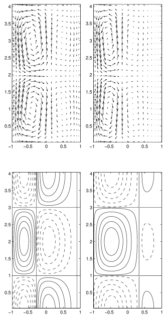
Figure 3: Optimal perturbations for $\eta=0.50$, $Re=125$. Left: optimal input. Right: optimal output. Above: Meridional velocity field $(u_{r},u_{z})$. Below: contours of $u_{\theta}$. The energy of the input (output) is primarily in the meridional (azimuthal) components. For this reason, arrow lengths and contour levels are scaled differently for the input and the output.

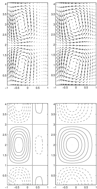
Figure 4: Optimal perturbations for $\eta=0.99$, $Re=350$. Left: optimal input. Right: optimal output. Above: Meridional velocity field $(u_{r},u_{z})$. Below: contours of $u_{\theta}$. The energy of the input (output) is primarily in the meridional (azimuthal) components; arrow lengths and contour levels are scaled differently for the input and the output.

Figure 5: Time evolution of optimal growth. Solid curves denote azimuthal energy $E_{\theta}(t)$, long-dashed curves meridional energy $E_{r,z}(t)$ during evolution from optimal input $\underline{u}(0)$. Higher and lower short-dashed curves represent $E_{\theta}(t)$ and $E_{r,z}(t)$, respectively, for least stable eigenvector. Triangle corresponds to $t_{\rm max}$. Above: $\eta=0.50$, $Re=125$. Below: $\eta=0.99$, $Re=350$.

Figure 6: Square of angular momentum of basic Couette solution $(rU_{\mbox{\tiny}C})^{2}$. Solid curve: $\eta=0.5$, axis on left. Dashed curve: $\eta=0.99$, axis on right. Rayleigh’s criterion for inviscid instability states that $U_{\mbox{\tiny}C}$ is unstable where $(rU_{\mbox{\tiny}C})^{2}$ is a decreasing function of $r$.

We now study in detail two contrasting cases: $\eta=0.5$, $Re=125$ and $\eta=0.99$, $Re=350$. In the first case, $\eta=0.5$ or equivalently $\bar{r}=3$, curvature obviously plays an important role. The second case, $\eta=0.99$ or equivalently $\bar{r}=199$, is very near the plane Couette limit. The Reynolds numbers have been chosen to be close to the linear instability threshold $Re_{L}$ in each case in order to maximize transient growth while remaining within the linearly stable region.

Figures 3 and 4 show the optimal input $\underline{u}(0)$ and output $\underline{u}(t_{\rm max})$ for each case. The least stable eigenvector, i.e. that with the smallest decay rate, is not shown, but resembles the optimal output. The upper portion of each figure shows the meridional velocity fields $(u_{r},u_{z})$ of the optimal input and output, while the lower portion shows contours of azimuthal velocity $u_{\theta}$. The meridional velocity fields consist of vortices whose axes are oriented in the azimuthal direction, similar to the eigenvectors which lead to Taylor vortices at slightly higher Reynolds numbers and to the streamwise vortices which are the optimal inputs in plane Couette flow. The azimuthal components of the optimal inputs and outputs, shown in the lower portions of figures 3 and 4, are in phase opposition with the vortices, with nodal lines at $z=1,3$ going through the vortex centers.

Figure 5 shows the evolution in time of the energies in the meridional components $E_{r,z}$ and in the azimuthal component $E_{\theta}$ starting from the optimal input $\underline{u}(0)$. While the optimal inputs $\underline{u}(0)$ are concentrated primarily in the meridional components, it is the azimuthal component which dominates the optimal outputs $\underline{u}(t_{\rm max})$. For this reason, in order to show the qualitative geometric features of the two fields, the inputs and outputs of Figures 3 and 4 use different scales for the arrow lengths and for the contour levels. This evolution corresponds to the generation of streaks – deformations of the azimuthal velocity profile – by the vortices. This physical process, referred to as the lift-up mechanism, has been described, e.g., in liftup and is believed to be a key element in the transition to turbulence in plane Couette flow.

The graph on the left of figure 5 shows the evolution of $E_{\theta}$ and $E_{r,z}$ starting from the optimal input $\underline{u}(0)$ and from the least stable eigenvector for $\eta=0.50$, $Re=125$. The initial energies are $E_{\theta}(0)=0.2$ and $E_{r,z}(0)=0.8$. Initially, over $0\leq t\leq t_{\rm max}\approx 5$, $E_{\theta}$ rises while $E_{r,z}$ decreases, attaining values of $E_{\theta}(t_{\rm max})\approx 4$ and $E_{r,z}(t_{\rm max})\approx 0.1$, with a ratio $E_{\theta}/E_{r,z}(t_{\rm max})\approx 40$. Over the interval $5\leq t\leq 8$, $E_{r,z}$ increases, while $E_{\theta}$ continues to decrease. With further evolution, both energies decrease as $\underline{u}(t)$ converges towards the least stable eigenvector. From their values at $t=20$, we estimate $E_{\theta}/E_{r,z}(\infty)\approx 0.73/0.023\approx 32$.

The energy evolution for the case $\eta=0.99$, $Re=350$, shown on the right of figure 5, resembles that for plane Couette flow. The optimal input is almost exclusively meridional, with negligible azimuthal component: $E_{r,z}\approx 0.996$ while $E_{\theta}(0)\approx 0.004.$ By $t_{\rm max}\approx 66$, $E_{\theta}$ has increased to 164 and $E_{r,z}$ decreased to 0.14, a ratio $E_{\theta}/E_{r,z}(t_{\rm max})$ of 1170 for the optimal output. This ratio is approximately maintained as both energies slowly decrease during the evolution of $\underline{u}(t)$ towards the least stable eigenvector.

In the case $\eta=0.5$, $Re=125$, two arrays of vortices are present in the optimal input, a larger and stronger array near the inner cylinder and a smaller and weaker array near the outer cylinder. Three arrays are present in the optimal output, whose radial extent and strength decreases in going from the inner to the outer cylinder. In the case $\eta=0.99$, $Re=350$, the optimal input contains one array of vortices and the optimal output contains a second weaker, narrower array near the outer cylinder. Some light can be shed on the form of these perturbation fields and on the difference between the two cases by Rayleigh’s criterion for instability in Taylor-Couette flow.

Rayleigh’s argument, valid for inviscid and axisymmetric flow, is that perturbations interchanging rings of fluid at different radii (e.g. Taylor vortices) will be favored or opposed by the ambient pressure gradient, according to whether the square of the angular momentum $(rU_{\mbox{\tiny}C})^{2}$ decreases or increases radially outwards. For counter-rotating cylinders ($\mu<0$), the sign of $d(rU_{\mbox{\tiny}C})^{2}/dr$ changes within the gap. Rayleigh’s criterion is then applied to argue that only the inner portion of the gap is unstable. This modification is justified by three related tendencies DrazinReid . First, the unstable eigenvector is concentrated near the inner cylinder, where $d(rU_{\mbox{\tiny}C})^{2}/dr$ is negative. Second, the axial wavelength corresponding to the most unstable or least stable eigenvector decreases, favoring vortices which remain closer to circular. Third, the critical Reynolds number for linear instability increases, meaning that the critical Reynolds number based on the unstable portion of the gap remains nearly constant.

Figure 6 shows that the square of the angular momentum decreases radially outwards over the interval $r\lesssim\bar{r}-0.5$ for $\eta=0.50$ and over the interval $r\lesssim\bar{r}$ for $\eta=0.99.$ Although exact application of Rayleigh’s criterion would lead to optimal perturbations far more concentrated near the inner cylinder than they actually are, the criterion provides a heuristic explanation for the asymmetry. Rayleigh’s criterion is usually invoked to explain linear instability, i.e. exponential growth. However, a modified version of the criterion should apply to transient growth as well.

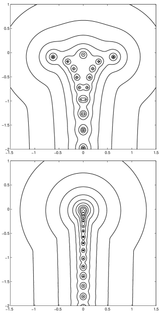
Figure 7: Pseudospectra for Taylor-Couette flow. Above: $\eta=0.5$ and $Re=125$. Contours correspond to $\epsilon=10^{-1.8},10^{-1.5},\ldots,10^{0}$. Below: $\eta=0.99$ and $Re=350$. Contours correspond to $\epsilon=10^{-2.4},10^{-2.1},\ldots,10^{0}$.

Finally, we show the spectrum and pseudospectra of the operators ${\cal L}$ for the two cases in figure 7. Both pseudospectra plots contain contours (for the smaller values of $\epsilon$) surrounding individual eigenvalues and bulb-shaped contours (for the larger values of $\epsilon$) surrounding the entire spectrum. For both values of $\eta$, the contours for a fixed small value of $\epsilon$ surrounding the eigenvalues near the real axis are wider than the contours surrounding the eigenvalues farther from the real axis. The bulb-shaped contours, however, differentiate between the two values of $\eta$. The spectrum for $\eta=0.5$ contains eigenvalues near the real axis with real parts extending to approximately $\pm 0.7;$ a bulb-shaped pseudospectral contour thus remains a fairly constant distance from the spectrum. The spectrum for $\eta=0.99$ is, in contrast, quite localized on the imaginary axis; in this case, a bulb-shaped pseudospectral contour protruding into the unstable half-plane is a first indication of non-normal effects.

We use more detailed calculations of the pseudospectra to compute approximations to the lower bound (14) on optimal growth of Kreiss’ theorem. For $\eta=0.5$, we obtain an upper bound ${\rm Im}(z)\leq 0.1$ for the $\epsilon$-pseudospectrum with $\epsilon=10^{-1.15}$, which yields the lower bound $G_{\rm max}\geq(10^{1.15}\times 0.1)^{2}=1.99$, about half of the exact value $G_{\rm max}=4.17$ that we have calculated. For $\eta=0.99$, we obtain an upper bound ${\rm Im}(z)\leq 0.03$ for the $\epsilon$-pseudospectrum with $\epsilon=10^{-2.45}$, which yields the lower bound $G_{\rm max}\geq(10^{2.45}\times 0.03)^{2}=71.49$, again about half of the exact value of 155.

IV Conclusions

We have calculated the pseudospectra and optimal transient growth for Taylor-Couette flow.

Our major result is that, for a fixed Reynolds number, the optimal transient growth is achieved for a radius ratio $\eta=\eta_{\rm opt}<1$, rather than for the plane Couette limit $\eta=1$. This is due to the combined effect of increasing modal growth and decreasing non-normality. As shown in figure 1, for $Re<130$, the optimal transient growth for fixed $Re$ occurs at an intermediate value of $\eta$ ranging from $\eta_{\rm opt}=0.6$ at $Re=20$ to $\eta_{\rm opt}=0.96$ at $Re=110$. For $Re>130$, the optimal transient growth for fixed $Re$ increases as $\eta$ is decreased from the plane Couette limit $\eta=1$ to the linear stability boundary $\eta=\eta_{L}$, as shown in figure 2.

If transient growth on the order of $G_{\rm max}\approx 100$ is suspected to initiate transition in plane Couette flow near $Re=300$, then transition should also occur near $Re=300$ outside the linear instability domain in Taylor-Couette flow, albeit in very narrow gaps ($\eta\gtrsim 0.986$). If these predictions fail to hold, then theories concerning transition initiated by transient growth must be modified or even abandoned. Another possible direction for future studies concerns regions of $(\eta,Re)$ in which transient growth competes with linear instability; such situations should be included in a comprehensive theory of transition initiated by non-normal effects.

Two cases have been considered in detail: $\eta=0.99$, $Re=350$ and $\eta=0.5$, $Re=125$. Both show transient growth. As could be expected, the case $\eta=0.99$, $Re=350$, shows much higher transient growth, both because of its greater resemblance to plane Couette flow and also because of its higher Reynolds number. As shown in figure 5, for $\eta=0.99$, $Re=350$, energy grows from the optimal input by a factor of $G_{\rm max}=164$, while for $\eta=0.5$, $Re=125$, we have $G_{\rm max}=4$.

As is the case for plane Couette flow, the physical mechanism accompanying transient growth consists of the conversion of vortices (here, termed azimuthal rather than streamwise) into streaks, i.e. perturbations of the basic Couette profile. This is seen in the ratio of azimuthal to meridional energy in figure 5 of the optimal inputs $\underline{u}(0)$ and outputs $\underline{u}(t_{\rm max})$. The optimal outputs, depicted in figures 3 and 4, are of higher amplitude near the inner cylinder, especially in the case $\eta=0.5$, $Re=125$, as indicated by Rayleigh’s criterion for centrifugal instability illustrated in figure 6.

Although both sets of pseudospectra in figure 7 show signs of non-normality, those for $\eta=0.99$, $Re=350$ show more deviation from the spectrum than those for $\eta=0.5$, $Re=125$.

Our study is restricted to the azimuthal wavenumber $m=\alpha=0$, axial wavenumber $\beta=\pi/2$ and angular velocity ratio $\mu=-1$. Previous results on Couette flows lead us to believe that these values of $(\alpha,\beta)$ may be representative of a fairly large portion of parameter space, since both the maximal optimal growth rate in plane Couette flow and the maximal linear growth rate in Taylor Couette flow are close to those achieved for $\alpha=0$, $\beta=\pi/2$. Varying $\mu$, however, leads to major qualitative changes, as it does in other aspects of Taylor-Couette flow. Studies encompassing a wide range of parameter values Meseguer are clearly desirable.

In the words of Faisst & Eckhardt Eckhardt , Taylor-Couette flow provides an ”embedding” of plane Couette flow. Numerical simulations and laboratory experiments have extensively documented the way in which plane Couette flow changes as its single non-dimensional parameter, the Reynolds number, is increased. Taylor-Couette flow provides an ensemble of other parameter paths along which to approach or to step back from plane Couette flow. Our hope is that this preliminary study and that of Meseguer of transient growth and pseudospectra in Taylor-Couette flow, will help to increase understanding of both Taylor-Couette flow and of the effects of non-normality.

Acknowledgments

We gratefully acknowledge Thomas Wright for use of his code for calculating pseudospectra, and Satish Reddy for use of his code for calculating optimal growth. PJS thanks Patrick Huerre and the people at LadHyX for their warm hospitality during his sabbatical stay.

References

- (1) G.I. Taylor, Stability of a viscous fluid contained between two rotating cylinders, Phil. Trans. Roy. Soc. London, Ser. A, 223, 289–343, (1923).
- (2) D. Coles, Transition in circular Couette flow, J. Fluid Mech. 21, 385–425 (1965).
- (3) C.D. Andereck, S.S. Liu & H.L. Swinney, Flow regimes in a circular Couette system with independently rotating cylinders, J. Fluid Mech. 164, 155–183 (1986).
- (4) R. Tagg, W.S. Edwards, H.L. Swinney & P.S. Marcus, Nonlinear standing waves in Couette-Taylor flow, Phys. Rev. A 39, 3734–3737 (1989).
- (5) E.R. Krueger, A. Gross & R.C. DiPrima, On the relative importance of Taylor-vortex and non-axisymmetric modes in flow between rotating cylinders, J. Fluid Mech. 24, 521–538, (1966).
- (6) P.S. Marcus, Simulation of Taylor-Couette flow. II. Numerical results for wavy-vortex flow with one traveling wave, J. Fluid Mech. 146, 65–113 (1984).
- (7) W.F. Langford, R. Tagg, E.J. Kostelich, H.L. Swinney & M. Golubitsky, Primary instabilities and bicriticality in flow between counter-rotating cylinders, Phys. Fluids 31, 776–785 (1988).
- (8) R.C. DiPrima & H.L. Swinney, Instabilities and transition in flow between concentric rotating cylinders, in Hydrodynamic Instabilities and the Transition to Turbulence, ed. by H.L. Swinney and J.P. Gollub, Springer-Verlag, New York (1981).
- (9) P.G. Drazin & W.H. Reid, Hydrodynamic Stability, Cambridge University Press, Cambridge, U.K. (1981).
- (10) R. Tagg, The Couette-Taylor Problem, Nonlinear Science Today 4, 1–25 (1994).
- (11) P. Chossat & G. Iooss, The Couette-Taylor Problem, Springer-Verlag, New York (1994).
- (12) H.B. Squire, On the stability for three-dimensional disturbances of viscous fluid flow between parallel walls, Proc. Roy. Soc. Lond. Ser. A 142, 621–628 (1933).
- (13) V.A. Romanov, Stability of plane-parallel Couette flow, Funkcional Anal. i Prolozen 7, 62–73, translated in: Functional Anal. & Its Appl., 7, 137–146 (1973).
- (14) N. Tillmark & P.H. Alfredsson, Experiments on transition in plane Couette flow, J. Fluid Mech. 235, 89–102 (1991).
- (15) A. Lundbladh & A. V. Johansson, Direct simulation of turbulent spots in plane Couette flow, J. Fluid Mech. 229, 499–516 (1991).
- (16) D.D. Joseph, Nonlinear stability of the Boussinesq equations by the method of energy, Arch. Rat. Mech. Anal. 22, 163–184 (1966).
- (17) K.M. Butler & B.F. Farrell, Three-dimensional optimal perturbations in viscous shear flow, Phys. Fluids A 4, 1637–1649 (1992).
- (18) L.N. Trefethen, A.E. Trefethen, S.C. Reddy, and T.A. Driscoll, Hydrodynamic stability without eigenvalues, Science 261, 578–584 (1993).
- (19) S.C. Reddy & D.S. Henningson, Energy growth in viscous channel flows, J. Fluid Mech. 252, 209–238 (1993).
- (20) F. Waleffe, Transition in shear flows. Nonlinear normality versus nonnormal linearity, Phys. Fluids 7, 3060–3066 (1995).
- (21) T. Gebhardt & S. Grossmann, The Taylor-Couette eigenvalue problem with independently rotating cylinders, Zeitschrift für Physik B 90, 475–490 (1993).
- (22) A. Meseguer, Energy transient growth in the Taylor-Couette problem, Phys. Fluids 14, 1655–1665.
- (23) M. Nagata, Three-dimensional finite-amplitude solutions in plane Couette flow: bifurcation from infinity, J. Fluid Mech., 217 519–527 (1990).
- (24) M. Nagata, Tertiary solutions and their stability in rotating plane Couette flow, J. Fluid Mech. 358, 357–378 (1998).
- (25) H. Faisst & B. Eckhardt, Transition from the Couette-Taylor system to the plane Couette system, Phys. Rev. E 61, 7227–7230 (2000).
- (26) A. Prigent, G. Grégoire, H. Chaté, O. Dauchot & W. van Saarloos, Large-scale finite-wavelength modulation within turbulent shear flows, Phys. Rev. Lett. 89, 014501 (2002).
- (27) C. Canuto, M. Y. Hussaini, A. Quarteroni & T. A. Zang, Spectral Methods in Fluid Dynamics, Springer-Verlag, Berlin (1988).
- (28) S.C. Reddy, P.J. Schmid & D.S. Henningson, Pseudospectra of the Orr-Sommerfeld operator, SIAM J. Appl. Math. 53, 15–47 (1993).
- (29) P.J. Schmid & D.S. Henningson, Stability and Transition in Shear Flows, Springer-Verlag, New York, 2001.
- (30) L.N. Trefethen, Computation of Pseudospectra, Acta Numerica 8, 247–295 (1999).
- (31) T.G. Wright & L.N. Trefethen, Large-scale computation of pseudospectra using ARPACK and Eigs, SIAM J. Sci. Comp. 23, 591–605 (2001).
- (32) M.T. Landahl, A note on an algebraic instability of inviscid parallel shear flows, J. Fluid Mech. 98, 243–251 (1980).