Quantum chaos in optical systems: The annular billiard

Abstract

We study the dielectric annular billiard as a quantum chaotic model of a micro-optical resonator. It differs from conventional billiards with hard-wall boundary conditions in that it is partially open and composed of two dielectric media with different refractive indices. The interplay of reflection and transmission at the different interfaces gives rise to rich dynamics of classical light rays and to a variety of wave phenomena. We study the ray propagation in terms of Poincaré surfaces of section and complement it with full numerical solutions of the corresponding wave equations. We introduce and develop an $S$-matrix approach to open optical cavities which proves very suitable for the identification of resonances of intermediate width that will be most important in future applications like optical communication devices. We show that the Husimi representation is a useful tool in characterizing resonances and establish the ray-wave correspondence in real and phase space. While the simple ray picture provides a good qualitative description of certain system classes, only the wave description reveals the quantitative details.

]

I Introduction

Billiard systems of many kinds have proven to be very fruitful model systems in the field of quantum chaos. The methods of investigation are well established both for the classical dynamics and for the quantum mechanical behaviour, with semiclassical methods describing the transition from quantum to classical properties. With the growing interest in quantum chaos and in mesoscopic physics, new systems have entered the stage, including systems exhibiting chaos of classical waves such as (macroscopic) microwave billiards [2, 3], acoustic resonators [4] as well as deformed microcavities [6, 7, 8, 9, 10, 11] which can operate as microlasers [12, 13]. To describe these (two-dimensional) systems one can exploit the analogy between the stationary Schrödinger equation and the Helmholtz equation for (classical) waves [14]. Quantum chaotic experiments using microwave cavities or other classical waves (e.g., acoustic or water waves) are based on this mathematical equivalence, see [15] for a review. Most of the investigated systems are hard-wall billiards. However, for the class of optical, or dielectric, model systems the billiard boundary manifests itself by a change in the index of refraction allowing for reflection and transmission of light. The limit of closed systems is approached as the difference in the refractive indices reaches infinity.

We emphasize that the openness of optical systems extents the set of interesting questions with respect to those for closed billiards. In this paper we suggest a further extension of the class of open optical cavities by considering two regions with different refractive indices inside the cavity, which leads to an additional refractive interface between the two dielectrics inside the resonator. The interplay between refraction inside the billiard and partial reflection at the outer billiard boundary gives rise to a variety of phenomena in the classical ray dynamics and correspondingly in the wave description of such systems.

The model we study is the annular billiard shown in Fig. 1. It consists of a small disk of radius $R_{2}$ placed inside a larger disk of radius $R_{1}$ with a displacement $\delta$ of the disk centres. This system is well-known from quantum and wave mechanical studies of the hard-wall configuration [16, 17, 18] with non-vanishing wave-functions only in the annular region. It carries features of a ray-splitting system [19] when each disk is characterized by a (stepwise constant) potential (unlike the situation we will discuss here, see Sec. II B). Here we consider disks characterized by indices of refraction, $n_{1}$ and $n_{2}$, respectively, with the index of the environment fixed at $n_{0}=1$ [20]. We will study billiard materials with $n_{i}>1$ such that confinement by total internal reflection is possible. Then methods well-known from the description of classical dynamical systems, such as the use of Poincaré’s surfaces of section, can be employed to describe the ray dynamics. Note that whispering gallery modes in the dielectric annular billiard with a metallic inner disk have been discussed in Ref. [21]. A detailed study of periodic orbits in a specific hard-wall configuration, together with the expected consequences on the electromagnetic scattering problem was performed in Ref. [22].

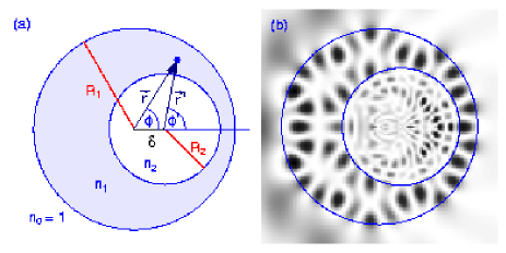
FIG. 1.: (a) Geometry and notations of the dielectric annular billiard. (b) Example of a resonant wave function excited by a plane wave with wave number $k=6.251$ incident from the left ($R_{1}=1,R_{2}=0.6,\delta=0.22,n_{1}=3,n_{2}=6$). Dark regions denote high electric field intensity.

The above-mentioned correspondence between the Helmholtz and Schrödinger equation is established by means of an effective potential [23] that depends not only on position and the respective index of refraction $n$, but also on the energy. Changes in the refractive index give rise to steps in the effective potential which allows for a quantum-mechanical interpretation (e.g., quasibound states, tunneling escape). We will discuss this point in the next section when we contrast optical systems governed by Maxwell’s equation with quantum mechanical problems obeying the Schrödinger equation. Also, we will see how the two possible polarization directions affect the Maxwell-Schrödinger correspondence and which quantity takes the role of $\hbar$: Maxwell’s equations are, of course, not aware of the existence of $\hbar$.

The further outline of the paper is as follows: In Sec. II we introduce the ray and wave optics notion for the simple system of the dielectric disk that arises from the annular system upon removal of the inner obstacle ($n_{1}=n_{2}$, or $R_{2}=0$). We describe the methods used for the study of the annular billiard in the subsequent sections; namely the adaptation of the Poincaré surface of section method, well-known from classical mechanics, to optical systems, the exact solution of the Maxwell equation (leading to an effective Schrödinger equation), and the $S$-matrix approach. Whereas the first approach is based on the ray picture, the latter two clearly fully include the wave nature of light. We employ these methods for the annular billiard in Sec. III, where we introduce methods to study the ray dynamics in optical compound systems and apply, for the first time to our knowledge, an $S$-matrix formalism to optical billiards. The expected ray-wave, or classical-quantum, correspondence is established in Sec. IV and investigated from various viewpoints, including both real space and phase space arguments. However, several features in the behaviour of waves require improvements of the simple ray model as we will illustrate and explain with typical examples. In our conclusion, Sec. V, we discuss the possibility of an experimental realization of the annular system with the currently available dielectric materials. The successes of the ray-picture illuminated here and elsewhere [6, 7, 11, 13, 24] suggest the ray-based design of micro-optical cavities for, e.g., future communication technologies.

II The dielectric disk

In this section we introduce the methods, techniques, and notations used later in the discussion of the annular billiard. We present the ray and wave picture for the description of optical (or dielectric) systems using the simple example of a dielectric disk, which provides all the ingredients to deal with the annular billiard (apart from a coordinate transformation, see below). We start with the ray optics approach and show how methods well established in classical dynamics can be adopted to optical systems. In the wave description we distinguish between an approach to the resonant states of the (naturally) open optical system by complex wave vectors based on Maxwell’s equations on the one hand, and by real wave vectors arising in an $S$-matrix approach on the other hand.

A Ray Optics: Classical billiards with total internal reflection

Within ray optics, the zero-wavelength limit of wave optics, light is described by a ray that follows a straight line through a medium, very similar to the dynamics of a point mass. Let us assume a light ray, or plane wave, incident under an angle $\chi_{1}$ with respect to the normal of a dielectric boundary where the refractive index changes from $n_{1}$ to $n_{2}$. At the interface, the ray is i) specularly reflected under an angle $\chi_{2}=\chi_{1}\equiv\chi$, with a polarization-dependent [25] probability $R^{\rm TM/TE}$, see Fig. 2(b). The remaining part, $T^{\rm TM/TE}=1-R^{\rm TM/TE}$, is ii) transmitted into the other medium under an output angle $\eta$ given by Snell’s law, $\sin\eta=(n_{1}/n_{2})\sin\chi\equiv n\sin\chi$. In the last identity we have employed the scaling properties of the system that allow one to fix one of the refractive indices, (e.g. that of the environment) to unity without loss of generality.

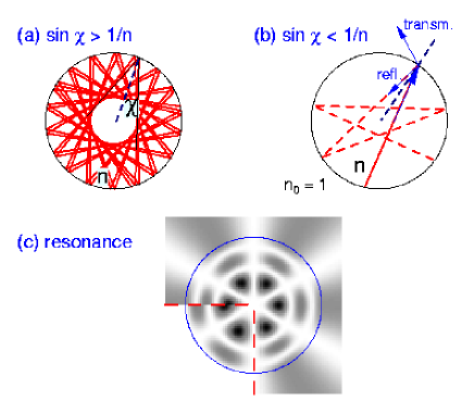
FIG. 2.: Comparison of ray and wave picture for a dielectric disk of refractive index $n$. The upper panels illustrate the two possibilities of (a) total internal reflection, $\sin\chi\geq\sin\chi_{c}=1/n$, when the ray dynamics is equal to that of a classical point particle in a closed system, and (b) ray refraction when, due to partial transmission, the light intensity inside the disk decreases with time. In (c) the intensity of the electric field (see Sec. II B, higher intensity in darker regions) for a quasibound state ($nkR=11.428-0.254{\rm i}$) of the dielectric disk ($n=3$) is shown. For comparison, an eigenstate of the closed disk ($nkR=9.761$, vanishing intensity outside the disk) is given in the lower left sector (both are for transverse magnetic field, TM polarization).

Snell’s law cannot be fulfilled to yield real $\eta$ for any angle of incidence $\chi$ if $n>1$ ($n_{1}>n_{2}$, respectively). Total internal reflection occurs if $\sin\chi\geq\sin\chi_{c}\equiv 1/n$ where we introduced the critical angle $\chi_{c}$. For angles of incidence above the critical angle, light is confined by total internal reflection with zero transmission and behaves like a classical point particle, Fig. 2(a). Therefore, real and phase space methods from classical mechanics (such as ray tracing or the Poincaré surface of section technique), prove to be very useful if they are complemented by the optical property of refraction: The Poincaré surface of section (SOS) method works exact (except for the exponentially small tunneling losses) as long as we are in the regime of total internal reflection. However, for $-1/n<\sin\chi<1/n$, light can escape so that the intensity remaining inside the disk is diminishing. This fact has to be taken into account when discussing the Poincaré SOS for optical systems. Figure 3 shows an example of a Poincaré SOS for a hard-wall annular system with slightly eccentric inner disk ($\delta=0.01$). The critical value $\sin\chi=1/n$ is marked by an arrow.

Probing the phase space structure of a rotational invariant system like a disk in terms of a Poincaré SOS gives a uniform structure as shown in the upper part of Fig. 3. Although this is a Poincaré SOS for an annular system [26] with a slightly eccentric inner disk (see Sec. IV), it is identical to that for a disk for trajectories that do not hit the inner disk, i.e. $\sin\chi>R_{2}+\delta$ ($R_{1}=1$). The straight horizontal lines directly express the conservation of angular momentum, that is, conservation of $\sin\chi$, and the corresponding trajectories are referred to as whispering gallery (WG) orbits.

The reflection and transmission probabilities, $R^{\rm TM/TE}$ and $T^{\rm TM/TE}$, are provided by Fresnel’s laws [27]. A plane electromagnetic wave incident on a planar dielectric interface with angle of incidence $\chi$ is reflected with the polarization-dependent probabilities

$$R^{\rm TM}=\frac{\sin^{2}(\chi-\eta)}{\sin^{2}(\chi+\eta)}\>,\quad R^{\rm TE}=\frac{\tan^{2}(\chi-\eta)}{\tan^{2}(\chi+\eta)}\>,$$ (1)

where TM (TE) denotes transverse polarization of the magnetic (electric) field at the interface, and $\eta=\arcsin(n\sin\chi)$ is the direction of the refracted beam according to Snell’s law.

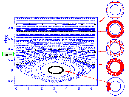
FIG. 3.: Poincaré surface of section for the annular billiard with $R_{1}=1,R_{2}=0.6$, and $\delta=0.01$. The horizontal axis is the polar angle $\phi$, the vertical axis, $\sin\chi$, is proportional to the angular momentum in $z$-direction (perpendicular to the system plane). Although the displacement of the inner disk is rather small, it has major impact on trajectories that explore the region $\sin\chi<R_{2}+\delta$. Other trajectories are not influenced and identical to those of a single dielectric disk, see e.g. the two upper-most examples on the right. The initial angular momentum of the trajectories shown is positiv ($\sin\chi>0$). Nonetheless regions where $\sin\chi<0$ are explored, implying a change in the sense of rotation as, e.g., in the lower-most trajectory on the right. The critical angle for total internal reflection is marked on the left indicating that the two lower-most trajectories are not confined.

B Wave Picture: From Maxwell to Schrödinger

Before we turn to the more complicated annular billiard in Sec. III, we assume an infinite dielectric cylinder of radius $R$ and refractive index $n$ embedded in vacuum with refractive index $n_{0}=1$. We will call $k$ the wave number outside the cylinder and, analogously, $nk$ is the wave number inside. The solution of Maxwell’s equations for the vortices of the electromagnetic field [27] is given, e.g., in Refs. [5, 23], and leads to an equation for the electric (magnetic) field that is similar to the conventional Schrödinger equation. The vector character of the fields implies, however, that one has to distinguish two possible polarization directions with differing boundary conditions. The situation where the electric (magnetic) field is parallel to the cylinder ($z$-) axis is called TM (TE) polarization, with the magnetic (electric) field being thus transverse. Using the rotational invariance of the system, separation in cylindrical variables (assuming a $\phi$-dependence $e^{im\phi}$, and a $z$-dependence $e^{ik_{z}z}$) eventually leads to an effective Schrödinger equation [28] for the radial component of the electric field,

$$-\left[\frac{d^{2}}{dr^{2}}+\frac{1}{r}\frac{d}{dr}\right]E(r)+V_{\rm eff}(r)E(r)=k^{2}E(r),$$ (2)

where we introduced the effective potential

$$V_{\rm eff}(r)=k^{2}(1-n^{2})+m^{2}/r^{2}+k_{z}^{2}\>.$$ (3)

The first term reveals immediately that dielectric regions with $n>1$ correspond to an attractive well in the quantum analogy, and that a potential structure is determined by the change of the refractive indices for different regions. Note, however, the energy-dependent prefactor – a far-reaching difference in comparison to quantum mechanics. The other two terms in Eq. (3) arise from the conservation of the angular momentum (characterized by the quantum number $m$), and express the conservation of the linear momentum along the cylinder axis (acting as an offset in energy), respectively.

In the following we will consider a dielectric disk (that is, we choose a particular cross sectional plane of the cylinder to obtain an effective system), and set $k_{z}$ to zero corresponding to a wave in the $x$-$y$ plane. Approaching the disk from the outside ($r>R,n_{0}=1$) there is only the angular momentum contribution to the effective potential $V_{\rm eff}$, Eq. (3). At $r=R$, there is a discontinuity in $V_{\rm eff}$ that is proportional to $1-n^{2}$, reflecting the non-continuous change in the refractive index. It reaches from $k_{\rm max}^{2}=m^{2}/R^{2}$ to $k_{\rm min}^{2}=m^{2}/(n\,R)^{2}$. Inside the disk the angular momentum contribution, now shifted by $k_{\rm max}^{2}-k_{\rm min}^{2}$, again determines the behaviour (see also Fig. 9 at values $r/R_{1}>R_{2}/R_{1}$ ).

The form of the potential suggests an interpretation in the spirit of quantum mechanics with metastable states in the potential well that decay by tunneling escape, and indeed this turns out to be the quantum-mechanical version of confinement by total internal reflection [5, 23]. To this end we employ a semiclassical quantization condition for the $z$-component of the quantum mechanical and classical angular momentum, $m\hbar=n\hbar{\rm Re}(kR)\sin\chi$. We find

$$\sin\chi=\frac{m}{n{\rm Re}(kR)}\>$$ (4)

as relation between the angle of incidence as ray picture quantity, and the wave number and angular momentum of a resonance.

Another correspondence between ray and wave quantities exists between the (polarization-dependent) Fresnel reflection coefficient $R^{\rm TM/TE}$ and the imaginary part of the wave number that describes the decay of a resonant state. In fact one can deduce a reflection coefficient $R_{d}^{\rm TM/TE}$ of the disk [29],

$$R^{\rm TM/TE}_{d}=\exp[4n\,{\rm Im}(kR)\cos\chi]\>.$$ (5)

We wish to point out that there exist deviations between the Fresnel values $R^{\rm TM/TE}$ and $R^{\rm TM/TE}_{d}$ when the wavelength becomes comparable to the system size, in particular around the critical angle. This can be understood within a semiclassical picture based on the Goos-Hänchen effect [30, 31].

The general solutions of the radial Schrödinger equation (2)  are Bessel and Neumann functions, $J_{m}(k_{i}r)$ and $Y_{m}(k_{i}r)$ of order $m$, where $k_{i}$ is the wave number in the respective medium. Since physics requires a finite value of the wave function at the disk center, the solution inside the disk can consist of Bessel functions only. Outside the dielectric we assume an outgoing wave function, namely a Hankel function $H_{m}^{(1)}$ of the first kind, in accordance with our picture of a decaying state. The resonant states are obtained by matching the wave field $\propto J_{m}(nkr)e^{im\phi}$ inside the disk at $r=R$ to the wave field $\propto H_{m}^{(1)}(kr)e^{im\phi}$ outside the disk according to the polarization dependent matching conditions deduced from Maxwell’s equations. The resonant states are solutions of

$$J_{m}(nkR)\,{H_{m}^{(1)}}^{\prime}(kR)={\cal P}\,J^{\prime}_{m}(nkR)\,H_{m}^{(1)}(kR)\>,$$ (6)

where ${\cal P}=n$ ($1/n$) for TM (TE) polarization (primes denote derivatives with respect to the full arguments $nkr$ and $kr$, respectively).

One example of a quasibound state as solution of the optically open system is shown in Fig. 2(c) and compared to a solution of the closed disk. The shift in the wave patterns is clearly visible. Owing to the symmetry of the system we find a characteristic (quantum-mechanical) node structure that is directly related to the quantum numbers $m$ (there are 2$m$ azimuthal nodal points), and $\rho$ counting the radial nodes (hence $m=3,\rho=2$ in the example).

At this point a further discussion concerning the appearance of $\hbar$ in optical systems is convenient. Employing the quantum-classical correspondence, one expects $\hbar$ to be related to the reciprocal wave number, $\hbar\sim 1/k$, because $\hbar\to 0$ in the classical (here the ray) limit $k\to\infty$. This relation is indeed obtained when we compare Eq. (2), divided by $k^{2}$ (thereby removing the energy-dependence of the effective potential), with Schrödinger’s equation, and identify $1/k$ with $\hbar$.

C $S$-Matrix approach to the dielectric disk

The main idea when considering a scattering problem is to probe the response of the system to incoming (test) waves, and to extract system properties like resonance positions and widths from the scattered wave. Physically, this method is formulated for real wave vectors.

Here we want to investigate the scattering properties of the dielectric disk for electromagnetic waves in the framework of $S$-matrix theory [32, 33, 34]. One possible choice for the incident test waves are, of course, plane waves. For our rotational invariant disk of finite dimension, however, incident waves that allow for angular momentum classification are much more convenient: Then we need to take into consideration only waves with impact parameter of the order of the system dimension or smaller. The Hankel functions $H_{m}^{(2)}$ of the second kind possess the desired properties.

Again, we consider a dielectric disk of radius $R$ and refractive index $n$ and denote the vacuum wave number by $k$. According to Maxwell’s equations and the discussion in the previous Sec. II B we write the wave function $\Psi_{m}^{\rm scatt}$ outside that is excited by an incident wave of angular momentum $m$ as

$\displaystyle\Psi_{m}^{\rm scatt}(kr)=H_{m}^{(2)}(kr)e^{im\phi}+\sum_{l=-\infty}^{\infty}S_{ml}H_{l}^{(1)}(kr)e^{il\phi}\>.$

Here, $S_{ml}$ is the amplitude for an incident wave $H_{m}^{(2)}$ to be scattered into $H_{l}^{(1)}$. The scattering amplitudes are comprised in the $S$-matrix. It follows from flux conservation that $S$ has to be unitary, a property that we will use subsequently. Starting with a general situation in which $S$ can have entries everywhere, symmetry requirements will reduce the number of independent matrix elements. For the dielectric disk, the scattered wave has to obey angular momentum conservation and will, therefore, be a Hankel function of the same order $m$ as the incoming Hankel function. Hence the scattering matrix is diagonal. In the general case where angular momentum is not conserved (as, for example, for a deformed disk or the annular geometry that we will consider in all following sections), scattering will occur into all possible angular momenta $l$.

Employing the matching conditions (cf. Sec. II B) for TM polarization, we obtain from the requirement of continuity of the wave function (or the electric field) and their derivative eventually the matrix elements $S_{mm^{\prime}}$:

$$S_{mm^{\prime}}=-\frac{{H_{m}^{(2)}}^{\prime}(kr)-n\frac{J^{\prime}_{m}(nkr)}{J_{m}(nkr)}{H_{m}^{(2)}}(kr)}{{H_{m}^{(1)}}^{\prime}(kr)-n\frac{J^{\prime}_{m}(nkr)}{J_{m}(nkr)}{H_{m}^{(1)}}(kr)}\>\delta_{mm^{\prime}}\>.$$ (7)

The general idea for identifying resonances is that a probing wave with resonance energy will interact longer with the system than a wave with “non-fitting” energy. This can be quantified in terms of the Wigner delay time $\tau^{W}(E_{k})$ [35] that is the derivative of the total phase $\theta$ of the determinant of the $S$-matrix, det$S$=$e^{i\theta}$, with respect to energy $E_{k}=k^{2}$,

$$\tau^{W}(E_{k})=\frac{d\theta(E_{k})}{dE_{k}}\>.$$ (8)

In the following, we will use the wave-number based delay time

$$\tau(k)\equiv 4\pi\,k\>\tau^{W}(k^{2})$$ (9)

in order to identify resonances as depicted in Fig. 4(a). The solid line shows the result for a dielectric disk with $n$=3. Families of whispering gallery modes (WGMs) are identified upon increasing the wave number and can be labelled by the quantum number $m$ that counts the azimuthal nodes (2$m$). The decrease in peak width, accompanied by an increase in height, that is observed with increasing $m$ corresponds to an increase of the angle of incidence, Eq. (4), and improved confinement by total internal reflection.

Note the relation between the (total) phase $\theta(E_{k})$ of the $S$-matrix and the so-called resonance counting function: $N(E_{k})=\theta(E_{k})/2\pi$, cf. [32]. The idea is that a resonance is encountered whenever the phase $\theta$ of $\det S$ increases by $2\pi$ upon increasing the energy $E_{k}$.

In the following we will use the function $\tau(k)$ to determine the resonances. Isolated resonances appear as (Lorentzian) peaks in $\tau(k)$, see Fig. 4(a), above a small background. Information about the imaginary part of the resonance is now encoded in the height and width of the Lorentzian resonance peaks [33]. We point out that the resolution of very broad and extremely narrow resonances might be difficult, because they are either included in the background or not captured using a finite numerical grid interval. However, resonances with a wide range of widths are easily identified, in particular all resonances that are of interest for microlaser applications are found within the $S$-matrix approach [36].

The area under the curve $\tau(k)$ is proportional to the number of states with wave numbers smaller than $k$ [32, 34]. In the case of stepwise potentials such as realized in ray-splitting billiards, simple Weyl formulas for the smooth part of the density of states were derived for a number of geometries [19]. The application of these results to optical systems where ray splitting is realized by refraction and transmission at refractive index boundaries is tempting. However, here we work with an energy dependent effective potential, in contrast to the situation studied in [19] where only a (stepwise) spatial dependence of the potential was assumed. Consequently, a generalization of the formulas derived in [19] would be required if one is interested in an analytical expression for the smooth part of the density of states, which is, however, not the subject of this work.

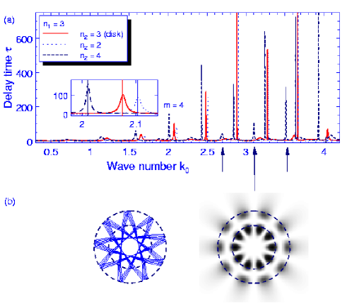
FIG. 4.: (a) Resonances in the concentric annular billiard ($R_{1}=1,R_{2}=0.6,n_{1}=3$), corresponding to the first family of whispering gallery modes. The annular systems $n_{2}=2$ (dotted) and $n_{2}=4$ (dashed) are compared with the homogeneous disk $n_{2}=3$. Note the systematic deviation of the resonance position to larger (smaller) wave numbers for $n_{2}=2$ ($n_{2}=4$) that decreases with increasing angular momentum quantum number $m$ since the inner disk becomes less important. In the inset, we compare the positions and widths of the 4th resonance ($m=4$) in the delay time with the respective complex wave numbers according to Eq. (11). We find excellent agreement with the numerically exact values $k_{0}=2.0108-0.0041{\rm i}$ ($n_{2}=4$), $k_{0}=2.0753-0.0063{\rm i}$ ($n_{2}=3$), and $k_{0}=2.1035-0.0075{\rm i}$ ($n_{2}=2$). Note the existence of additional resonances for $n_{2}=4$, some of them marked by arrows from below and illustrated in the ray and wave picture in (b). They are due to the double-well structure of the effective potential and referred to as “double WGMs”, see text.

III Annular billiard in the ray and wave picture

In this section we adopt the ray and wave methods explained above to the general case of the dielectric annular billiard. We will denote the three different regions, namely the environment (refractive index $n_{0}$), the annular region ($n_{1}$), and the inner disk ($n_{2}$) by the indices 0, 1, and 2, respectively. The corresponding wave numbers are $k_{0},k_{1}$, and $k_{2}$. Due to the scaling properties we fix $n_{0}\equiv 1$ and one of the geometry parameters $R_{1},R_{2},\delta$; we choose $R_{1}\equiv 1$. Given a set of parameters ($n_{0}\equiv 1,n_{1},n_{2}$), the same results hold for the scaled set ($\widetilde{n}_{0},\widetilde{n}_{1}=n_{1}\widetilde{n}_{0},\widetilde{n}_{2}=n_{2}\widetilde{n}_{0}$) for wave numbers $\widetilde{k}=k/\widetilde{n}_{0}$, if the geometry is not changed. In turn, fixing the dielectric constants, the parameter sets ($R_{1}\equiv 1,R_{2},\delta$) and ($\widetilde{R}_{1},\widetilde{R}_{2}=R_{2}\widetilde{R}_{1},\widetilde{\delta}=\delta\widetilde{R}_{1}$) are equivalent when $k\rightarrow\widetilde{k}=k/\widetilde{R}_{1}$.

A Ray optics and refractive billiard

The rotational invariance of the circular billiard discussed in Sec. II can be broken either by deformation (as in [13]) or by placing off-centered opaque obstacles inside the disk, leading to the hard-wall annular billiard. Starting from the concentric situation, the system stays close to integrable due to the existence of adiabatic invariants for not too big eccentricities, see Fig. 3. However, in general the phase space of the annular billiard is mixed, with regular islands placed in the chaotic sea as shown in Fig. 5.

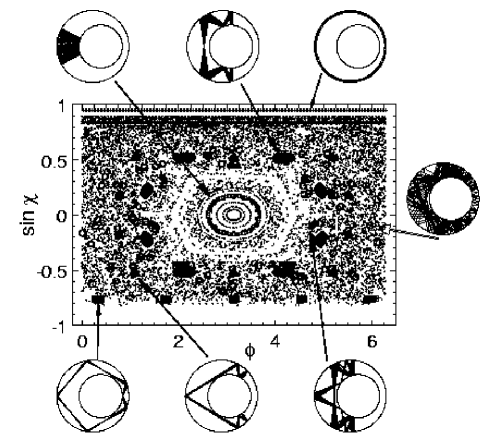
FIG. 5.: Poincaré SOS taken at the outer boundary for the hard-wall annular billiard ($R_{2}=0.6,\delta=0.22$). Trajectories are bounded to the annular region, no optical properties of the system are yet included. Typical regular and chaotic trajectories are shown both in real and phase space.

For optical systems, both the outer and inner boundary become permeable. Leakage at the outer boundary occurs for $-1/n<\sin\chi<1/n$. In the simplest qualitative picture, starting with the hard-wall system, we will assume those rays to leave the cavity (thus simplifying Fresnel’s laws (1) to a stepwise function). The corresponding trajectories are assumed to not exist in an optical cavity. If one is interested in how the intensity of a certain trajectory decreases, Fresnel’s laws can easily be taken into account accurately, leading to the model of a Fresnel billiard [6, 24, 37].

However, the description of the refractively opened inner boundary turns out to be rather complicated. There, all rays remain in the billiard, causing a tremendous increase of the number of rays upon partial reflection. Another crucial difference is that now new trajectories arise, namely those crossing the inner disk. We model this situation by introducing the model of the “refractive billiard”: Whenever total internal reflection is violated at the inner boundary, the ray enters the inner disk according to Snell’s law with full intensity, such that now ray splitting occurs. Otherwise, the ray is specularly reflected and stays in the annulus. This corresponds again to a stepwise simplification of Fresnel’s laws. Note that the hard-wall billiard is in fact a realization of constant reflection coefficient $R^{\rm TM/TE}=1$. The real situation is found in between the stepwise and constant approximations and, depending on the refractive indices chosen, results from both limits are needed in order to understand the resonant modes found in the wave picture, see Sec. IV.

We complete our refractive-billiard model by first assuming specular reflection at the outer boundary, and discuss outer-boundary losses subsequently as outlined above. Results are shown in Figs. 6 and 7 for the same geometry as in Fig. 5 [38], and two different combinations of refractive indices. In Fig. 6, the annular index $n_{1}$ is highest, allowing for total internal reflection at both boundaries. In the limit $n_{1}\to\infty$ we would recover the phase space of the hard-wall billiard, Fig. 5. For moderate $n_{1}=3$ ($n_{0}=n_{2}=1$) as in Fig. 6 we are, however, away from this limit: most of the regular trajectories of the hard-wall system are gone and, in turn, new regular orbits passing through the inner disk appear.

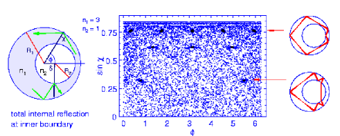
FIG. 6.: Poincaré SOS taken at the outer boundary for the refractive billiard with $n_{0}=1,n_{1}=3,n_{2}=1$ and the same geometry as in Fig. 5. The hard-wall condition of Fig. 5 is kept at the outer boundary, but replaced at the inner one by the condition of total internal reflection. If it is not fulfilled the ray will penetrate the inner disk, giving rise to a restructured phase space and new regular orbits as the one on the lower right.

The situation changes once more for $n_{0}<n_{1}<n_{2}$, because then total internal reflection at the inner boundary is never possible (again, we base our discussion on rays entering from the annulus), and all rays hitting the inner boundary will enter. Furthermore, they will leave the inner disk upon the next reflection according to the principle of reversibility of the light path. Note, however, that confinement by total internal reflection in the inner disk is well possible. From our discussion in Sec. II we know that these orbits will and can only be whispering gallery modes (WGMs). To anticipate results of the next section, those modes do exist and leave their signature as very sharp peaks in the delay time.

In Fig. 7 an example of the phase space is given, showing yet another structure owing to the change in the refractive indices. For the regular orbits shown at the right, we expect only the upper one to survive the (optical) opening of the outer boundary as long as $n_{0}/n_{1}\geq 3.2$. The lower orbit hits the outer boundary perpendicular ($\chi=0$) at least in some points, and can therefore only be confined by hard walls.

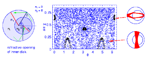
FIG. 7.: Poincaré SOS for the refractive billiard with $n_{0}=1,n_{1}=3,n_{2}=6$ and the same geometry as in Fig. 5. Rays in the annulus that hit the inner boundary will penetrate it. Note the existence of whispering gallery modes in the inner disk (confined by total internal reflection) not visible in this SOS.

B Wave picture: Maxwell’s equations and $S$-matrix approach

Generalizing the wave picture approaches presented in Sec. II for the dielectric disk to the annular billiard requires essentially to consider another, off-centered circular boundary at which the matching conditions resulting from Maxwell’s equations have to be fulfilled as well. An eccentric inclusion lowers the rotational symmetry of the system to axial reflection invariance about the symmetry axis of the system. Consequently, angular momentum is not conserved, and the $S$-matrix of the compound system cannot be diagonal in the general case.

Maxwell’s equations can be solved analytically in the concentric case ($R_{2}>0$), and resonant states with complex wave number are obtained as zeros of the expression

$$n_{1}J_{m}(k_{2}R_{2}){H_{m}^{(1)}}^{\prime}(k_{0}R_{1})\times$$ (11)

$$\times\left[{H_{m}^{(2)}}^{\prime}(k_{1}R_{2})H_{m}^{(1)}(k_{1}R_{1})-{H_{m}^{(1)}}^{\prime}(k_{1}R_{2})H_{m}^{(2)}(k_{1}R_{1})\right]$$

$$- n_{1}^{2}J_{m}(k_{2}R_{2})H_{m}^{(1)}(k_{0}R_{1})\times$$ (13)

$$\times\left[{H_{m}^{(2)}}^{\prime}(k_{1}R_{2}){H_{m}^{(1)}}^{\prime}(k_{1}R_{1})-{H_{m}^{(1)}}^{\prime}(k_{1}R_{2}){H_{m}^{(2)}}^{\prime}(k_{1}R_{1})\right]$$

$$- n_{2}J^{\prime}_{m}(k_{2}R_{2}){H_{m}^{(1)}}^{\prime}(k_{0}R_{1})\times$$ (15)

$$\times\left[H_{m}^{(2)}(k_{1}R_{2})H_{m}^{(1)}(k_{1}R_{1})-H_{m}^{(1)}(k_{1}R_{2})H_{m}^{(2)}(k_{1}R_{1})\right]$$

$$+ n_{1}n_{2}J^{\prime}_{m}(k_{2}R_{2})H_{m}^{(1)}(k_{0}R_{1})\times$$ (17)

$$\times\left[H_{m}^{(2)}(k_{1}R_{2}){H_{m}^{(1)}}^{\prime}(k_{1}R_{1})-H_{m}^{(1)}(k_{1}R_{2}){H_{m}^{(2)}}^{\prime}(k_{1}R_{1})\right]$$

for TM polarized light. Note that Eq. (11) reduces to Eq. (6) for $n_{1}=n_{2}$ when the annular billiard is reduced to a disk.

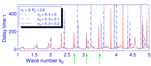
FIG. 8.: Resonance peaks for increasing displacement $\delta$ in comparison with the concentric case (dotted) for $n_{2}>n_{1}$. Here, whispering gallery modes of the outer disk are shifted to the left due to an increase of the effective refractive index. However, other modes are affected in a different way, as for example the resonances marked by arrows.

In order to investigate the eccentric case, we focus on the $S$-matrix method. The derivation of the $S$-matrix for the eccentric annular billiard is outlined in the appendix. As discussed in Sec. II the information on resonance position and width is contained both in the complex wave vector that solves the resonance equation deduced from Maxwell’s equations and in the delay-time plot $\tau(k)$. This is illustrated in the inset of Fig. 4(a) where the resonance positions and widths found from $\tau(k)$ are compared with the numerically exact solutions of Eq. (11) for concentric geometries. The delay-time plot in Fig. 4(a) reveals a systematic deviation of the first few resonance positions to the right (left), if the refractive index of the inner disk is lower (higher) than that in the annulus. However, the deviation from the concentric case is rather small. It suggests that the low-lying resonances in the (concentric) annular geometry are very similar to the WGMs of the dielectric disk and mainly localized at the outer boundary. However, the resonant wave function does experience the change of the refractive index in the inner disk as indicated by the shift of the resonance position. The direction of the shift is most easily seen when thinking in terms of an effective refractive index $n_{\rm eff}$,

$$n_{\rm eff}\stackrel{{\scriptstyle\rm def}}{{=}}\left(1-\frac{R_{2}^{2}}{R_{1}^{2}}\right)n_{1}+\frac{R_{2}^{2}}{R_{1}^{2}}n_{2}\>.$$ (18)

An inner disk of lower refractive implies $n_{\rm eff}<n_{1}$ and a larger spacing between the resonances. This is easily understood when considering an eigenvalue $nk=$const. of the (closed) dielectric disk. Obtaining the same constant value for a smaller $n$ requires a higher $k$. In contrast, an inner disk of higher refractive index reduces the spacing between the resonances. This effect is strongest for resonances of high radial quantum number $\rho$ and small angular momentum quantum number $m$, since they rather extend to the inner regions of the disk or the annular billiard. (In terms of the ray picture, they correspond to smaller angles of incidence, leading to the same conclusion.) Accordingly, the effect reduces for increasing $m$ and eventually vanishes if the inner disk is not seen any more [39]. In Fig. 4(a) resonances are marked by arrows that exist only if the refractive index of the inner disk is highest. One corresponding wave pattern, together with a ray analogue, is shown in Fig. 4(b). It reveals that the “double WGM” structure results from a star-like trajectory.

In Fig. 8 we consider the same refractive indices (i.e. $n_{1}=3,n_{2}=4$) and shift now the inner disk off the centre. The “double WGMs” (again marked by arrows) are affected in a way different from the “conventional” WGMs. First of all, the systematic shift of the latter can again be understood in terms of the effective refractive index. The impact of an off-centered (inner) disk is enhanced because in the constricted region it acts like a concentric disk with larger radius $R_{2}^{\rm eff}>R_{2}$. Note that the resonances marked by arrows in Fig. 8 change their character from “double WGMs” in the concentric and slightly eccentric cases to “generalized” WGMs similar to the one shown in the right panel of Fig. 9 if the symmetry breaking caused by the off-centered inner disk becomes too strong.

IV Ray-wave-correspondence for the annular billiard

In the previous sections we already referred to the ray-wave correspondence in optical systems and gave several examples which were mainly based on WG modes, and the concentric annular billiard. In this section, we first continue with WGMs and show how they can be specifically influenced by choosing appropriate materials. However, ray-wave correspondence holds for far more interesting trajectories, and we will give illustrative examples how closed-billiard trajectories are recovered in the open system using real and phase space portraits.

A Classes of whispering gallery modes in annular systems

In Sec. II we introduced the concept of the effective potential as a wave-picture method when we established the analogy between Helmholtz and Schrödinger equations. The generalization of this concept to the annular billiard is straightforward and (in the concentric case) essentially given by the superposition of two disks, see Eq. (3). The result is schematically shown in Fig. 9. Again, we have to distinguish two cases: In Fig. 9(a), the refractive index $n_{1}$ in the annulus is highest, whereas in Fig. 9(b) the optical density increases towards the inner disk. Consequently, in the first case, Fig. 9(a), the potential well coincides with the annular region: Rays in between the two disks can be totally reflected at either boundary as illustrated in the lower panels.

The situation is different when the refractive index $n_{2}$ of the inner disk is highest [Fig. 9(b)]. The well extends now beyond the inner boundary to values $r<R_{2}$ indicating that the inner disk may support annular WGMs in the constricted region, see the lower panels. This is consistent with the ray picture interpretation stating that each ray in the annulus that hits the inner boundary will enter the inner disk. However, because of the double-well structure of the effective potential this case is even richer: There are modes that mainly live in one of the two wells, corresponding to WGMs of the inner and outer disk, respectively. The height of the separating barriers depends on the wave number, the quantum number $m$, the geometry, and in particular on the ratio of the refractive indices that can be used to tune the height of the barrier (note that at the same time the depths of the minima are changed).

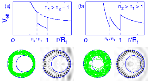
FIG. 9.: Effective potential for the annular billiard for two different sets of refractive indices ($n_{0}$=1). In the lower panels corresponding examples of ray trajectories (left) and wave functions (right) are shown. The similarity of these resonances to whispering gallery modes suggest their classification as “generalized” WGMs.

B Towards closed systems

Varying the refractive index of an optical system allows one to describe the transition between closed and open, optical, systems as mentioned earlier. To illustrate this fact we increase the refractive index of the annular region that we assume to be embedded in vacuum ($n_{0}=n_{2}=1$, wave vector $k_{0}=k_{2}$). The length spectrum, or Fourier transform, of the delay time $\tau(k_{0})$ is shown in Fig. 10(a) for refractive indices $n_{1}=3$ and $n_{1}=6$ (dashed and full line, respectively). The Fourier analysis is performed in the spirit of trace formulas that provide a semiclassical interpretation of quantum-mechanical results in terms of classical periodic orbits for quantum billiards. The quantitative extension of this approach to optical systems will require further discussion. Here, we are only interested in a qualitative interpretation.

We have divided the optical length that results from the Fourier transformation by $n_{1}$ in order to compare both spectra in terms of geometrical lengths $L$. The peaks in both spectra are rather broad and correspond roughly to the circumference of the bigger disk (and higher harmonics) which indeed is a typical trajectory length in this geometry not only for WGMs, but also for the trajectory examples shown Figs. 5 and 11 (trajectory parts in the inner disk will contribute a length that has to be corrected by a factor $n_{2}/n_{1}$). However, the length spectrum for $n_{1}=6$ shows an additional peak (marked by the arrow) at higher $L$. A ray trajectory of suitable length is shown in Fig. 10(b). The Poincaré fingerprint of this orbit, see Fig. 5, possesses regular islands at $\sin\chi=0$, where in the simplest interpretation refractive escape will occur, independent on the refractive index! That modes of this type are found for sufficiently large $n_{1}$, indicates that we have to refine our interpretation. For example, we can discuss the Fresnel reflection coefficient $R_{\perp}$ at normal incidence, $R_{\perp}=(n_{0}-n_{1})^{2}/(n_{0}+n_{1})^{2}$ that increases as $n_{1}$ is increased, reaching the value one in the limit $n_{1}\to\infty$, in accordance with the picture of complete internal reflection. This explains the observed behaviour and we present more examples of “sophisticated” ray-wave, or classical-quantum, correspondence in the next paragraph.

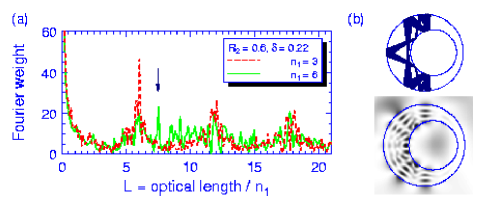
FIG. 10.: (a) Fourier transform of the delay time $\tau(k_{0})$ for the annular billiard geometry $R_{2}=0.6,\delta=0.22$ and two refractive index combinations, $n_{0}=n_{2}=1$, $n_{1}=3$ (dashed line), and $n_{1}=6$ (full line). The appearance of a new peak at larger geometric length is clearly visible. A suitable (quasi-) periodic orbit candidate together with a resonant state is shown in (b).

C Correspondence in real and phase space

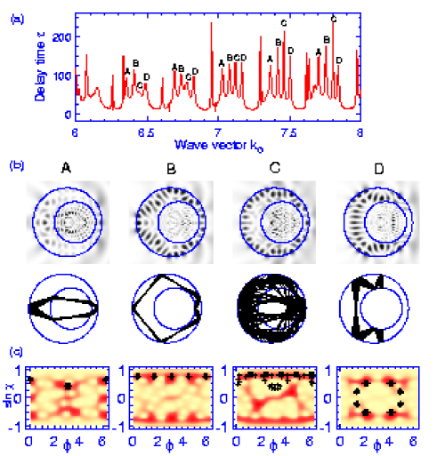
FIG. 11.: (a) Delay time $\tau(k_{0})$ for the annular billiard geometry as in Figs. 5 and 10 and $n_{1}=3,n_{2}=6$. The structure is dominated by groups of four resonances labelled A, B, C, D. The resonance at $k_{0}\approx 6.251$ is the one shown in Fig. 1(b). The four resonances of the second group ($6.6<k_{0}<6.9$) are shown in (b) together with a ray trajectory representative. In part (c), rays (crosses) and waves (intensity plot, high intensity in dark regions) are compared in phase space in terms of their Poincaré and Husimi representation, respectively.

In Fig. 11(a) we show a typical delay-time plot $\tau(k_{0})$ for the annular billiard with the same geometry as before and refractive indices $n_{1}=3,n_{2}=6$. We investigate low-lying resonances that show a characteristic grouping of four resonances (marked by A, B, C, D) over several periods. The corresponding wave patterns, together with suggestions for ray analogues, are shown in Fig. 11(b) for each resonance. We have mainly chosen regular orbits as candidates because of the regular structure of the delay-time plot. Neighbouring resonances of the same kind (i.e., the same letter) indeed differ by one in the number of nodes[40]. Note that the ray representatives stem from both the hard-wall and the refractive billiard simulation, see Figs. 5 and 7.

In Fig. 11(c) we computed the Husimi function [17, 21, 41] for each of the wave functions [42], and marked the rays by crosses in the corresponding Poincaré SOS such that we can directly compare the phase space presentations of waves and rays. The coincidence between regular islands and high-probability regions (dark) of the Husimi function appears satisfying on first sight. However, closer inspection reveals differences in the details. For example, Husimi “islands” are shifted away from regular islands as in the case of resonance D, with the corresponding real space modifications [Fig. 11(b)] clearly visible as well. One possible explanation might be provided by the Goos-Hänchen effect that causes a lateral shift of the reflected ray for angles of incidence around and greater than the critical angle [30, 31], thereby effectively changing the angle of incidence. Furthermore, we point out that the ray trajectory for resonance D is known from the hard-wall system. The qualitative similarity to the corresponding resonant wave pattern is remarkable, and one might think of the differences as in order to meet the new interference requirements caused by the optical opening of the inner disk. This gives yet another example of the predictive power of the simple ray model when only the qualitative character of the resonances is of interest and importance. On the other hand, it proves to be essential to consult wave methods when one is interested in details.

V Conclusions

To conclude, we have investigated the ray and wave properties of composite optical systems by applying methods known from the classical and quantum theory of mixed dynamical systems. Using the optical annular billiard as an example, we have shown this concept to be very fruitful. This means in particular that already the simple ray model provides a good qualitative understanding of the system properties, even for small wave numbers below $nkR\approx$ 30. However, care must be taken when quantitative results are required, or the classical (ray) phase space is directly translated into expected wave patterns: We find regular orbits associated with regular islands in phase space to be the dominant class of resonant wave patterns, and suppression of wave functions hosted by the chaotic part of the phase space. The dependence of this behaviour on the size of the wave number (i.e. $1/\hbar$) remains an interesting topic for future work.

One remark is due concerning the refractive indices employed in the calculations. The index $n=3$ often used here is higher than that of water (1.33) or glass (around 1.5 up to 1.8) but is easily reached in semiconductor compounds where typically $n=3.3$. An index $n=6$ seems to be presently out of reach, which, however, does not affect the conclusions drawn here.

Summerizing, ray picture results may serve as a guide in the investigation of wave properties of optical systems, even away from the ray limit $k\to\infty$. For the annular billiard as an example of a compound cavity system we demonstrated that the dominant resonant wave patterns can be seen as originating from the regular orbits of both the hard-wall and the refractive billiard. This knowledge can be more generally used, e.g., in the construction of microlasers with designed properties. Knowing the potential reflection points and high-intensity regions of modes from simple ray-based considerations allows one to design microcavities with custemized properties. Predictions can be made concerning, e.g., the effective coupling between and into cavities or how to efficiently pump lasing systems. In turn, one can think of cavity shapes designed according to the technical requirements. The application of the ray-wave correspondence in sophisticated optical (compound) systems therefore may provide a powerful tool for future optical communication technologies.

Optical cavities represent interesting model systems for quantum-chaos motivated studies. We successfully applied the $S$-matrix approach to gain spectral information, and qualitatively discussed its periodic-orbit interpretation [44]. The development of quantitative semiclassical theories in the spirit of the Weyl and the trace formulas remains an open subject, in particular for compound systems consisting of more than one region with fixed refractive index like the annular billiard.

A $S$-matrix for the annular billiard

We will generalize the ideas developed in Sec. II C to the dielectric annular billiard in order to determine the $S$-matrix for the eccentric annular billiard. This problem can be divided into the scattering problem at the outer boundary (between refractive indices $n_{0}$ and $n_{1}$) and that at the inner boundary (between indices $n_{1}$ and $n_{2}$). Although the scattering at a dielectric disk was solved in Sec. II C, the situation we are confronted with here is more complicated: the two disks lay one in the other, and their centres will in general not coincide.

We will begin with the scattering problem at the inner boundary and express the $S$-matrix $S^{i}$ of the dielectric disk with respect to a coordinate system with origin displaced from the centre of the inner disk. This implies that $S^{i}$ is not diagonal. From Sec. II C we already know the (diagonal) $S$-matrix $S^{ic}$ of the inner disk in primed coordinates (see Fig. 1), Eq. (7). We will now derive the relation between $S^{ic}$ and $S^{i}$.

To this end we write the ansatz for the wave function in the annulus in primed coordinates, $\vec{r^{\prime}}=\vec{r}-\vec{\delta}$, with $\vec{\delta}$ being the vector from the centre of the large disk to the centre of the smaller disk, as

$$\Psi^{1c}(\vec{r}-\vec{\delta}) = \sum_{l=-\infty}^{\infty}a^{c}_{l}\left[H_{l}^{(2)}(k_{1}|\vec{r}-\vec{\delta}|)e^{il\phi}\right.$$ (A2)

$$\left.+\sum_{l^{\prime}=-\infty}^{\infty}S^{ic}_{ll}H_{l^{\prime}}^{(2)}(k_{1}|\vec{r}-\vec{\delta}|)e^{il^{\prime}\phi}\right]\>,$$

where the coefficients $a^{c}_{l}$ are to be chosen to yield the desired kind of incident wave. We use the addition theorem for Bessel functions $Z_{m}\in\{J_{m},Y_{m},H_{m}^{(1)},H_{m}^{(2)}\}$ [43] to relate the arguments $wr$ to $wr^{\prime}$ ($w$ is a constant factor, and we assume$R_{2}>\delta$), see Fig. 12,

$$Z_{m}(wr^{\prime})e^{im\phi}=\sum_{k=-\infty}^{\infty}J_{k}(w\delta)Z_{m+k}(wr)e^{i(m+k)\phi}\>.$$ (A3)

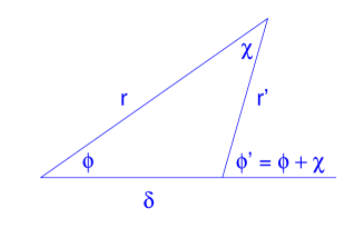
FIG. 12.: Addition theorem for Bessel functions.

Inserting this into Eq. (A2), we obtain the expression

$$\widetilde{\Psi}^{1} = \sum_{l=-\infty}^{\infty}\sum_{k=-\infty}^{\infty}a^{c}_{l}\left[H_{l+k}^{(2)}(k_{1}r)+S^{ic}_{ll}H_{l+k}^{(1)}(k_{1}r)\right]\times$$ (A5)

$$\times J_{k}(k_{1}\delta)\>e^{i(l+k)\phi}$$

for the wave function in the annulus, now expressed with respect to the centre of the larger disk, i.e., in unprimed coordinates. We specify the coefficients $a^{c}_{l}$ by the requirement that the amplitude of an incident wave with angular momentum $m$ shall be normalized to one in unprimed coordinates,

$\displaystyle\sum_{l=-\infty}^{\infty}\sum_{k=-\infty}^{\infty}a^{c}_{l}H_{l+k}^{(2)}(k_{1}r)J_{k}(k_{1}\delta)\>e^{i(l+k)\phi}\equiv H_{m}^{(2)}(k_{1}r)\>e^{im\phi}\>.$

With $\mu\equiv l+k$, and $\sum_{k}J_{m-(\mu-k)}J_{k}=\delta_{m\mu}$ we find that choosing

$${}^{m}a^{c}_{l}=J_{m-l}(k_{1}\delta)\quad\forall\>\,l$$ (A6)

provides a suitable set of coefficients for a given $m$. Accordingly, we write

$$\widetilde{\Psi}^{1} = \sum_{m=-\infty}^{\infty}\Bigg{\{}\sum_{\mu,k=-\infty}^{\infty}\left[\delta_{m\mu}H_{\mu}^{(2)}(k_{1}r)e^{i\mu\phi}\right.$$ (A8)

$$\left.+J_{m-(\mu-k)}(k_{1}\delta)S^{ic}_{(\mu-k)(\mu-k)}J_{k}(k_{1}\delta)H_{\mu}^{(1)}(k_{1}r)e^{i\mu\phi}\right]\Bigg{\}}$$

$$\equiv \sum_{m=-\infty}^{\infty}\left\{H_{m}^{(2)}(k_{1}r)e^{im\phi}+\sum_{\mu=-\infty}^{\infty}S^{i}_{m\mu}H_{\mu}^{(1)}(k_{1}r)e^{i\mu\phi}\right\}$$ (A9)

where we have read off the scattering matrix $S^{i}$ of the inner disk with respect to the centre of the outer disk,

$$S^{i}_{m\mu}\stackrel{{\scriptstyle\rm def}}{{=}}\sum_{k=\infty}^{\infty}J_{m-(\mu-k)}(k_{1}\delta)S^{ic}_{(\mu-k)(\mu-k)}J_{k}(k_{1}\delta)\>.$$ (A10)

The structure of this equation suggests a notation in terms of a transformation matrix $U$, namely $S^{i}=U^{-1}S^{ic}U$, that describes the change in the origin of the coordinate system. We find $U_{l^{\prime}l}=J_{l^{\prime}-l}$ and $U^{-1}_{l^{\prime}l}=J_{l-l^{\prime}}$.

The scattering matrix $S^{i}$ allows us to describe the scattering at an off-centred disk, and we can now formulate the scattering problem of the annular billiard in the spirit of Sec. II C. Accordingly, we start with an ansatz for the wave function $\Psi^{0}$ outside the annular system ($|\vec{r}|>R_{1}$, using polar coordinates) of the form

$$\Psi^{0}(\vec{r}) = \sum_{M=-\infty}^{\infty}\Psi^{0}_{M}(\vec{r})$$ (A11)

$$= \sum_{M=-\infty}^{\infty}\left[\Psi_{M}^{-}(k_{0}\vec{r})+\sum_{M^{\prime}=-\infty}^{\infty}S_{MM^{\prime}}\Psi_{M^{\prime}}^{+}(k_{0}\vec{r})\right]\>,$$ (A12)

where we have introduced the scattering matrix $S$ of the (compound) system and the definitions

$$\Psi_{M}^{-}(k_{0}\vec{r}) = H_{M}^{(2)}(k_{0}r)e^{iM\phi}\>,$$ (A13)

$$\Psi_{M}^{+}(k_{0}\vec{r}) = H_{M}^{(1)}(k_{0}r)e^{iM\phi}\>,$$ (A14)

for incoming and outgoing waves outside the disk. Note that we have used the freedom in fixing one of the amplitudes.

Similarly, we write for the wave function $\Psi^{1}$ in the annular region

$$\Psi^{1}(\vec{r})=\sum_{l=-\infty}^{\infty}a_{l}\left[\Psi_{l}^{-}(k_{1}\vec{r})+\sum_{l^{\prime}=-\infty}^{\infty}S^{i}_{ll^{\prime}}\Psi_{l^{\prime}}^{+}(k_{1}\vec{r})\right]\>,$$ (A15)

with the amplitudes $a_{l}$, the abbreviations as in Eqs. (A13, A14), and $S^{i}$ from Eq. (A10).

Now, we determine $S$ from the matching conditions, introduce the notation of capital letters for functions of argument $k_{0}r$, and reserve lower case characters for the argument $k_{1}r$. Given an incident wave of angular momentum $M$, wave function matching for each angular momentum $L$ of the scattered waves yields

$$H_{M}^{(2)}e^{iM\phi}\delta_{ML}+S_{ML}H_{L}^{(1)}e^{iL\phi}$$ (A16)

$$\quad\quad\quad=a_{L}^{(M)}h_{L}^{(2)}e^{iL\phi}+\sum_{l=-\infty}^{\infty}a_{l}^{(M)}S^{i}_{lL}h_{L}^{(1)}e^{iL\phi}\>,$$ (A17)

where the amplitudes $a_{j}^{(M)}$ are coefficients associated with an incoming function of angular momentum $M$, namely $H_{M}^{(2)}$. Since this has to hold for all $M$, and at fixed $M$ for all $L$, we write this as a matrix equation

$$\langle{}^{(M)}H^{(2)}|+\langle S^{(M)}|H^{(1)}=\langle a^{(M)}|\left(h^{(2)}+S^{i}h^{(1)}\right)\>,$$ (A18)

where $S^{i}$ is a matrix, $h^{(2)}$ and $h^{(1)}$ are diagonal matrices, $h^{(1,2)}_{lj}=h^{(1,2)}_{l}\delta_{lj}$, and we adopt the bra-notation for quantities that, at fixed $M$, are transposed vectors and gain matrix character once $M$ is varied. With this notation we immediately write the matching condition for the derivatives as

$$k_{0}\left(\langle{}^{(M)}{H}^{(2)^{\prime}}|+\langle S^{(M)}|{H}^{(1)^{\prime}}\right)\$$ (A19)

$$\quad\quad\quad=\langle a^{(M)}|k_{1}\left({h^{(2)}}^{\prime}+S^{i}{h^{(1)}}^{\prime}\right)\>.$$ (A20)

From Eq. (A18) we find after substituting $F\equiv h^{(2)}+S^{i}h^{(1)}$ that

$\displaystyle\langle a^{(M)}|=\left(\langle{}^{(M)}H^{(2)}|+\langle S^{(M)}|H^{(1)}\right)\,F^{-1}\>.$

Introducing furthermore $F^{\prime}={h^{\prime}}^{(2)}+S^{i}{h^{\prime}}^{(1)}$ and $W=F^{-1}F^{\prime}$, we write the $S$-matrix solution of the problem as

$\displaystyle S=\left(k_{1}\,H^{(2)}\,W-k_{0}\,{H^{\prime}}^{(2)}\right)\left(k_{0}\,{H^{\prime}}^{(1)}-k_{1}\,H^{(1)}\,W\right)^{-1}\>.$

This last equation allows us to apply the Wigner-delay-time approach to resonances, cf. Sec. II C, and we used this method to study resonances of the optical annular billiard, cf. Secs. III and IV.

We complete the discussion here with some comments on the wave functions. We have not yet given the wave function in the inner disk. The ansatz is a sum over Bessel functions,

$\displaystyle\Psi^{2c}(\vec{r^{\prime}})=\sum_{l=-\infty}^{\infty}b^{c}_{l}J_{l}(k_{2}r^{\prime})e^{il\phi^{\prime}}\>,$

where we adopted primed coordinates for convenience. The coefficients $b_{l}$ are found from matching with the wave function in the annulus at the inner boundary. To this end we have to rewrite the annular wave function (A15) in terms of primed coordinates by applying the addition theorem (A3) for Bessel functions. After straightforward algebra we find

$\displaystyle\Psi^{1c}(\vec{r^{\prime}})=\sum_{l=-\infty}^{\infty}a^{c}_{l}\left[H_{l}^{(2)}(k_{1}r^{\prime})+S^{ic}_{ll}H_{l}^{(1)}(k_{1}r^{\prime})\right]e^{il\phi^{\prime}}\>,$

where the coefficients $a_{l}^{c}$ are related to the $a_{l}$ by $a_{l}^{c}=\sum_{l^{\prime}=-\infty}^{\infty}a_{l^{\prime}}J_{l^{\prime}-l}$.

Another remark is in order concerning the validity of the addition-theorem-based expansion of the Bessel function when changing between primed and unprimed coordinates. Expansion of the annular wave function in primed coordinates fails near the outer boundary where $|\vec{r^{\prime}}|>R_{1}-R_{2}-\delta$. Similarly, expanding the annular wave function in unprimed coordinates does not work near the inner boundary where $|\vec{r}|<R_{2}+\delta$. The reason for this behaviour is that angular momentum is not conserved in the eccentric annular billiard, and the expansion breaks down at radii where waves explore this symmetry-breaking region because the corresponding interface boundaries are hit.

REFERENCES

- [1] Present address: Department of Physics, Duke University, Box 90305, Durham, NC 27708-0305
- [2] H. J. Stöckmann and J. Stein, Phys. Rev. Lett. 64, 2215 (1990).
- [3] H.-D. Gräf et al., Phys. Rev. Lett. 69, 1296 (1992); H. Alt et al., Phys. Rev. Lett. 79, 1026 (1996).
- [4] A. Andersen et al., Phys. Rev. E 63, 066204 (2001).
- [5] J. U. Nöckel, PhD Thesis, Yale University, 1997.
- [6] J. U. Nöckel and A. D. Stone, Nature 385, 45 (1997).
- [7] J. A. Lock et al., Appl. Optics 37, 1527 (1998).
- [8] P. B. Wilkinson et al., Phys. Rev. Lett. 86, 5466 (2001).
- [9] S.-B. Lee et al., Phys. Rev. Lett. 88, 033903 (2002).
- [10] V. Doya et al., Phys. Rev. Lett. 88, 014102 (2002).
- [11] S. Chang et al., J. Opt. Soc. Am. B 17, 1828 (2000).
- [12] S. A. Backes et al., J. Vac. Sci. Technol. B 16, 3817 (1998).
- [13] C. Gmachl et al., Science 280, 1556 (1998).
- [14] J. D. Jackson: Classical Electrodynamics (John Wiley & Sons, New York, 1975).
- [15] H.-J. Stöckmann: Quantum Chaos (Cambridge University Press, 1999).
- [16] O. Bohigas, D. Boosé, R. Egydio de Carvalho, and V. Marvulle, Nucl. Phys. A560, 197 (1993).
- [17] S. D. Frischat and E. Doron, Phys. Rev. Lett. 75, 3661 (1995); Phys. Rev. E 57, 1421 (1998).
- [18] C. Dembowski et al., Phys. Rev. Lett. 84, 867 (2000).
- [19] A. Kohler and R. Blümel, Ann. Phys. 267, 249 (1998); Phys. Lett. A238, 271 (1998).
- [20] For such open annular billiards questions concerning the doublet-splitting addressed in [16, 17] are not of relevance because the splitting it masked by resonance broadening.
- [21] G. Hackenbroich and J.-U. Nöckel, Europhys. Lett. 39, 371 (1997).
- [22] G. Gouesbet, S. Meunier-Guttin-Cluzel, and G. Gréhan, Opt. Comm. 201, 223 (2002).
- [23] J.U. Nöckel and A.D. Stone, in: Optical Processes in Microcavities (Editors: R.K. Chang, A.J. Campillo), World Scientific Publishers (1996).
- [24] M. Hentschel and M. Vojta, Opt. Lett. 26, 1764 (2001).
- [25] The vector character of light requires to distinguish between two polarizations. In our planar systems, either the transverse magnetic (TM) or electric (TE) field can lie in the system plane.
- [26] G. Gouesbet, S. Meunier-Guttin-Cluzel, and G. Gréhan, Phys. Rev. E 65, 016212 (2001).
- [27] S. G. Lipson, H. Lispon, and D. S. Tannhauser: Optical Physics (Cambridge University Press, 1995).
- [28] The first derivative in the first term can be eliminated by a substitution .
- [29] M. Hentschel and J. U. Nöckel, in: Quantum Optics of Small Structures (Editors: D. Lenstra, T. D. Visser, and K. A. H. van Leeuwen), Edita KNAW (2000); arXiv:physics/0203064.
- [30] M. Hentschel and H. Schomerus, Phys. Rev. E 65, 045603 R (2002).
- [31] F. Goos and H. Hänchen, Ann. Phys. (Leipzig) 1, 333 (1947); H. M. Lai, F. C. Cheng, and W. K. Tang, J. Opt. Soc. Am. A 3, 550 (1986); H. K. V. Lotsch, Optik (Stuttgart) 32, 116 (1970), 189 (1970), 299 (1971), 553 (1971).
- [32] E. Doron and U. Smilansky, Nonlinearity 5, 1055 (1992).
- [33] J. R. Taylor: Scattering Theory (Robert E. Krieger Publishing Company, Malabar/Florida, 1983).
- [34] U. Smilansky in: Mesoscopic Quantum Physics, Les Houches, Session LXI 1994 (Editors: E. Akkermans, G. Montambaux, J. L. Pichard, and J. Zinn-Justin).
- [35] R. G. Newton: Scattering Theory of Waves and Particles (Springer, New York, 1982); Y. V. Fyodorov and H.-J. Sommers, J. Math. Phys. 38, 1918 (1997).
- [36] For microlaser operation, resonances of intermediate width are of particular interest: For too broad resonances leakage ceases the crossing of the lasing threshold, whereas very narrow resonances will fail to provide sufficient output power.
- [37] M. V. Berry, Eur. J. Phys. 2, 91 (1981).
- [38] The geometry parameters mainly studied here were chosen because of the particularly interesting phase space structure. Generalization of the results to other geometries is straightforward.
- [39] This applies to the families of WGMs with small and depends on the size of the inner disk.
- [40] Having in mind the ratio of regular to chaotic regions in the corresponding Poincaré SOS, Fig. 5, regular modes appear to be over-represented for the (small) wave numbers considered here. One might even argue that smaller regular islands cannot be resolved. However, similar effects have been observed before, see, e.g., R. Ketzmerick, L. Hufnagel, F. Steinbach, and M. Weiss, Phys. Rev. Lett. 85, 1214 (2000).
- [41] B. Crespi, G. Perez, and S.-J. Chang, Phys. Rev. E 47, 986 (11993); A. M. Ozorio de Almeida: Hamiltonian Systems: Chaos and Quantization (Cambridge University Press, 1998).
- [42] We used the expressions valid for a refractive index boundary, see M. Hentschel, H. Schomerus, R. Schubert, submitted to Phys. Rev. Lett.; R. Schubert, in preparation.
- [43] I. S. Gradshteyn and I. M. Ryzhik: Table of integrals, series, and products (Editor: A. Jeffrey), Academic Press, San Diego (1994).
- [44] M. Hentschel, PhD Thesis, Technical University of Dresden, 2001.