The Determination of Microscopic Surface Tension of Liquids with a Curved Interphase Boundary by Means of Positron Spectroscopy

Abstract:

The method for determination the microscopic surface tension $\sigma(R)$ of nanobubbles is developed based on the new elaboration of the positronium bubble model. In contrast to existing structureless Ps bubble models, our version contains experimentally known molecular characteristics of liquids. The relationship, similar to Tolman’s equation, between $\sigma(R)$ and the radius $R$ of the Ps bubble is derived on a microscopic basis. Numerical values for $\sigma(R)$ are determined for a large number of liquids and liquified gases. The results are in agreement with the theoretical expectations and independent evaluations, available in literature.

Keywords: surface tension, positronium, nanobubbles, interphase boundary, cavity formation.

The author to whom correspondence should be sent:

Sergey Vsevolodovich Stepanov
Institute of Theoretical and Experimental Physics
Bolshaya Cheremushkinskaya 25
Moscow, 117218, Russia
e-mail: stepanov@vxitep.itep.ru
phone/fax: (095)125-7124; 129-9751

I Introduction

More than one hundred years ago Willard Gibbs in the frameworks of thermodynamic approach established that if the surface of a liquid is curved, the surface tension coefficient $\sigma$ gets a function of curvature $1/r$ of the interphase boundary. Investigations of Gibbs were extended by Tolman [1] and others [2, 3]. It was found that behavior of $\sigma(r)$ for droplets and bubbles is different. For droplets $\sigma(r)$ is approximately described by Tolman’s equation:

$$\sigma(r)=\frac{\sigma_{\infty}}{1+2\Delta/r},$$

where $\sigma_{\infty}$ is the tension for a plane surface and the ”Tolman distance” $\Delta$ is equal to the distance between the equimolecular dividing surface and the surface of tension.

In case of bubbles $\sigma(r)$ may pass through a maximum [3] and than goes to zero, but in both cases at small $r$  $\sigma(r)\propto r$ [4]. Special additional assumptions are made concerning the behavior of the Tolman parameter $\Delta$ as a function of $r$ [3].

However applicability of the thermodynamic approach to very small systems such as liquid droplets in the gas phase or bubbles in liquids remains questionable [4]. Basic equations hold for systems with large number of molecules. Besides it remains unclear how to relate locations of the dividing surface and the surface of tension to actual positions of molecules for nanosized voids and droplets. For this we need the microscopical theory of the surface tension.

The problem is intricate because experimental verification of the theoretical assumptions made is practically impossible. Traditional techniques of surface tension measurements are not sensitive to the deviations of the microscopic surface tension at small $r$ from the macroscopic one. Sometimes the problem is masked by non-equilibrium properties of the surface formed, which depend on its ”age” (so-called dynamical surface tension).

Solvophobic property of the positronium (Ps) atom, i.e. its ability to form a nanobubble in liquid, makes it very attractive probe for investigation of the possible dependence of $\sigma(r)$ [5, 6]. Recently we suggested new approach for determination of the microscopic surface tension in liquids using positron spectroscopy data [7, 8]. Combining the data on the ortho-Ps lifetime and width of the ”narrow” component of the ACAR (angular correlation of annihilation radiation) spectrum in the same liquid it is possible to extract parameters of the Ps bubble. Finally energy minimization condition allows to determine respective microscopic surface tension.

In this paper we present detailed description of the Ps bubble model suggested in [8] and modification of the method of determination of the microscopic surface tension.

Before starting the explanation of the subject we shell briefly remind the basis of the positron spectroscopy to introduce terms which will be used below.

II Positron annihilation in matter

The nonrelativistic approximation in QED gives the following expression for the spin-averaged probability per second for the annihilation of a positron-electron pair into two photons, for which the sum of the wave vectors ${\bf k}={\bf k}_{1}+{\bf k}_{2}$ is within $d^{\sl 3}k$ [9, 10]

$$d\lambda=\pi r_{0}^{2}c\cdot\rho_{2\gamma}({\bf k}){d^{\sl 3}k\over(2\pi)^{3}}.$$

Here $r_{0}=e^{2}/mc^{2}$ is the classical electron radius and $c$ is the velocity of light. The photon-pair momentum density is

$$\rho_{2\gamma}({\bf k})=\left|\int\phi_{+-}({\bf r},{\bf r})\cdot e^{-i{\bf k}{\bf r}}d^{\sl 3}r\right|^{2},$$

where $\phi_{+-}({\bf r}_{+},{\bf r}_{-})$ is the wave function of the annihilating $e^{+}$-$e^{-}$ pair. To obtain total annihilation rate of the positron we should integrate Eq.(2.1) over the wave vector ${\bf k}$, which gives

$$\int\rho_{2\gamma}({\bf k}){d^{\sl 3}k\over(2\pi)^{3}}=\int\left|\phi_{+-}({\bf r},{\bf r})\right|^{2}d^{\sl 3}r.$$

In the case of intrinsic $2\gamma$-annihilation of the Ps atom the wave function of the annihilating $e^{+}$-$e^{-}$ pair may be written as a product

$$\phi_{+-}({\bf r_{+}},{\bf r_{-}})=\psi({\bf r})\cdot\psi_{\rm Ps}({\bf r_{+}}-{\bf r_{-}}),$$

where $\psi({\bf r})$ is the function of the center-of-mass coordinate ${\bf r}=({\bf r_{+}}+{\bf r_{-}})/2$ and $\psi_{\rm Ps}(r)$ depends on the relative coordinate ${\bf r_{+}}-{\bf r_{-}}$. Fourier transform of Eq.(2.4) and integration over ${\bf k}$ in case when $\psi_{\rm Ps}(r)=e^{-r/2a_{B}}/\sqrt{8\pi a_{B}^{3}}$ is the ground state of the Ps ($a_{B}=\hbar/me^{2}$ is the Bohr radius) gives the following expressions for the photon-pair momentum density:

$$\rho_{2\gamma}({\bf k})=|\psi_{\rm Ps}(0)|^{2}\left|\int\psi({\bf r})e^{-i{\bf k}{\bf r}}d^{\sl 3}r\right|^{2},\qquad\int\rho_{2\gamma}({\bf k}){d^{\sl 3}k\over(2\pi)^{3}}=|\psi_{\rm Ps}(0)|^{2}={1\over 8\pi a_{B}^{3}}.$$

From Eq.(2.5) and Eq.(2.1) we obtain the spin-averaged decay rate of the Ps atom $\lambda_{2\gamma}=r_{0}^{2}c/8a_{B}^{3}$. It is equal to one fourth of the decay rate of the para-positronium $\lambda_{\rm p-Ps}=r_{0}^{2}c/2a_{B}^{3}$, $\lambda^{-1}_{\rm p-Ps}=123$ ps.

In case of $e^{+}$ annihilation in matter $\phi_{+-}({\bf r_{+}},{\bf r_{-}})$ should be replaced by a total positron and $N$-electron wave function. In the frameworks of the independent particle model when all $e^{+}$-$e^{-}$ correlations are neglected $\phi_{+-}$ can be approximately written as a product of the wave functions of the particles involved: $\phi_{+}({\bf r_{+}})\sum_{j}\phi_{-}^{(j)}({\bf r}_{j})$. Then $\rho_{2\gamma}({\bf k})$ takes the form:

$$\rho_{2\gamma}({\bf k})=\sum_{j}\left|\int\phi_{+}({\bf r})\phi_{-}^{(j)}({\bf r})e^{-i{\bf k}{\bf r}}d^{\sl 3}r\right|^{2}.$$

Here $\phi_{+}$ and $\phi_{-}^{(j)}$ are the unperturbed positron and electron wave functions, respectively, and the sum is taken over all occupied electron states. Integration of Eq.(2.6) over ${\bf k}$ gives

$$\int\rho_{2\gamma}({\bf k}){d^{\sl 3}k\over(2\pi)^{3}}=\sum_{j}\int|\phi_{+}({\bf r})|^{2}\cdot|\phi_{-}^{(j)}({\bf r})|^{2}d^{\sl 3}r.$$

Usually one assumes that

$$\sum_{j}|\phi_{-}^{(j)}({\bf r})|^{2}\approx Z_{\rm eff}n,\qquad\int|\phi_{+}({\bf r})|^{2}d^{\sl 3}r=1,$$

where $n$ is the number density and $Z_{\rm eff}$ is the effective number of electrons per molecule capable to annihilate with the positron. Slow positron can not penetrate deep inside an atom, so core electrons do not contribute to $Z_{\rm eff}$. So $Z_{\rm eff}$ is close to the number of the valence electrons. Substituting Eq.(2.8) into Eq.(2.7) and Eq.(2.1), we obtain Sommerfeld’s result for annihilation rate of ”free” positrons in matter

$$\lambda_{e^{+}}=\pi r_{0}^{2}cZ_{\rm eff}n.$$

III Ps bubble model

A Historical outlook

In 1957 Ferrel [11] suggested positronium in a liquid creates a nanocavity (bubble), repelling neighboring molecules outward. It happens because of a strong exchange repulsion between the electron, composing Ps atom, and electrons of host molecules. It was the onset of the Ps bubble model. Its two main aims are the calculation of the lifetime of the ortho-positronium (o-Ps) and calculation of the shape of the angular correlation of annihilation radiation (ACAR) spectrum, strictly speaking its ”narrow component”, which corresponds to intrinsic $2\gamma$-annihilation of para-positronium (p-Ps).

Residence of the p-Ps in a bubble practically does not change its lifetime. It is too short because of prompt intrinsic 2$\gamma$-annihilation. The situation is very different for the o-Ps state. Because of a restriction imposed by angular momentum conservation 2$\gamma$-decay mode is forbidden for o-Ps. Thus its most probable decay channel in vacuum is 3$\gamma$-annihilation. That is why o-Ps lifetime gets approximately 1000 times as large than of p-Ps one and constitutes 142 ns in vacuum. However in matter o-Ps may participate in another annihilation process. It is so-called pick-off process when e⁺ annihilates into 2$\gamma$ with an electron of the opposite spin, belonging to surrounding molecules. Usually pick-off annihilation shortens o-Ps lifetime down to several nanoseconds.

To account the pick-off annihilation process Tao modified Ferrel’s model suggesting existence of an electronic layer inside the well, close to its boundary. Within the model, which uses an infinite spherically symmetrical potential well for simulation of the Ps bubble, introduction of such a layer is a unique way to account for the overlapping of the positron and external electrons, which is responsible for the pick-off process. Because of simplicity and physical transparency this model became very popular [12].

By the end of the 50’s Stewart and Briscoe [13] and Roellig [14] introduced potential well of a finite height for more adequate simulation of the trapping potential of the Ps bubble. Their model came to present time practically without modifications. Its basis is the following [12]. Ps atom is considered as a point quantum particle, which is self-trapped in a spherical free-volume cavity. Action of the surrounding molecules on the Ps is taken into account via an external potential, which is simulated by a spherical rectangular potential well with the depth $U$ and radius $R_{U}$. A liquid is considered as a structureless continuum. Almost in all cases the energy of bubble formation is reduced to the surface energy, which is attributed to the interphase boundary. It is important that the position of this boundary is also associated with the location of potential well, i.e. with $R_{U}$. So the bubble formation energy is written as $4\pi R_{U}^{2}\sigma_{\infty}$. In calculation of the pick-off annihilation rate it is assumed that external host electrons do not presented inside the potential well and o-Ps pick-off annihilation proceeds only due to overlapping of the o-Ps wave function with the electrons of a medium outside the boundary of the well.

B Smooth potentials and concept of average density

Recently in [15, 16, 17] the smooth potentials like $U\tanh^{2}(r/R_{U})$ and $U(1-e^{-r/R_{U}})$ were used instead of the sharp finite well potential. With this the authors tried to take into account the smooth variation of the density of medium from the center of the bubble towards the bulk of the liquid. Application of these potentials is based on a possibility to obtain analytical expression for the Ps wave function and the energy of the Ps ground state.

However we think that this concept of the ”average” density profile in the problem of positronium formation is not well justified. One may admit that during the bubble formation stage the isolated molecules (so to say a ”vapor phase”) may exists inside a ”pre-bubble”. But we can not take their presence into account in terms of smooth density distribution (and smooth potential). Ps motion is much faster then that of molecules and Ps wave function easily tunes up to current positions of molecules. Ps wave function goes to zero inside the molecules because of strong exchange and coulombic repulsion. Such a behavior of the wave function increases Ps kinetic energy (zero-point energy) and finally promotes pushing all the molecules out of the cavity to the boundary of the Ps bubble. In contrast to empty bubbles (no Ps inside), the equilibrium Ps bubble does not contain the ”vapor phase”. Presence of the light quantum particle in the bubble leads to the much more abrupt density profile on the boundary of the Ps bubble. Only in this case the usage of the bell-like Ps wave function (similar to that in Eq.(3.1)) is meaningful. We conclude that structure of the interphase region of the Ps bubble is different from that of usual vapor-liquid boundary.

Obviously smooth Ps wave function is not good approximation outside the bubble. Self-consistent results should correspond to a rather small penetration of the Ps wave function to the bulk of a liquid. As we shell see below the results obtained on the basis of the present model are well-matched with this requirement.

Of course the Woods-Saxon potential is suitable for smoothing the sharp edge of the potential of the rectangular wall [18]. In the most realistic case $a\ll R_{U}$  ($a$ is the third parameter (beyond $R_{U}$ and $U$) entering the Woods-Saxon function) the potential approaches to the square well shape and the results of the fitting of experimental data using these two potentials should be similar.

C General comments about modifications of the Ps bubble model

Basing on the above comments, we adopt here the potential of the finite spherically-symmetrical rectangular well for simulation of the Ps bubble, but introduce additional specifications to make the bubble model more realistic.

As we have seen in the standard model [12, 13, 14] $R_{U}$ is overloaded by different physical meanings. It determines the position of the potential well, which confines Ps in the bubble. At the same time $R_{U}$ determines the bubble formation energy, $4\pi R_{U}^{2}\sigma_{\infty}$. $R_{U}$ is also related to the pick-off annihilation rate of Ps. It is clear that description of these effects having such a different physical nature by means of one parameter is very crude. So we attempt to split theses effects, introducing additional parameters. Below we reserve for $R_{U}$ the meaning of the position of the potential wall only (Fig.1).

How do calculate the energy of the bubble formation? It is an important question for the Ps bubble model. In section 5 we shell see that the naive estimation $4\pi R_{U}^{2}\sigma_{\infty}$ for the surface energy contribution is not correct. Position of the potential wall responsible for ”reflection” of the Ps into the bubble and position of the surface of tension, related to intermolecular interaction, are different. They are placed on different distances from the center of the bubble. Approximating molecules by spheres interacting with each other by means of ”central” forces, it seems reasonable to identify the surface of tension with the sphere $S_{R+R_{\rm WS}}$ passing through the centers of molecules residing on the first molecular layer of the interphase boundary (Fig.1). Here $R$ is the radius of a free-volume and $R_{\rm WS}$ is the Wigner-Seitz radius (${4\over 3}\pi R_{\rm WS}^{3}=1/n$). In typical Ps bubbles the difference between $R$ and $R+R_{\rm WS}$ is important for estimation of the surface energy. This problem will be discussed in Section 4 in more details.

To calculate the o-Ps lifetime we need to know distribution of the electronic density close to the boundary of the Ps bubble. Depending on $U$ and $R_{U}$, $e^{+}$ may penetrate in some extent through the nearest molecules (bubble boundary) into the bulk of the liquid. At the same time electrons belonging to the nearest molecules may reside inside the potential well. Thus, electronic density profile and that of the potential, localizing Ps, should not coincide. Our approach explicitly takes into to account penetration of outer electrons into the bubble through the parameter $\delta$ (Fig. 1). It leads to additional pick-off annihilation within the layer of the thickness $\delta$ close to $S_{R_{U}}$-sphere, but inside it. It is worth noting that this circumstance allows to reproduce standard infinite potential well bubble model as a limiting case $U\to\infty$ of our approach.

D ortho-Ps lifetime

By the end of bubble formation (when all the molecules of the ”vapor phase” are pushed out to the bubble boundary) the Ps center-of-mass wave function takes the form

$$\psi(r)=\sqrt{\frac{\varkappa}{2\pi(1+\varkappa R_{U})}}\cdot\left\{\begin{array}[]{ll}{\displaystyle{\sin k_{U}r\over r}},&r\leq R_{U},\\ \\ {\displaystyle{\sin k_{U}R_{U}\over r}e^{-\varkappa(r-R_{U})}},&r\geq R_{U},\\ \end{array}\right.$$

where

$$k_{U}^{2}=2m_{\rm Ps}E/\hbar^{2}\qquad\varkappa^{2}=2m_{\rm Ps}(U-E)/\hbar^{2}=2m_{\rm Ps}U/\hbar^{2}-k_{U}^{2}.$$

Here $E$ is the kinetic energy of Ps and $m_{\rm Ps}=2m_{e}$ is its mass. Requirement of smoothness of $\psi(r)$ at $r=R_{U}$ leads to

$$\varkappa=-k_{U}\cot k_{U}R_{U},\qquad\pi/2\leq k_{U}R_{U}\leq\pi.$$

Energy spectrum of the Ps in the well can be obtained form this equation. When $k_{U}R_{U}\to\pi/2$ and $\varkappa R_{U}\to 0$ the Ps ground state escapes from the potential well, while the limit $k_{U}R_{U}\to\pi$ and $\varkappa R_{U}\to\infty$ corresponds to the infinite potential well. The relationship

$$U=\frac{\hbar^{2}k_{U}^{2}}{2m_{\rm Ps}\sin^{2}k_{U}R_{U}}$$

follows from Eq.(3.2) and Eq.(3.3) and will be used below.

The rate of the pick-off annihilation can be roughly estimated approximating the factor $\sum_{j}|\phi_{-}^{(j)}({\bf r})|^{2}$ in Eq.(2.7) as $Z_{\rm eff}n\cdot\vartheta(r>R)$. Here $\vartheta$-function equals to unity, if $r>R$, otherwise it is 0. Than the r.h.s. of Eq.(2.7) reduces to

$$\sum_{j}\int|\phi_{+}({\bf r})|^{2}\cdot|\phi_{-}^{(j)}({\bf r})|^{2}\cdot d^{\sl 3}r\approx Z_{\rm eff}nP_{R},\qquad P_{R}=\int_{R}^{\infty}\left|\psi(r)\right|^{2}d^{\sl 3}r.$$

Here we approximated $\phi_{+}({\bf r})$ by the Ps center-of-mass wave function $\psi(r)$. $P_{R}$ is a probability to find Ps (and therefore $e^{+}$) outside the free-volume sphere $S_{R}$. Thus we obtain the relationship for the pick-off annihilation rate of the o-Ps atom :

$$\lambda_{\rm p-off}=\pi r_{0}^{2}cZ_{\rm eff}nP_{R}.$$

In small bubbles $\lambda^{-1}_{\rm p-off}$ practically coincides with the o-Ps lifetime $\tau_{\rm o-Ps}$, but in large bubbles (for example in liquid He) we should take into account intrinsic 3$\gamma$ decay of the o-Ps, which proceeds with the rate $\lambda_{3\gamma}=1/142$ ns^-1:

$$\tau^{-1}_{\rm o-Ps}=\lambda_{\rm p-off}+\lambda_{3\gamma}.$$

It is convenient to separate $P_{R}$ it into two parts:

$$P_{R}=P_{\delta}+P_{R_{U}},\qquad P_{\delta}=\int_{R}^{R+\delta}\left|\psi(r)\right|^{2}d^{\sl 3}r,\qquad P_{R_{U}}=\int_{R_{U}}^{\infty}\left|\psi(r)\right|^{2}d^{\sl 3}r,\qquad R_{U}=R+\delta.$$

Straightforward integrations and account of the normalization condition for $\psi(r)$ give

$$P_{\delta}=\frac{k_{U}\delta-\sin k_{U}\delta\cdot\cos(2k_{U}R_{U}-k_{U}\delta)}{k_{U}R_{U}-\tan k_{U}R_{U}},\qquad P_{R_{U}}=\frac{\sin^{2}k_{U}R_{U}}{1-k_{U}R_{U}\cot k_{U}R_{U}}.$$

In the limit of the infinite potential well ($k_{U}R_{U}\to\pi$, $\varkappa R_{U}\to\infty$, $P_{R_{U}}\to 0$) Eq.(3.8) for $P_{\delta}$ is reduced to the well-known Tao formula for the o-Ps lifetime [12]

$$\frac{\tau_{\rm o-Ps}^{0}}{\tau_{\rm o-Ps}}=P_{\delta}=\frac{\delta}{R_{U}}-\frac{\sin(2\pi\delta/R_{U})}{2\pi},$$

where $\tau_{\rm o-Ps}^{0}$ is usually identified with the positronium spin-averaged lifetime 0.5 ns. The infinite potential well approach is very popular because of its simplicity. Knowing experimental value of the o-Ps lifetime and calculating $R_{U}$ from the ACAR data (Eq.(3.21)), Eq.(3.9) may give an information about $\delta$.

In the finite potential well model we suggest to define parameter $\delta$ in the following way. It was noted by Kobayashi [20], that if in Eq.(3.9) the free-volume radius $R=R_{U}-\delta$ tends to zero and $\delta=1.66$ Å, the energy of the Ps ground state gets equal to the Ps binding energy in vacuum (6.8 eV). It indicates that Ps may not exist without the free volume. Generalization of this hypothesis for the case of the finite well is the following: when $R\to 0$ or $R_{U}\to\delta$, the Ps bound state escapes from the potential well. It leads to the following relationship between $U$ and $\delta$:

$$U=E\left(k_{U}R_{U}=k_{U}\delta=\frac{\pi}{2}\right)=\frac{\pi^{2}\hbar^{2}}{8m_{\rm Ps}\delta^{2}}=\frac{\pi^{2}}{8}{\rm Ry}\left(\frac{a_{B}}{\delta}\right)^{2},$$

where Ry$=\frac{\hbar^{2}}{2ma_{B}^{2}}=13.6$ eV. Of course in an unperturbed liquid (without the bubble) $e^{+}$ and $e^{-}$ remain bound due to the long-rage Coulombic interaction, but their binding energy will be small and the average $e^{+}$-$e^{-}$ distance becomes larger than intermolecular distance. It is the quasi-free positronium in matter. Sometimes it is called as the swollen Ps. Electron density of the ”own” electron on the positron in such a state is small in comparison with the other electrons. So, positron annihilation will look like the free $e^{+}$ annihilation.

Combination of Eq.(3.10) and Eq.(3.4) gives

$$k_{U}\delta=\frac{\pi}{2}\sin k_{U}R_{U}.$$

This relationship essentially simplifies our approach, because now $P_{R}$ becomes a function of the parameter $k_{U}R_{U}$ only. Thus, knowing o-Ps lifetime we can directly obtain $k_{U}R_{U}$. However, an additional information is needed to obtain $R_{U}$ and $k_{U}$ separately. For this purpose ACAR-spectroscopy data will be used.

E Narrow component of ACAR spectra

The distribution of annihilating photons over $k_{z}$ is measured by means of the long-slit angular correlation $e^{+}$ annihilation apparatus. The most reliable information about the Ps state in the bubble is obtained from the shape of the narrow component of the ACAR spectra, which corresponds to intrinsic annihilation of the p-Ps:

$$N(k_{z})\propto\int_{-\infty}^{+\infty}dk_{x}\int_{-\infty}^{+\infty}dk_{y}\rho_{2\gamma}({\bf k}).$$

Calculation of the Fourier transform of $\psi(r)$ Eq.(3.1) gives the photon-pair momentum density:

$$\rho_{2\gamma}(k)\propto\left[{1\over k_{U}^{2}-k^{2}}\left(\sin k_{U}R_{U}\cos kR_{U}-{k_{U}\over k}\cos k_{U}R_{U}\sin kR_{U}\right)+\right.$$

$$\left.+{1\over k^{2}+\varkappa^{2}}\left(\sin k_{U}R_{U}\cos kR_{U}+{\varkappa\over k}\sin k_{U}R_{U}\right)\right]^{2}.$$

For the infinite potential well it reduces to

$$\rho_{2\gamma}(k)\propto{k_{U}^{2}\over k^{2}}{\sin^{2}kR_{U}\over(k_{U}^{2}-k^{2})^{2}}.$$

It is convenient to carry out an integration over $k_{x}$- and $k_{y}$-components of the photon wave vector using the following transformation, $k^{2}=k_{z}^{2}+k_{\perp}^{2}$:

$$\int_{-\infty}^{+\infty}dk_{x}\int_{-\infty}^{+\infty}dk_{y}\dots=2\pi\int_{0}^{\infty}k_{\perp}dk_{\perp}\dots=\pi\int_{0}^{\infty}d(k^{2}-k_{z}^{2})\dots=\pi\int_{k_{z}}^{\infty}kdk\dots.$$

Integrating expression for $\rho_{2\gamma}(k)$ in such a manner, we obtain [21]

$$N(k_{z})\propto\int_{k_{z}}^{\infty}k\rho_{2\gamma}({\bf k})dk\propto\left[{\beta\cos\beta+\varkappa R_{U}\sin\beta\over(k_{U}^{2}R_{U}^{2}-\beta^{2})(\varkappa^{2}R_{U}^{2}+\beta^{2})}\right]^{2},$$

which in the limit of the infinite well gives

$$N(k_{z})\propto\int_{k_{z}R_{U}}^{\infty}{d\beta\over\beta}{\sin^{2}\beta\over(\pi^{2}-\beta^{2})^{2}}.$$

The value of the full width at half maximum, $\Theta_{\rm FWHM}$, of the narrow component of ACAR spectrum (see Eq.(3.16)) can be obtained from the following integral equation $2N(k_{\rm FWHM}/2)=N(0)$ or

$$2\int_{\Theta_{*}}^{\infty}\varphi(\beta,k_{U}R_{U})d\beta=\int_{0}^{\infty}\varphi(\beta,k_{U}R_{U})d\beta,\qquad\varphi(\beta,x)=\frac{1}{\beta}\left[\frac{\beta\cos\beta-x\sin\beta\cot x}{(x^{2}-\beta^{2})(\beta^{2}+x^{2}\cot^{2}x)}\right]^{2},$$

where

$$\Theta_{*}=\frac{k_{z}^{\rm FWHM}R_{U}}{2}=\frac{m_{e}c}{\hbar}R_{U}\frac{\Theta_{\rm FWHM}}{2}.$$

Here $m_{e}c$ is a momentum of one of the annihilating $\gamma$-quanta.

It is important that knowing $k_{U}R_{U}$ (from the o-Ps lifetime data) and $\Theta_{\rm FWHM}$ from ACAR measurements we may obtain $R_{U}$ and all other parameters of the Ps trap ($U$ and $\delta$). If $U\to\infty$, in Eq.(3.18) we should set $x\to\pi$, which leads to

$$2\int_{\Theta_{*}}^{\infty}\frac{d\beta}{\beta}\left(\frac{\sin\beta}{\pi^{2}-\beta^{2}}\right)^{2}=\int_{0}^{\infty}\frac{d\beta}{\beta}\left(\frac{\sin\beta}{\pi^{2}-\beta^{2}}\right)^{2}$$

with the same meaning of $\Theta_{*}$. Numerical solution of Eq.(3.20) gives $\Theta_{*}=2.1480$. Substituting this value to Eq.(3.19) we obtain simple relation between $\Theta_{\rm FWHM}$ and radius of the bubble [12]:

$$R_{\infty}\hbox{ [\AA]}=\frac{16.65}{\Theta_{\rm FWHM}\hbox{ [mrad]}}.$$

Usually for extraction of the narrow component from the total ACAR spectrum it is decomposed into a set of gaussians. To visualize uncertainty which comes from neglecting deviation in shape between Eq.(3.16) and the gaussian with the same $\Theta_{\rm FWHM}$, in Fig.2 we plotted several spectra for different Ps traps. For rather ”deep” well ($k_{U}R_{U}\geq 2.5$) the difference is not large, but for ”shallow” traps ($k_{U}R_{U}\leq 2.5$) this deviation should be taken in to account in decomposition of the ACAR spectrum.

IV Elementary model of a cavity formation

Let molecules in the liquid interact, for example, through to the Lennard-Jones potential:

$$\varphi_{LJ}\left(\frac{\bar{r}}{r}\right)=\epsilon\left[\left(\frac{\bar{r}}{r}\right)^{12}-2\left(\frac{\bar{r}}{r}\right)^{6}\right].$$

When $r$ is equal to average molecular separation $\bar{r}$ the pair-wise molecular potential energy reaches its minimum: $\varphi_{LJ}(r={\bar{r}})=-\epsilon$. In equilibrium $\bar{r}$ is related with the number density $n$ as $\bar{r}\approx n^{-1/3}$. We shall consider molecules as semi-hard spheres of radius $\bar{r}/2$ with only nearest neighbor interactions ($\varphi_{LJ}$ approaches zero very rapidly with increasing $r$).

Since the energy required to form a surface arises from the decrease in number of bonds of molecules at the boundary, the accompanying decrement in coordination number, $\nu$, needs to be estimated. The bulk liquid we imagine as a closely packed structure. Everywhere in it one may find four nearest molecules, which form a regular tetrahedron of edge length $\bar{r}$, whose centers lie on a sphere $S_{r_{1}}$ of radius $r_{1}=\bar{r}\sqrt{3/8}$ (Fig.3). Therefore, the area per molecule on $S_{r_{1}}$ is $\frac{1}{4}\cdot 4\pi r_{1}^{2}=\pi r_{1}^{2}$ and the coordination number will be

$$\nu_{0}={4\pi\bar{r}^{2}\over S_{1}}=4\left({\bar{r}\over r_{1}}\right)^{2}={32\over 3}.$$

In what follows we neglect the difference between $r_{1}$ and the Wigner-Seitz radius because it may be seen that $r_{1}=\left({4\pi\over 3}\right)^{1/3}\cdot\sqrt{{3\over 8}}R_{\rm WS}=0.986R_{\rm WS}$. Hence for all practical purposes we may take that the volume of the sphere $S_{r_{1}}$ of the closest neighbors to have the same volume as the average volume per molecule in the liquid or, in other words, $r_{1}\approx R_{\rm WS}$.

Next permit the positronium to create a spherical free volume $4\pi R^{3}/3$ (or bubble) of radius $R$ inside the tetrahedron and thereby pushing the molecules outward. The other molecules also rearrange themselves to settle on the first molecular layer (FML) of radius $r_{1}+R$, Fig.4. The number $N_{\rm FML}$ of molecules lying on this layer can be estimated from its area, $4\pi(r_{1}+R)^{2}$, dividing by the area per molecule, $\pi r_{1}^{2}$, that is:

$$N_{\rm FML}={S_{r_{1}+R}\over S_{1}}=4\left({r_{1}+R\over r_{1}}\right)^{2}.$$

Because of formation of the bubble with the free volume $4\pi R^{3}/3$ the coordination number which was $\nu_{0}$ suffers a decrement in proportion to the free area per molecule residing on the FML, $S_{R}/N_{\rm FML}$, divided by the area per molecule in the bulk, $4\pi(\bar{r}/2)^{2}$, namely

$$\Delta\nu=\frac{S_{R}/N_{\rm FML}}{\pi\bar{r}^{2}}\cdot\nu_{0}=4\left({R\over r_{1}+R}\right)^{2},\qquad S_{R}=4\pi R^{2}.$$

The fraction $\frac{S_{R}/N_{S}}{4\pi(\bar{r}/2)^{2}}$ represents a factor decreasing the coordination number. Accordingly, the surface energy should be proportional to the number of broken bonds viz.

$$E_{\sigma}\sim N_{\rm FML}\Delta\nu\sim R^{2}/r_{1}^{2}.$$

Also in view of the fact that we are dealing with the central forces and these act at the center of molecules we expect the surface of tension is located at $R_{\sigma}=R+r_{1}\approx R+R_{\rm WS}$. Thus one would expect the surface energy to be proportional to the area of the surface of tension, $S_{R_{\sigma}}=4\pi R^{2}_{\sigma}$, with the curvature dependent coefficient of proportionality $\sigma(R_{\sigma})$:

$$E_{\sigma}\sim R^{2}_{\sigma}\sigma(R_{\sigma}).$$

In the limit $R\to\infty$ the surface tension energy $E_{\sigma}$ should reproduce standard relationship for the plane surface viz. $E_{\sigma}=4\pi R^{2}\sigma_{\infty}$. So we reconstruct coefficient of proportionality in Eq.(4.6). Finally, comparing Eq.(4.5) and Eq.(4.6) we obtain

$$E_{\sigma}=4\pi R_{\sigma}^{2}\sigma(R_{\sigma}),\qquad\frac{\sigma(R_{\sigma})}{\sigma_{\infty}}=\left({R\over R_{\sigma}}\right)^{2}\approx\frac{1}{(1+R_{\rm WS}/R)^{2}},\qquad R_{\sigma}=R+r_{1}\approx R+R_{\rm WS}.$$

Furthermore, regarding subsequent minimization of the total energy (balance condition), we prefer to rewrite the surface energy of the bubble in an integral representation for convenience and thus introduce the surface tension function $\tilde{\sigma}(r)$ through:

$$E_{\sigma}=\int{2\tilde{\sigma}(r)\over r}d^{\sl 3}r,$$

which also happens to be the Laplace form. Of course if $\tilde{\sigma}$ is put equal to $\sigma_{\infty}$ and integration is performed over the volume $4\pi R^{3}/3$, one obtains the result $E_{\sigma}=4\pi R^{2}\sigma_{\infty}$. However, here we must proceed with the space integration over the range from $R_{\rm WS}$ to $R_{\sigma}$ and obtain $\tilde{\sigma}(r)$ by solving the integral equation:

$$\int_{R_{\rm WS}}^{R_{\sigma}}{2\tilde{\sigma}(r)\over r}d^{\sl 3}r=4\pi R^{2}\sigma_{\infty}.$$

Eq.(4.8) being differentiated with respect to $R$, gives us a Tolman-like expression:

$$\tilde{\sigma}(R_{\sigma})=\sigma_{\infty}\frac{R}{R_{\sigma}}={\sigma_{\infty}\over 1+R_{\rm WS}/R}.$$

This relationship sheds light on a physical meaning of the Tolman length $\Delta$ in Eq.(1.1) through the relation $2\Delta\approx R_{\rm WS}$. Thus from the molecular point of view $\Delta$ accounts for the molecules on the curved first molecular layer as having more neighbors (less broken bonds) that the molecules on the plane interphase surface. It is worth noting that the surface tension coefficient of the curved boundary depends not only on the position of the surface of tension, but also on the type of representation of the surface energy.

V Energy minimization

Energy minimization condition can be naturally inscribed into our consideration in the following manner. As we have demonstrated above all parameters of the Ps trap can be obtained from the o-Ps lifetime and the width of the narrow component of the ACAR spectrum. However $\tilde{\sigma}$, entering Eq.(4.8), may be considered as an unknown function of $R$, neglecting the theoretical prediction, Eq.(4.9). Thus we suggest to extract so-to-say ”experimental” dependence of $\tilde{\sigma}(R)$ from the principal of the minimum of the total energy $E_{tot}$ of the Ps bubble:

$$E_{tot}=E_{\sigma}+\frac{4\pi}{3}R^{3}p_{0}+E=\int_{R_{\rm WS}}^{R_{\sigma}}\frac{2\tilde{\sigma}(r)}{r}d^{\sl 3}r+\frac{4\pi}{3}R^{3}p_{0}+\frac{\hbar^{2}k_{U}^{2}}{2m_{\rm Ps}}.$$

Here we added the term $\frac{4\pi}{3}R^{3}p_{0}$, which is the work against external pressure $p_{0}$. This term is important for rather large Ps bubbles in liquified gases.

To proceed with the minimization of $E_{tot}$ let us first figure out a useful relationship for $dE/dR$:

$$\frac{dE}{dR}=\frac{2k_{U}E}{\tan k_{U}R_{U}-k_{U}R_{U}},$$

which can be obtained from Eq.(2.2) and Eq.(2.3) by differentiation over $R$ and further exclusion of $\varkappa$. Then the balance condition $dE_{tot}/dR=0$ may be written as

$$\frac{d}{dR}\left[\int_{R_{\rm WS}}^{R_{\sigma}}\frac{2\tilde{\sigma}(r)}{r}d^{\sl 3}r+\frac{4\pi}{3}R^{3}p_{0}+E\right]=0.$$

This equation gives

$$\frac{\tilde{\sigma}(R_{\sigma})}{\sigma_{\infty}}=\frac{(R_{eq}^{\infty})^{4}}{R_{\sigma}R_{U}^{3}}\cdot\frac{k_{U}^{3}R_{U}^{3}}{\pi^{2}(k_{U}R_{U}-\tan k_{U}R_{U})}-\frac{p_{0}R^{2}}{2\sigma_{\infty}R_{\sigma}},\qquad R_{eq}^{\infty}=\left(\frac{\pi a_{B}^{2}{\rm Ry}}{8\sigma_{\infty}}\right)^{1/4}.$$

For the infinite potential well Eq.(5.4) simplifies to:

$$\frac{\tilde{\sigma}(R_{\sigma})}{\sigma_{\infty}}=\frac{(R_{eq}^{\infty})^{4}}{R_{\sigma}R_{U}^{3}}-\frac{p_{0}R^{2}}{2\sigma_{\infty}R_{\sigma}}.\qquad$$

VI Results and discussion

A The bubble is a deep potential well for Ps

Using Eqs.(5.4-5.5) and knowing $\tau_{\rm o-Ps}$ and $\Theta_{\rm FWHM}$ from the $e^{+}$-$e^{-}$ annihilation experiments it is possible to obtain microscopic values of $\tilde{\sigma}$ for the interphase boundary having curvature radius about several angstroms. Deriving these relationships we did not use any particular expression for the surface tension coefficient vs curvature radius of the boundary. We assumed only that cavity formation energy is written in the Laplace form, Eq.(4.8).

For all investigated molecular liquids ratios $\tilde{\sigma}/\sigma_{\infty}$ are less than unity. Variations between the values corresponding to the finite well, Eq.(5.4), and the infinite well, Eq.(5.5), is small (Tables 1, 2; Fig.5). The reason is that the obtained depth $U$ of the potential well is rather large $U\gg E$. In Section 3 we mentioned that this inequality ensures self-consistent usage of the bell-like Ps wave function in the frameworks of the present theory.

In [18] in some liquids (glycerin, ethylene glycol, methanol-water mixtures) was not fulfilled. It implies large penetration of the Ps to the bulk of a liquid, which means that the results might not be reliable.

B Profiles of the potential well and that of electronic density are different

Previous formulations of the Ps bubble model, utilized finite well potential, were not able to reproduce in a limiting case $U\to\infty$ the Tao formula (3.9) for $\tau_{\rm o-Ps}$, obtained within the infinite potential well model. We avoid this drawback in the present formulation through the parameter $\delta$, which accounts some penetration of the outer electrons within the well. Thus $\delta$ discriminates profiles of the potential and that of electronic density.

C Separation of the position of the potential wall and the surface of tension

Another new and important element of the present formulation is the separation of the position of the potential well ($R_{U}$), which reflects Ps into the bubble, and that of surface of tension ($R+R_{\rm WS}$), related to interaction between the molecules residing on the first molecular layer.

D Correlation between the Tolman length and the Wigner-Seitz radius

Comparison between ”experimental” values of $\tilde{\sigma}/\sigma_{\infty}$ and respective theoretical prediction, Eq.(5.9), for two values of the parameter $2\Delta$ ($R_{\rm WS}$ and $3R_{\rm WS}$) are shown in Fig.5. One may conclude that there is reasonable agreement between the theory and experimental data in spite of many simplifications done, which could be inadequate especially in polar liquids or in liquids with large non-spherical molecules.

Assuming validity of the Tolman equation and knowing $\tilde{\sigma}/\sigma_{\infty}$ values, one may calculate the ratios $2\Delta/R_{\rm WS}$. They are within the interval from 1 to 3, which is in a reasonable agreement with Eq.(4.9). Our values of $2\Delta$ for water are 5.4 and 3.3 Å (see Tables 1 and 2), which correlates well with available literature data: 6.0 [22], 1.8 [24] and 2.0 [1] Å. The same takes place in liquid argon: we obtained $2\Delta=4.5$-3.8 Å, while in [2]  $2\Delta=7.3$ Å.

In spite of the large uncertainty of the $\Delta/R_{\rm WS}$ values it is worse noting their correlation within the classes of different chemical compounds. In isooctane, neopentane and tetramethylsilane, i.e. in liquids with round molecules values of $2\Delta/R_{\rm WS}$ are close to unity in agreement with Eq.(4.9). In liquid hydrocarbons made up from normal, cyclic and aromatic molecules, in higher alcohols, diethylether, acetone the ratio $2\Delta/R_{\rm WS}$ increases up to 1.8 in average. Probably it is related to the orientation of molecules when their maximal linear dimension primarily directed perpendicularly to the surface of the Ps bubble. Higher values of $2\Delta/R_{\rm WS}$ (up to 2.7) occur in low alcohols, water and acetonitrile. These liquids consist of small polar molecules strongly interacting with each other. It is interesting that $2\Delta/R_{\rm WS}$ in CS₂ is also high in spite of CS₂ molecule has no dipole moment. However, as follows from radio-spectroscopy studies [23], complicate polar molecular associates are presented in liquid CS₂. As a result, an effective dipole moment per molecule turns out to be approximately 0.1 D and intermolecular binding energy between CS₂ gets about 0.05 eV. Thus one may expect that there is a correlation between $2\Delta/R_{\rm WS}$ and efficiency of intermolecular interaction. The latter can be characterized, for example, by critical pressure $p_{cr}=\frac{a}{27b^{2}}$, where $a$ and $b$ are known parameters of the Van-der-Waals equation (Fig.6). This correlation is clearly seen in a homological series of alcohols. It is difficult to expect better correlation between the data obtained from rather schematic Ps bubble model and parameters of the Van-der-Waals equation, applied to the liquid phase.

E Ps is an electrically neutral probe of the interphase boundary

A perturbation of the surface caused by the presence of the Ps atom in the bubble on does not extend deep inside the liquid because of electrical neutrality of the positronium. One may expect that the structure of the interphase boundary in the Ps bubble will be more close to the free surface than in the case of the bubbles formed by excess electrons. It is also worse mentioning that the surface of the Ps bubble is rather ”fresh”. Its age is no more than some nanoseconds. Contrary, surfaces studied by means of conventional methods have the ages many orders higher. So in liquids with rather long relaxation times properties of the boundary of the Ps bubble and that of the equilibrium surface may be different.

VII Conclusion

Major part of this work is the development of the Ps bubble model, which forms the basis of the method for determination if the local surface tension. The modifications done are the following.

Firstly, it is taken into account, that position $R_{U}$ of the potential well does not coincide with the position of the surface of tension. Secondly, we admit a possibility of the electrons of the nearest molecules to penetrate inside the Ps bubble. Just this feature allows us a to reproduce the Tao formula as a limiting case $U\to\infty$ of our finite potential well model. It is important that we did not introduce undefined parameters to the model. It is due to the additional constrain, Eq.(3.10), which has the following physical meaning: in molecular liquids ”preexisting” free volume can not localize Ps atom; in an ”unperturbed” liquid Ps exists in the quasi-free (swollen) state which manifests experimentally like free $e^{+}$ annihilation.

Elementary ”geometric” consideration of the cavity formation, done on a molecular level, made possible to reproduce the Tolman equation and clear up the physical sense of the curvature dependence of surface tension. We have found that Tolman’s length $\Delta$ takes into account an increase of the number of the nearest neighbors of a molecule, residing on the first molecular layer of the curved boundary of the bubble in comparison with coordination number of a molecule on flat interphase boundary. It is shown that particular value of the surface tension coefficient depends on the position of the surface of tension, and on the choice of explicit expression for the energy of the bubble formation.

It is shown that the data on o-Ps lifetimes and widths of narrow component of ACAR spectra allow to obtain ”experimental” values of the surface tension coefficient without any hypotheses about its concrete functional dependence vs $R$. The results are in a satisfactory agreement with the Tolman relationship Eq.(4.9) and other independent evaluations of the surface tension coefficients. We have found a correlation between the ratio $2\Delta/R_{\rm WS}$ and critical pressure. It indicates on its usefulness in consideration of intermolecular interactions and structure of surface layers.

Figure Captions

Figure 1.

The Ps bubble. The center-of-mass wave function $\psi(r)$ of Ps confined by a spherical potential well of the depth $U$ and radius $R_{U}$, Eq.(3.1). $4\pi R^{3}/3$ is the free volume. $R+R_{\rm WS}$ is the distance from the center of the bubble to the centers of molecules residing on the first molecular layer. The parameter $\delta$ characterizes penetration of host electrons inside the potential well of the bubble.

Figure 2.

Different normalized (unit area below lines) narrow components of ACAR spectra, having the same $\Theta_{\rm FWHM}$. Circles represent the gaussian line $\frac{1}{\sqrt{2\pi M_{2}}}\exp(-\frac{\Theta}{2M_{2}})$, $\Theta=\hbar k_{z}/m_{e}c$ with the second moment $M_{2}=\Theta_{\rm FWHM}^{2}/(8\ln 2)$. Solid line represents the narrow component for in the case of an infinite potential well, Eq.(3.17). Dashed lines are plotted according to Eq.(3.16) for different values of $k_{U}R_{U}$.

Figure 3.

Tetrahedron formed by joining the centers of four nearest neighbors which in turn lie on a sphere of radius $r_{1}$ (the fourth molecule, nearest to the reader, is not shown). Molecules are simulated as spheres of radius $\bar{r}/2$ ($\bar{r}$ being the average intermolecular distance).

Figure 4.

Creation of the free volume spherical void in a liquid.

Figure 5.

Dependence of the relative surface tension vs $R/R_{\rm WS}$. Values of $\tilde{\sigma}/\sigma_{\infty}$ for different liquids are represented with a help of the respective numbers listed in Table 2. Upper line represents Tolman’s equation (4.9) and the curve below is the same relationship but with the factor of three in the Tolman parameter viz. $\tilde{\sigma}/\sigma_{\infty}=(1+3R_{\rm WS}/R)^{-1}$.

Figure 6.

Correlation between $2\Delta/R_{\rm WS}$ and critical pressure $p_{cr}$ in different liquids at room temperature (Table 2). Linear proportionality between $\Delta/R_{\rm WS}$ and $p_{cr}$ in homological series of alcohols is clearly seen (corresponding numbers are encircled).

FIG. 1.:

FIG. 2.:

FIG. 3.:

FIG. 4.:

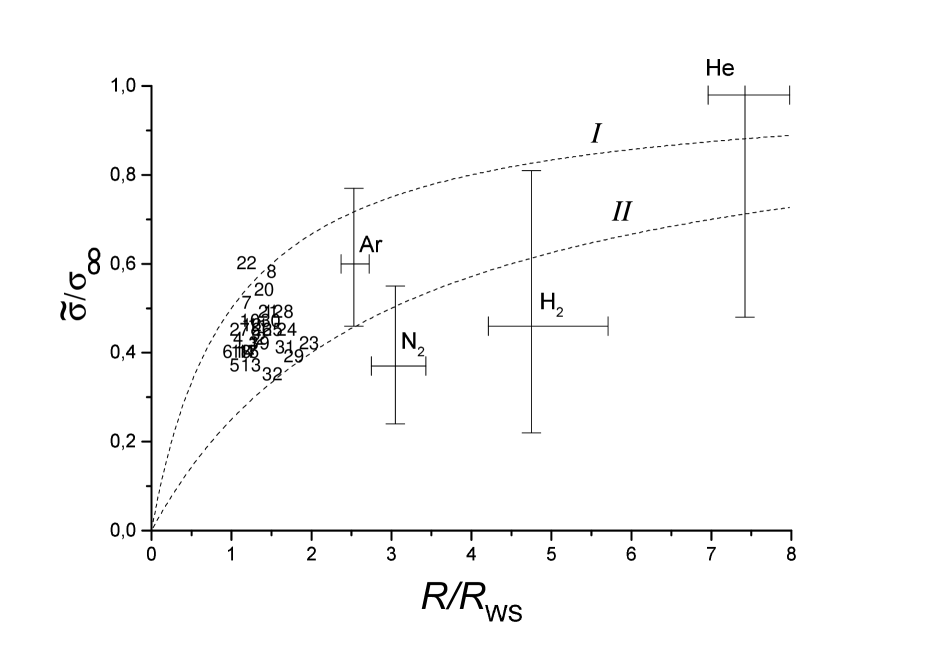
FIG. 5.:

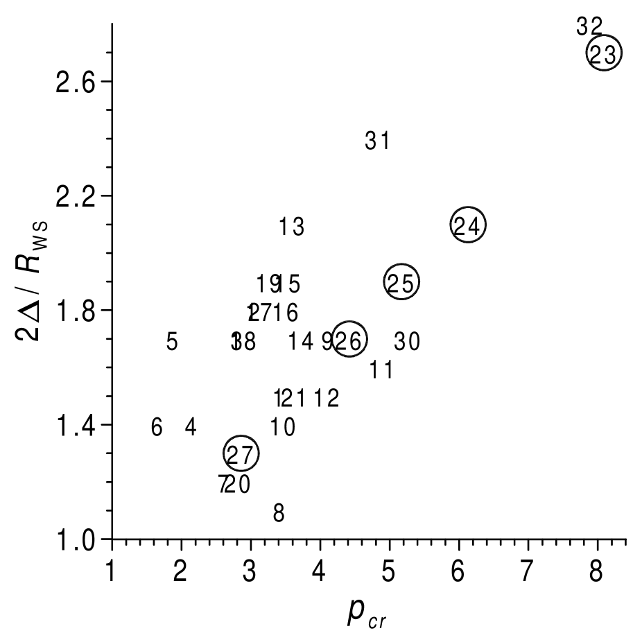
FIG. 6.:

TABLE I.: Some parameters of liquids and Ps bubbles, obtained within the infinite potential well model.

liquid		$R_{\rm WS}$	$\sigma_{\infty}$	$\tau_{\rm o-Ps}$	$\Theta_{\rm FWHM}$	$R_{\infty}$	$\delta$	$R$	${\displaystyle\frac{\tilde{\sigma}}{\sigma_{\infty}}}$	${\displaystyle\frac{2\Delta}{R_{\rm WS}}}$
		Å	${\displaystyle\rm\frac{dyn}{cm^{2}}}$	ns	mrad	Å	Å	Å
n-C5H12	n-pentane	3.583	15.32	4.25	2.25	7.4	2.0	5.4	0.43	2.0
n-C6H14	n-hexane	3.737	17.74	3.92	2.26	7.4	2.1	5.3	0.38	2.3
n-C7H16	n-heptane	3.881	19.65	3.85	2.33	7.1	2.0	5.1	0.37	2.2
n-C10H22	n-decane	4.267	23.3	3.49	2.47	6.7	2.0	4.7	0.38	1.8
n-C12H26	n-dodecane	4.492	24.84	3.43	2.43	6.8	2.0	4.8	0.33	2.2
n-C14H30	n-tetradecane	4.696	26.0	3.35	2.52	6.6	2.0	4.6	0.35	1.9
i-C8H18	isooctane	4.038	18.33	4.05	2.42	6.9	1.9	5.0	0.45	1.5
C(CH3)4	neopentane	3.656	11.52	5.15	2.21	7.5	1.9	5.6	0.53	1.4
C6H12	cyclohexane	3.509	24.65	3.24	2.45	6.8	2.1	4.7	0.38	2.2
C7H14	methylcyclohexane	3.692	23.28	3.50	2.49	6.7	2.0	4.7	0.41	1.8
C6H6	benzene	3.285	28.22	3.15	2.55	6.5	2.0	4.5	0.39	2.1
C6H5CH3	toluene	3.486	27.92	3.24	2.57	6.5	2.0	4.5	0.40	2.0
C2H5C6H5	ethylbenzene	3.654	28.74	3.02	2.44	6.8	2.1	4.7	0.32	2.8
(CH3)2C6H4	o-xylene	3.769	29.76	3.08	2.54	6.5	2.0	4.5	0.35	2.3
(CH3)2C6H4	m-xylene	3.658	28.47	3.20	2.49	6.7	2.0	4.7	0.34	2.4
(CH3)2C6H4	p-xylene	3.663	28.01	3.21	2.49	6.7	2.0	4.7	0.35	2.4
(CH3)3C6H3	mesitylene	3.748	27.55	3.21	2.49	6.7	2.0	4.7	0.35	2.3
(CH3)4C6H2	1,2,3,4-thetra-	3.888	29.	3.02	2.52	6.6	2.0	4.6	0.34	2.2
	methylbenzene
C6F6	hexafluorobenzene	3.572	22.63	3.78	2.39	7.0	2.0	5.0	0.37	2.4
Si(CH3)4	tetramethylsilane	3.780	13.20	4.75	2.25	7.4	1.9	5.5	0.49	1.5
(C2H${}_{5})_{2}$O	diethylether	3.453	16.65	3.82	2.29	7.6	2.1	5.2	0.44	1.9
1,4-C4H8O2	dioxane	3.234	32.61	3.02	2.86	5.8	1.8	4.0	0.52	1.1
CH3OH	methanol	2.528	22.12	3.58	2.29	7.2	2.1	5.2	0.37	3.5
C2H5OH	ethanol	2.855	21.97	3.50	2.35	7.1	2.1	5.0	0.39	2.7
C3H7OH	propanol	3.101	23.32	3.38	2.40	6.9	2.0	4.9	0.39	2.5
C4H9OH	butanol	3.311	24.93	3.36	2.46	6.7	2.0	4.7	0.39	2.3
C8H17OH	octanol	3.938	27.10	3.13	2.57	6.5	2.0	4.5	0.39	1.8
H2O	water	1.928	72.14	1.85	3.05	5.4	2.0	3.4	0.39	2.8
D2O	heavy water	1.930	70.89	1.95	2.87	5.8	2.1	3.7	0.31	4.1
(CH${}_{3})_{2}$CO	acetone	3.078	24.02	3.29	2.45	6.8	2.0	4.8	0.41	2.2
CH3CN	acetonitrile	2.756	28.66	3.30	2.44	6.8	2.0	4.8	0.35	3.2
CS2	carbon disulfide	2.880	31.58	2.20	2.35	7.1	2.5	4.6	0.29	3.9
He, 4.2 K	helium	2.350	0.096	99.1	0.86(6)	19.3	1.9	17.4	0.97${}^{+0.6}_{-0.5}$	0.2${}^{+9}_{-2}$
H2, 20.3 K	hydrogen	2.243	1.92	28.6	1.3(2)	12.8	2.1	10.7	0.44${}^{+0.34}_{-0.22}$	6.1${}^{+14}_{-5}$
N2, 77.3 K	nitrogen	2.395	8.85	11.0	1.8(2)	9.2	1.8	7.4	0.35${}^{+0.17}_{-0.13}$	5.7${}^{+6}_{-4}$
Ar, 86.4 K	argon	2.245	12.42	6.50	2.20(15)	7.6	1.8	5.8	0.56${}^{+0.15}_{-0.13}$	2.0${}^{+2}_{-1}$

$R_{\rm WS}$ is the radius of the Wigner-Seitz cell (calculated from the density and molecular mass).

$\sigma_{\infty}$ is the surface tension coefficient of a liquid with plane interphase boundary at room temperature (except the cases of liquified gases).

$\tau_{\rm o-Ps}$ is the o-Ps lifetime [12, 21].

$\Theta_{\rm FWHM}$ is the full width at half maximum of the narrow component of the ACAR spectra [12, 21].

$R_{\infty}=R+\delta$ is the radius of the Ps bubble, calculated from Eq.(3.21) using $\Theta_{\rm FWHM}$ values.

$\delta$ is the penetration depth of the outer electrons into the Ps bubble. It is obtained from Eq.(3.9) using $R_{\infty}$ and $\tau_{\rm o-Ps}$ values. $\tau^{0}_{\rm o-Ps}$ was adopted to be 0.5 ns in all cases except He (1.9 ns), H₂ (0.92 ns) and N₂ (0.56 ns).

Relative uncertainties of $\tau_{\rm o-Ps}$ and $\Theta_{\rm FWHM}$ are no more than 5 and 10% respectively (for liquified gases indicated in parenthesis). Uncertainty of $\tilde{\sigma}/\sigma_{\infty}$ is approximately four times larger than uncertainties of $\Theta_{\rm FWHM}$ (about 40%).

$2\Delta/R_{\rm WS}$ are calculated from Eq.(1.1) using respective values of $\tilde{\sigma}/\sigma_{\infty}$ and assuming $r\equiv R$ (in accord with Eq.(4.9)).

TABLE II.: Parameters of the Ps trap and microscopic surface tension obtained within the finite potential well model.

	liquid	$R_{U}$	$\delta$	$R$	$U$	$E$	$k_{U}R_{U}$	${\displaystyle\frac{\tilde{\sigma}}{\sigma_{\infty}}}$	$\tilde{\sigma}(R_{\sigma})$	${\displaystyle\frac{2\Delta}{R_{\rm WS}}}$	$p_{cr}$
		Å	Å	Å	eV	eV			${\displaystyle\rm\frac{dyn}{cm^{2}}}$		MPa
1	n-pentane	6.4	1.2	5.2	3.48	0.37	2.81	0.49	7.45	1.5	3.36
2	n-hexane	6.3	1.2	5.1	3.32	0.38	2.80	0.43	7.56	1.8	3.01
3	n-heptane	6.1	1.2	5.0	3.49	0.40	2.80	0.42	8.31	1.8	2.76
4	n-decane	5.7	1.1	4.6	3.66	0.45	2.78	0.43	9.99	1.4	2.10
5	n-dodecane	5.8	1.2	4.6	3.52	0.44	2.78	0.37	9.24	1.8	1.83
6	n-tetradecane	5.6	1.1	4.5	3.72	0.47	2.78	0.40	10.3	1.4	1.61
7	isooctane	5.9	1.1	4.8	3.91	0.43	2.80	0.51	9.27	1.1	2.57
8	neopentane	6.6	1.1	5.5	3.84	0.35	2.83	0.58	6.71	1.1	3.37
9	cyclohexane	5.7	1.2	4.5	3.43	0.45	2.77	0.44	10.8	1.7	4.07
10	methylcyclohexane	5.7	1.1	4.6	3.74	0.46	2.78	0.47	11.0	1.4	3.47
11	benzene	5.5	1.1	4.4	3.64	0.48	2.77	0.46	12.9	1.6	4.90
12	toluene	5.5	1.1	4.4	3.77	0.49	2.77	0.46	12.8	1.5	4.10
13	ethylebenzene	5.7	1.2	4.5	3.25	0.45	2.76	0.37	10.6	2.1	3.60
14	o-xylene	5.5	1.2	4.3	3.57	0.48	2.77	0.40	12.0	1.7	3.73
15	m-xylene	5.6	1.2	4.4	3.52	0.46	2.77	0.40	11.3	1.8	3.54
16	p-xylene	5.6	1.1	4.5	3.52	0.46	2.77	0.40	11.2	1.8	3.51
17	mesitylene	5.6	1.1	4.5	3.52	0.46	2.77	0.40	11.1	1.8	3.13
18	1,2,3,4-thetra-	5.5	1.2	4.3	3.46	0.48	2.76	0.40	11.6	1.7	2.9
	methylbenzene
19	hexafluorobenzene	5.9	1.1	4.8	3.64	0.42	2.79	0.42	9.47	1.9	3.27
20	tetramethylsilane	6.4	1.1	5.3	3.77	0.37	2.82	0.54	7.15	1.2	2.82
21	diethylether	6.2	1.2	5.0	3.36	0.39	2.80	0.49	8.23	1.5	3.64
22	dioxane	4.9	1.0	3.9	4.46	0.61	2.76	0.60	19.7	0.8	4.07
23	methanol	6.2	1.2	5.0	3.21	0.39	2.79	0.42	9.37	2.7	8.09
24	ethanol	6.0	1.2	4.8	3.33	0.41	2.78	0.45	9.91	2.1	6.13
25	propanol	5.9	1.2	4.7	3.39	0.43	2.78	0.45	10.4	1.9	5.17
26	butanol	5.7	1.1	4.6	3.54	0.45	2.78	0.45	11.1	1.7	4.42
27	octanol	5.4	1.1	4.3	3.69	0.49	2.77	0.45	12.2	1.3	2.86
28	water	4.3	1.1	3.2	3.64	0.73	2.68	0.49	35.6	1.7	22.1
29	heavy water	4.6	1.2	3.4	3.33	0.64	2.69	0.39	27.9	2.8
30	acetone	5.8	1.2	4.6	3.46	0.45	2.77	0.47	11.3	1.7	5.27
31	acetonitrile	5.8	1.2	4.6	3.44	0.44	2.77	0.41	11.7	2.4	4.85
32	carbon disulfide	5.7	1.4	4.3	2.43	0.43	2.71	0.35	11.2	2.8	7.90
	He, 4.2 K	18.6	1.1	17.5	3.74	0.05	3.02	0.98${}^{+0.6}_{-0.5}$	0.094	0.1${}^{+8}_{-2}$	0.23
	H2, 20.3 K	11.9	1.2	10.7	3.16	0.12	2.95	0.46${}^{+0.35}_{-0.23}$	0.88	5.7${}^{+13}_{-4}$	1.29
	N2, 77.3 K	8.4	1.1	7.3	4.05	0.23	2.90	0.37${}^{+0.18}_{-0.13}$	3.3	5.2${}^{+6}_{-3}$	3.39
	Ar, 86.4 K	6.7	1.0	5.7	4.50	0.35	2.86	0.60${}^{+0.17}_{-0.14}$	7.5	1.7${}^{+1.4}_{-1}$	4.90

Calculating parameters of the Ps bubble we adopted that $\pi r_{0}^{2}cZ_{\rm eff}n$ is approximately equal to 0.5 ns in all cases except He (1.9 ns), H₂ (0.92 ns) and N₂ (0.56 ns).

$2\Delta/R_{\rm WS}$ are calculated from Eq.(1.1) using respective values of $\tilde{\sigma}/\sigma_{\infty}$ and assuming $r\equiv R$ (in accord with Eq.(4.9)).

REFERENCES

- [1] R. C. Tolman, J. Chem. Phys. 17(3), 333 (1949)
- [2] Hirschfelder, J.O., Curtiss, Ch.F. and Bird, R.B. Molecular Theory of Gases and Fluids, John Wiley and sons. NY (1954)
- [3] J. Schmelzer, R. Mahnke, J. Chem. Soc., Faraday Trans. 1, 82, 1413 (1986)
- [4] A. I. Rusanov, Equilibrium of Phases and Surface Phenomena. (Khimiya, Leningrad, 1967).
- [5] V. M. Byakov, V. R. Petukhov, Radiochem. Radioanal. Lett. 58(2) 91 (1983).
- [6] H. Nakanishi, S. J. Wang, Y. C. Jean, In Positron Annihilation Studies of Fluids, ed. by S.C.Sharma (World Scientific, Singapore, 1988), p. 292.
- [7] V. M. Byakov, V. I. Grafutin, V. L. Grishkin et al., Chemical Physics (Khimicheskaya Fizika) 18(3), 75 (1999)
- [8] V. M. Byakov, S. V. Stepanov, Radiat. Phys. Chem. (2000), accepted for publication.
- [9] O. E. Mogensen, Positron Annihilation in Chemistry. Springer Series in Chemical Physics 58, (Springer-Verlag, Berlin 1995).
- [10] A. I. Akhiezer, V. B. Berestetskii, Quantum Electrodynamics, (Nauka, Moscow, 1981).
- [11] R. A. Ferrel, Phys. Rev. 108, 167 (1957).
- [12] H. Nakanishi, Y. C. Jean in Positron and Positronium Chemistry, ed. by D. M. Schrader and Y. C. Jean (Elsevier, Amsterdam 1988), Chapt.5. p.159.
- [13] A. T. Stewart, C. V. Briscoe, Positron Annihilation, Proceedings of the Conference. Wayne State University, ed. by A. T. Stewart and L. O. Roellig, (Academic Press, New York 1959), p. 383.
- [14] L. O. Roellig, Proc. Wayne State University Conf. on Positron Annihilation, ed. by A. T. Stewart and L. O. Roellig (Academic Press, New York 1967), p. 127.
- [15] T. Mukherjee, B. Ganguly, B. Dutta-Roy, J.Chem. Phys. 107(18), 7467 (1997).
- [16] T. Mukherjee, S. K. Das, B. Ganguly, B. Dutta-Roy, Phys. Rev. B 57(21), 13363 (1998).
- [17] D. Gangopadhyay, B. Ganguly, T. Mukherjee, B. Dutta-Roy, J. Phys.: Condens. Matter 11, 1463 (1999).
- [18] T. Mukherjee, D. Gangopadhyay, S. K. Das, B. Ganguly, B. Dutta-Roy J. Chem. Phys., 110(14), 6844 (1999).
- [19] S. Y. Chuang, S. J. Tao, Can. J. Phys. 51, 820 (1973).
- [20] K. Hirata, Y. Kobayashi, Y. Ujihira, J.Chem.Soc., Faraday Trans. 92 985 (1996).
- [21] A. T. Stewart, C. V. Briscoe, J. J. Steinbacher, Can. J. Phys. 68, 1362 (1990).
- [22] A. M. Askhabov, M. A. Ryazanov, Bull. Acad. Sci. USSR 362(5) 630 (1998).
- [23] M. I. Shakhparonov, B. G. Kalitkin, V. V. Levin, Zhurnal Fizicheskoj Khimii (in Russian) 46 498 (1972).
- [24] E. I. Akhumov, Zhurnal Fizicheskoj Khimii (in Russian) 60(12) 3038 (1972).