Abstract

We describe a numerical model for the interaction of light with large raindrops using realistic nonspherical drop shapes. We apply geometrical optics and a Monte Carlo technique to perform ray traces through the drops. We solve the problem of diffraction independently by approximating the drops with areaequivalent ellipsoids. Scattering patterns are obtained for different polarizations of the incident light. They exhibit varying degrees of asymmetry and depolarization that can be linked to the distortion and thus the size of the drops. The model is extended to give a simplified long-path integration.

1. Introduction

Large raindrops are deformed from spheres because of aerodynamic pressure as they fall at terminal velocity.${}^{\hbox{\immediate{\bf{?}},\penalty 1000\hskip 0.91003pt plus 0.70004pt minus 0.70004pt{\bf{?}},\penalty 1000\hskip 0.91003pt plus 0.70004pt minus 0.70004pt{\bf{?}}}}$ Beard and Chuang’s${}^{\hbox{\immediate{\bf{?}}}}$ (and Chuang and Beard’s${}^{\hbox{\immediate{\bf{?}}}}$) model results for the flattening at the base of the drops are used in this study. Drop shapes are specified by

$$r(\theta)=a[1+\sum_{n=0}^{10}c_{n}\cos(n\theta)]$$ (1)

where $a$ is the radius of the undistorted sphere, located at the center of mass of the drop; $\theta$ is the polar elevation with $\theta=0$^∘ pointing vertically downward (Fig. 1) and $c_{n}$ are shape co-efficients given in Table 1. Most previous research is restricted to spherical drops${}^{\hbox{\immediate{\bf{?}},\penalty 1000\hskip 0.91003pt plus 0.70004pt minus 0.70004pt{\bf{?}},\penalty 1000\hskip 0.91003pt plus 0.70004pt minus 0.70004pt{\bf{?}}}}$ or ellipsoid particles.${}^{\hbox{\immediate{\bf{?}}}}$ Macke and Gro klaus${}^{\hbox{\immediate{\bf{?}}}}$ used the same distorted drop shapes as the present study for backscattering applicable to lidar measurements of rainfall intensities. In the current study we are interested in using drop distortion in a forward-scatter mode so as to measure drop size and, for long paths, rainfall intensity. A complete description of the model, including its application to a long path integration, can be found in Ross.${}^{\hbox{\immediate{\bf{?}}}}$

2. The Ray Trace Method

We used a Monte Carlo approach in which a large number of photons are traced through the drop using geometrical optics. Diffraction is accounted for analytically. For our simulation we chose a wavelength of $\lambda=650\,\mathrm{nm}$, and thus the size parameter $x=2\pi a/\lambda$ is in the range $5\cdot 10^{3}\lesssim x\lesssim 4\cdot 10^{4}$ for the drop sizes in Table 1. Glantschnig and Chen${}^{\hbox{\immediate{?}}}$ found that geometrical optics produced good results in comparison with the rigorous Mie theory for $x\geq 20$ and scattering angles $\leq 60^{\circ}$. Macke et al. ${}^{\hbox{\immediate{\bf{?}}}}$ found this condition to be $x\geq 60$. In a different study,${}^{\hbox{\immediate{\bf{?}}}}$ computations were carried out over a wide range of size parameters. The results showed that the deviation from Mie theory is less than 1% for size parameters $x\approx 10^{4}$ and $m=1.33$, confirming the validity of our geometrical optics approach.

A. Forward Scattering

Table 2, adapted from van de Hulst,${}^{\hbox{\immediate{\bf{?}}}}$ gives the forward- and backward-scattered intensities for spherical scatterers and polarizations perpendicular and parallel to the scattering plane (polarization 1 and 2, respectively). Over 91% of light of polarization 1 and more than 97% of polarization 2 is forward scattered. As can be seen from Table 2, upward of 99.5% of the total forward-scattered light for both polarizations emerges from the first interface after simple reflection ($p=0$) and from the second interface after twofold refraction ($p=1$). The fraction of forward-scattered intensity in the $p=0$ and $p=1$ rays increases for more distorted drops (see Section 4), and so it is sufficient to consider only the contributions of these rays to forward scattering.

B. The Procedure

Fig. 2 shows the flow diagram for the ray trace model. The model is run with $N=10^{8}$ photons. Runs for different polarizations of the incident light use the same set of random photons to exclude statistical variations as a possible cause for differences in the

Table 1: Shape co-efficients for cosine distortion fit (Eq. (1)) for drop radii between 0.5 and 4.5$\,\mathrm{mm}$ from Chuang and Beard.${}^{\hbox{\immediate{?}}}$

a [1pt] [mm]	Shape co-efficients ($c_{n}\cdot 10^{4}$) for $n=$
	0	1	2	3	4	5	6	7	8	9	10

0.5	-28	-30	-83	-22	-3	2	1	0	0	0	0
0.75	-72	-70	-210	-57	-6	7	3	0	-1	0	1
1.0	-134	-118	-385	-100	-5	17	6	-1	-3	-1	1
1.25	-211	-180	-592	-147	4	32	10	-3	-5	-1	2
1.5	-297	-247	-816	-188	24	52	13	-8	-8	-1	4
1.75	-388	-309	-1042	-221	53	75	15	-15	-12	0	7
2.0	-481	-359	-1263	-244	91	99	15	-25	-16	2	10
2.25	-573	-401	-1474	-255	137	121	11	-36	-19	6	13
2.5	-665	-435	-1674	-258	187	141	4	-48	-21	11	17
2.75	-755	-465	-1863	-251	242	157	-7	-61	-21	17	21
3.0	-843	-472	-2040	-240	299	168	-21	-73	-20	25	24
3.25	-930	-487	-2207	-222	358	175	-37	-84	-16	34	27
3.5	-1014	-492	-2364	-199	419	178	-56	-93	-12	43	30
4.0	-1187	-482	-2650	-148	543	171	-100	-107	2	64	32
4.5	-1328	-403	-2889	-106	662	153	-146	-111	18	81	31

scattering patterns. The photons propagate parallel to the $x$ axis from negative $x$ toward

Table 2: Separation into forward and backward scattering for polarisations 1 (first number in each column) and 2.

Ray	Forward		Backward		Total
$p=0$	857	248	163	59	1020	307
$p=1$	8217	9456	0	0	8217	9456
combined	9074	9704	163	59	9237	9763
$p\geq 2$	44	15	719	222	763	237
All $p$	9118	9719	882	281	10,000	10,000

the drop, and a point $\mathbf{P}$ on the drop’s surface can be represented in Cartesian coordinates by

$$\mathbf{P}=r(\theta)\left[\begin{array}[]{c}-\sin{\phi}\sin{\theta}\\ \cos{\phi}\sin{\theta}\\ -\cos{\theta}\end{array}\right]$$ (2)

where $\phi$ is the azimuth angle, increasing clockwise from the $y$-axis. The surface normal at $\mathbf{P}$ is

$$\mathbf{N}=\left(\frac{\partial{\mathbf{P}}}{\partial\theta}\times\frac{\partial{\mathbf{P}}}{\partial\phi}\right)\,.$$ (3)

Using Snell’s law and the Fresnel equations, we can now trace the photons through the drop. The detector coordinates ($\Theta$,$\Phi$) are defined similarly to ($\theta$,$\phi$), and arriving photons are resolved into angular bins of 1^∘ resolution in $\Theta$ and $\Phi$.

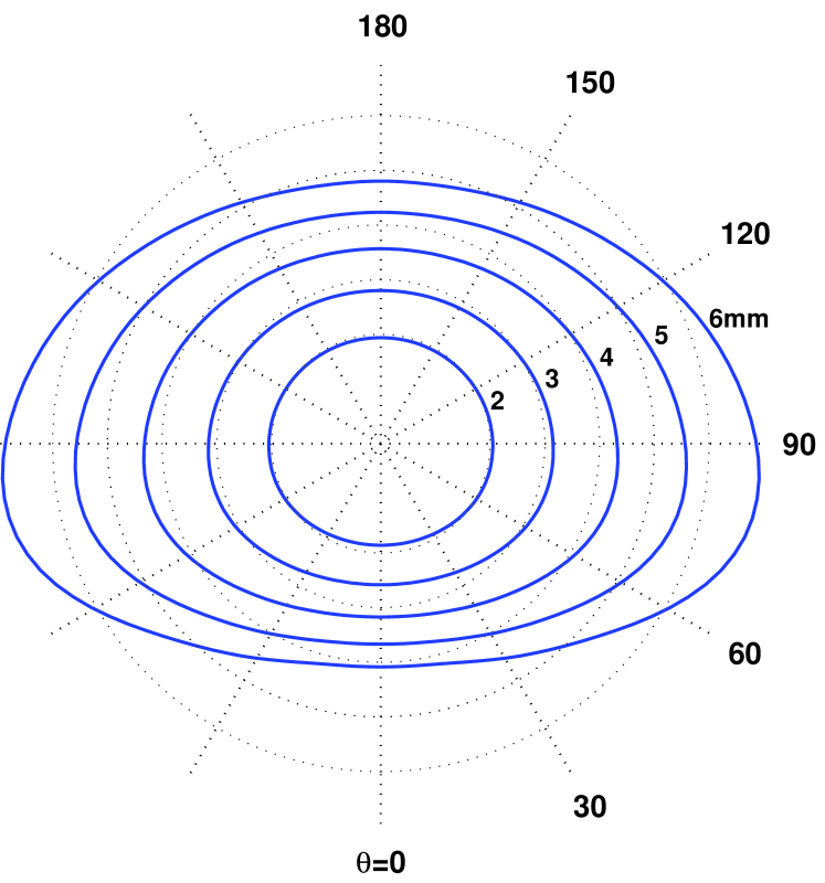
Fig. 1: Drop shapes for diameters $D=2$, 3, 4, 5 and 6$\,\mathrm{mm}$ with dashed circles shown for comparison and the angle $\theta$ in the coordinate system used.

Each photon generated is assigned a weight of one. The intensity fractions for $p=0$ and $p=1$ are stored in an intensity matrix $\mathbf{I}$ with $\Theta$ and $\Phi$ as row and column indices, respectively.

3. Diffraction

Analytic solutions for diffraction from distorted drop shapes do not exist. Here, drop shapes are approximated by area-equivalent ellipsoids, for which the diffraction pattern is known.

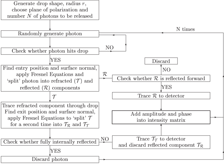
Fig. 2: Flowchart for the ray trace.

This approximation is verified when the exact diffraction problem is numerically solved for one of the larger drops. Results showed negligible differences at the angular resolution used.

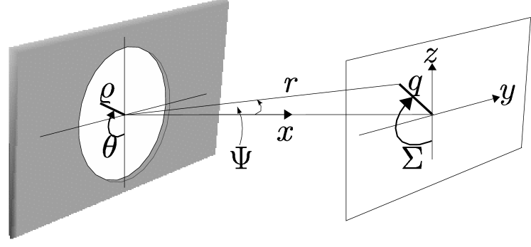
Fig. 3: Co-ordinate system used for the diffraction integral in Eq. (4).

Given the range of size parameters in this study, diffraction scatters energy equal to refraction and reflection combined,${}^{\hbox{\immediate{\bf{?}},\penalty 1000\hskip 0.91003pt plus 0.70004pt minus 0.70004pt{?}}}$ i.e., the extinction efficiency is 2.

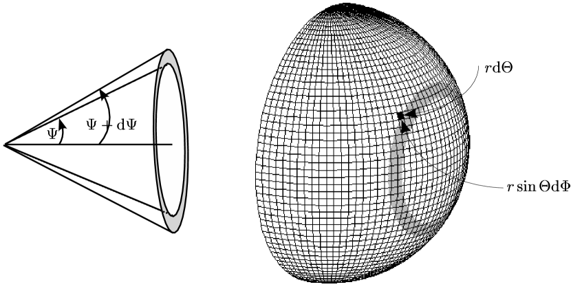
Fig. 4: The energy ring (left) and its projection onto the spherical detector.

A. Diffraction from Spheres

The framework for the elliptical approximation is based on diffraction from a spherical aperture:${}^{\hbox{\immediate{\bf{?}},\penalty 1000\hskip 0.91003pt plus 0.70004pt minus 0.70004pt{\bf{?}}}}$

$$\mathscr{E}(q,\Sigma) = \frac{{\mathcal{E}}_{A}\ \exp{[i(\omega t-kr)]}}{r}\ \int\limits_{\varrho=0}^{a}\int\limits_{\theta=0}^{2\pi}\ \exp{[i(k\varrho q/r)}$$ (4)

$$\times\cos(\theta-\Sigma)]\ \varrho\ d\varrho\ d\theta\,,$$

where $\mathscr{E}$ is the electric field amplitude, giving intensity $I\propto|\mathscr{E}|\/^{2}$. ${\mathcal{E}}_{A}$ denotes the source strength per unit area of the aperture; and $r$ the distance between its center and the detector (Fig. 3). The solution is

$$I\propto\left[\frac{\mathscr{J}_{1}(kaq/r)}{kaq/r}\right]^{2}=\left[\frac{\mathscr{J}_{1}(ka\sin\Psi)}{ka\sin\Psi}\right]^{2}\,,$$ (5)

where $a$ is the radius of the aperture, $k$ is the wave number 2$\pi/\lambda$, and $\mathscr{J}_{1}$ is the Bessel function of the first kind and order one. The solution does not depend on the angle $\Sigma$ due to the circular symmetry. By integrating relation 5, we write the fraction of the total intensity contained within a cone of angle $\Psi$ as

$$L(\Psi)=1-\mathscr{J}_{0}^{2}(ak\sin(\Psi))-\mathscr{J}_{1}^{2}(ak\sin(\Psi))\,,$$ (6)

where $\mathscr{J}_{0}$ is the Bessel function of order zero.${}^{\hbox{\immediate{\bf{?}}}}$

If the energy flux through a ring element of area $2\pi r^{2}\sin\Psi\;\mathrm{d}\Psi$ (Fig. 4) is $L^{\prime}(\Psi)\;\mathrm{d}\Psi$, then the fractional flux through a detector element of angular dimensions (d$\Theta$,d$\Phi$) and area $r^{2}\sin\Theta\;\mathrm{d}\Theta\;\mathrm{d}\Phi$ is

$$L^{\prime}(\Psi)\frac{\sin\Theta\;\mathrm{d}\Theta\;\mathrm{d}\Phi}{2\pi\sin\Psi}$$ (7)

which can be expressed in terms of detector coordinates because $\cos\Psi=\sin\Theta\sin\Phi$. After this substitution and further simplifications, the final result is

$$\tilde{I}_{\Theta\Phi}=\frac{1}{2\pi}\int\limits_{\Delta\Theta}\int\limits_{\Delta\Phi}\frac{2\mathscr{J}_{1}^{2}(ak\xi)\sin^{2}\Theta\sin\Phi}{\xi^{2}}\;\mathrm{d}\Theta\;\mathrm{d}\Phi$$ (8)

where $\xi$ stands for $\left[\cos^{2}{\Theta}+\cos^{2}{\Phi}\sin^{2}{\Theta}\right]^{1/2}$. The intervals $\Delta\Theta$ and $\Delta\Phi$ are appropriately chosen to cover the size of the bin. By analogy with the intensity matrix introduced in Subsection 2.B, this yields the $181\times 181$ intensity matrix $\tilde{\mathbf{I}}$ for diffraction, which we find numerically.

B. Approximating the Drop Shapes with Ellipsoids

The Fraunhofer diffraction integral for the distorted drops has no analytic solution as $\varrho$ is a function of $\theta$. Hence we approximate the drops with areaequivalent ellipsoids. The cross-sectional area of the drops can be calculated from

$$A = \frac{1}{2}\oint_{C}r^{2}(\theta)\;\mathrm{d}\theta=a^{2}\int\limits_{0}^{\pi}\left[1+\sum_{n=0}^{10}c_{n}\cos(n\theta)\right]^{2}\;\mathrm{d}\theta$$ (9)

$$= \pi a^{2}\left[1+2c_{0}+c_{0}^{2}+\sum_{n=1}^{10}\frac{c_{n}^{2}}{2}\right]$$

with the co-efficients $c_{n}$ from Table 1. The discrepancy between the approximation and the actual drop shapes is the largest for the bigger drops and vanishes as the size (and the flattening at the base) of the drop decreases. Fig. 5 shows some examples.

Extending the circular aperture in one direction by a constant factor $\mu$ will cause the diffraction pattern to contract in that direction by the same factor. Because of the $\mu$ times larger area of the aperture, the intensity is $\mu^{2}$ times the original intensity at each point mapped from the original pattern.${}^{\hbox{\immediate{\bf{?}},\penalty 1000\hskip 0.91003pt plus 0.70004pt minus 0.70004pt{?}}}$ Hence we can calculate the contribution to each bin from diffraction using elliptic obstacles from the results of a circular aperture.

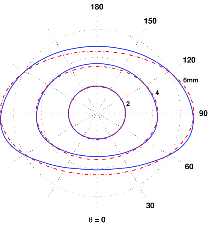
Fig. 5: Comparison between the ellipses used (dash-dot line) and the actual drop shapes for drop diameters $D=2$, 4 and 6$\,\mathrm{mm}$.

C. Verifying the Elliptic Approximation

In this subsection the diffraction integral is evaluated numerically for one exact drop shape. The results are used to validate the elliptic approximation. The constant radius $\varrho$ in Eq. (4) is replaced by the cosine distortion fit from Eq. (1), and the variable of integration is changed from $\varrho$ to $a$, the radius of the undistorted sphere. Eq. (4) becomes

$$\mathscr{E}(q,\Sigma)=\underbrace{\frac{\mathcal{E}_{A}\>\exp{[i(\omega t-kr)]}}{r}}_{C}\int\limits_{a=0}^{R}\int\limits_{\theta=0}^{2\pi}$$ (10)

$$\times \exp\left[i(kqa/r)\,\cos(\theta-\Sigma)\left(1+\sum_{n=0}^{10}c_{n}\,\cos(n\theta)\right)\right]$$

$$\times a\,\left(1+\sum_{n=0}^{10}c_{n}\,\cos(n\theta)\right)^{2}\;\mathrm{d}a\;\mathrm{d}\theta\,.$$

To simplify Eq. (10), the following substitutions can be applied

$$\chi=\frac{kq}{r}\cos(\theta-\Sigma),\xi=\left(1+\sum_{n=0}^{10}c_{n}\cos(n\theta)\right)$$ (11)

$$\Rightarrow\mathscr{E}(q,\Sigma)=C\int\limits_{a=0}^{R}\int\limits_{\theta=0}^{2\pi}\exp{(i\chi\xi a)}\>a\,\xi^{2}\;\mathrm{d}a\;\mathrm{d}\theta$$ (12)

$$= -\,C\int\limits_{\theta=0}^{2\pi}\left[\frac{\exp{(i\chi\xi\,a)}}{\chi^{2}\xi^{2}}\>(i\chi\xi\,a-1)\right]_{a=0}^{R}\,\xi^{2}\;\mathrm{d}\theta$$ (13)

$$= -\,C\int\limits_{\theta=0}^{2\pi}\frac{\exp{(i\chi\xi R)}\,(i\chi\xi R-1)+1}{\chi^{2}}\;\mathrm{d}\theta\,.$$ (14)

The integrand in Eq. (14) is resolved into its real and imaginary components

$$\mathscr{E}(q,\Sigma)= C \left[\;\int\limits_{\theta=0}^{2\pi}\frac{\chi\xi R\sin(\chi\xi R)+\cos(\chi\xi R)-1}{\chi^{2}}\;\mathrm{d}\theta\right.$$ (15)

$$+ \left.i\int\limits_{\theta=0}^{2\pi}\frac{\sin(\chi\xi R)-\chi\xi R\cos(\chi\xi R)}{\chi^{2}}\;\mathrm{d}\theta\right]$$

which can be evaluated numerically for a given pair of detector coordinates (q,$\Sigma$). To return to the original detector coordinates $(\Theta,\Phi)$ it can be shown that

$$\frac{q}{r}\cos(\theta-\Sigma)=\cos\theta\cos\Theta-\sin\theta\cos\Phi\,.$$ (16)

Making the replacements in Eq. (10) and (11) leads to the same integral as in Eq. (14) except that $\chi$ now represents $k$ times the right-hand side of Eq. (16) instead of the left-hand side.

Because $I\propto|\mathscr{E}|^{2}$, only the real part of Eq. (15) needs to be solved. Fig. 6 shows the results obtained for a distorted drop with radius $a=3\,\mathrm{mm}$. The

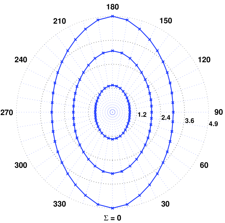
Fig. 6: Location of the first three minima in the diffraction pattern from a drop with radius $a=3$$\,\mathrm{mm}$.

locations of the first three minima exhibit a clear elliptic symmetry. The dotted lines emerging radially from the center represent the lines along which the integrations were carried out. The dotted circles with numbers next to them give the lines of constant $\Psi$ as percentages of a degree. The resolution for the integration was 10,000 points/deg, which gives approximately 500 points from the center of Fig. 6 to the outermost circle.

A continuous plot of the field amplitudes $\mathscr{E}(q,0^{\circ})$ and

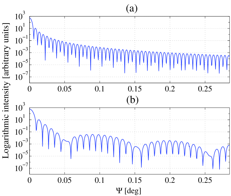
Fig. 7: Logarithmic intensity distribution for the directions (a) $\Sigma=90^{\circ}$ and (b) $\Sigma=0^{\circ}$.

$\mathscr{E}(q,90^{\circ})$ is shown in Fig. 7. The eccentricity of the pattern is obvious. The first minimum in the $\Sigma=90$^∘ direction is considerably closer to the center, indicating the contraction in the horizontal. A similar comparison between $\mathscr{E}(q,0^{\circ})$ and $\mathscr{E}(q,180^{\circ})$ (not shown) yields two identical curves within the margin of error, confirming the symmetry of the pattern about the horizontal. An interesting feature is the somewhat elongated sixth maximum in the $\Sigma=0^{\circ}$ direction. This feature returns in a similar shape with every 11th maximum.

A more quantitative account of the possible flattening in the pattern for the 3-mm drop can be obtained from $\aleph(q)=(\mathscr{E}(q,270^{\circ})-\mathscr{E}(q,90^{\circ}))/\mathscr{E}(q,90^{\circ})$, which gives a measure for the relative deviation from horizontal symmetry. Values do not exceed 0.4% and are only notably over 0.1% within 0.1^∘ of the central forward direction. We believe that this fully justifies the elliptic approximation, especially given the applied angular resolution of 1^∘ and also considering that the distortion decreases for smaller drops. The same computations can be carried out along the $\Sigma=0$ and $\Sigma=180$^∘ directions. Values in the absolute deviation do not exceed $4\cdot 10^{-6}$, which is the region of error applied during the numerical integration and can thus be neglected.

4. Results

The results from the computer model are presented separately for the ray trace (no diffraction) and for scattering including diffraction. The scattering patterns are displayed by a sinusoidal projection method (which means that the meridians appear as sine functions), hence the scale is preserved only on the central meridian and along the lines of latitude. This projection method also renders the region around the central forward direction without distortions.

A. Scattering from Single Drops – excluding Diffraction

The phase is omitted because the path lengths of the photons arriving at a particular bin can differ by several tens of wavelengths. These effects cancel out for a large number of photons and do not contribute any valuable information to the pattern.

Fig. 8 shows the scattering patterns for a 3-mm drop and $10^{8}$ photons. In Fig. 8(a) the incoming light was unpolarized. The pattern exhibits a symmetry about the central meridian that is to be expected from the rotational symmetry of the drops about their vertical axis. This can also be observed in the corresponding polar plot of

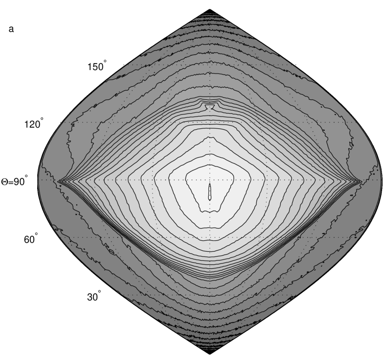
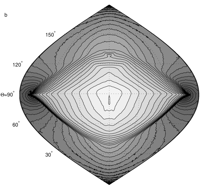
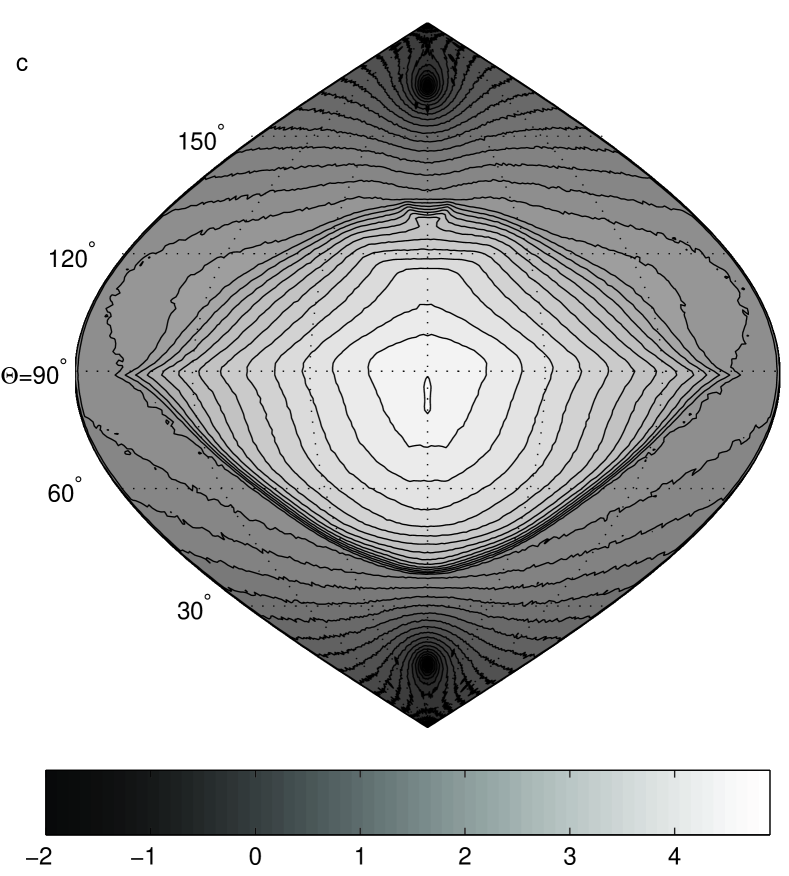
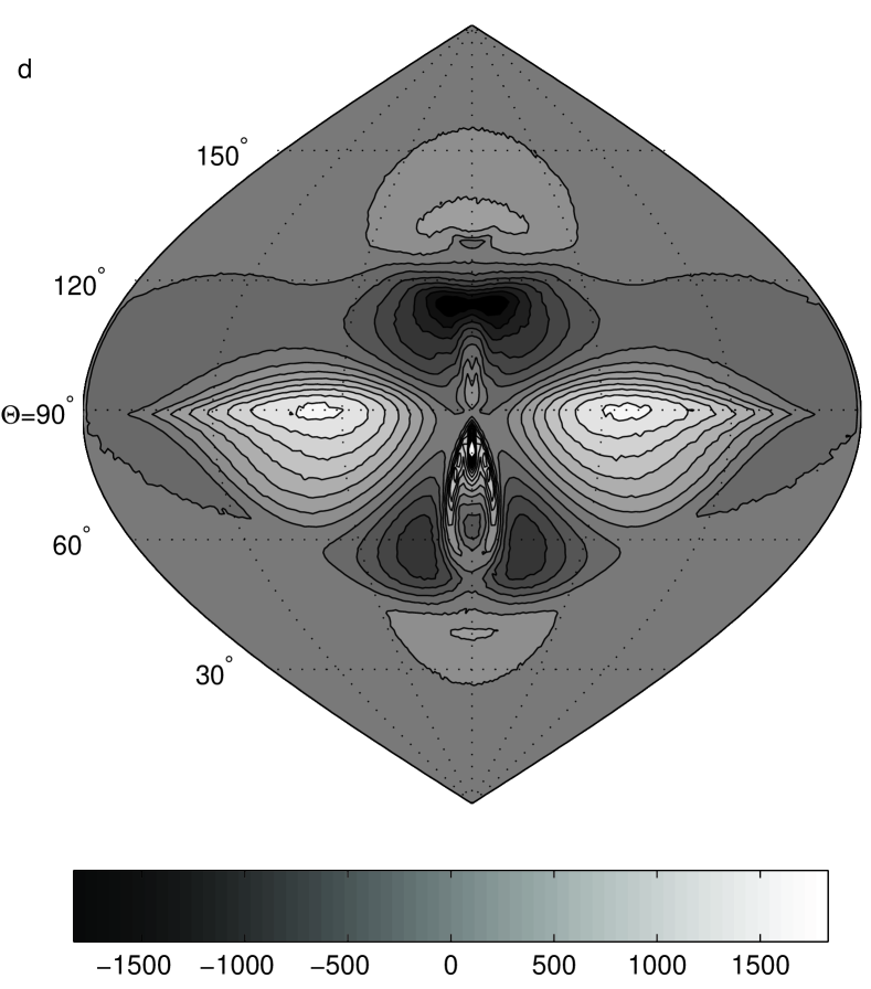
Fig. 8: Contour plots of the intensity distribution obtained from a 3$\,\mathrm{mm}$ drop, for: (a) unpolarised light, (b) $y$- and (c) $z$-polarised light. A plot of the difference in the obtained intensities for $y$-polarised and $z$-polarised light (non-logarithmic) is shown in (d). Note that the gray scale below (c) applies for (a) to (c) while (d) being the only non-logarithmic plot has a scale of its own.

Fig. 9(a) that shows the intensity distribution along the $\Theta=82^{\circ}$ line that contains the absolute maximum. The concentric semicircles are lines of constant intensity, and the numbers give the corresponding intensities as powers of ten. Fig. 9(b) shows the distribution along the $\Phi=90^{\circ}$ meridian. A distinguishing feature is the lack of symmetry about the equator. The absolute maximum has shifted from the equator ($\Theta=90^{\circ}$) to $\Theta=82^{\circ}$. It is accompanied by another local maximum at $\Theta=130^{\circ}$. For smaller drop sizes, the absolute maximum shifts closer to the (90^∘,90^∘) direction again.

Another prominent feature in Fig. 8(a) is the sharp gradient, creating a steep

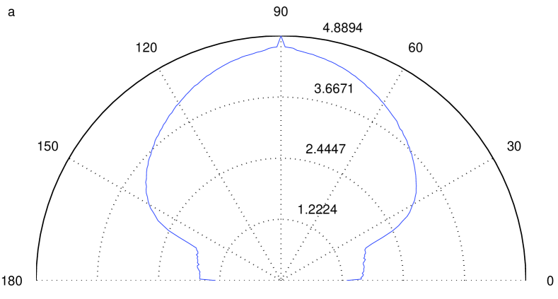
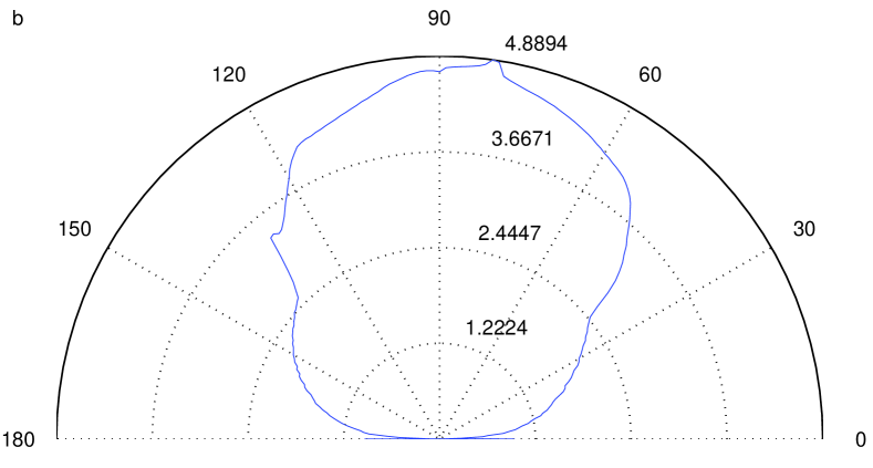
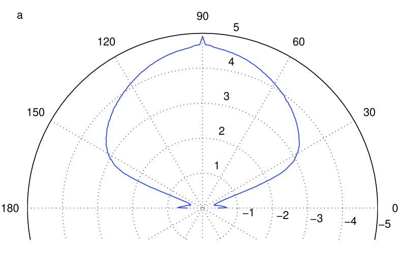
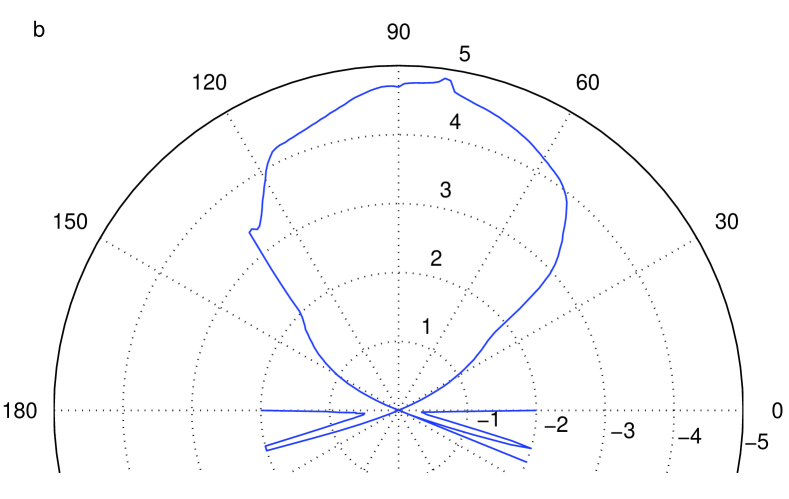
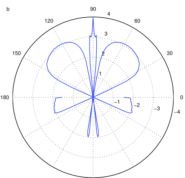
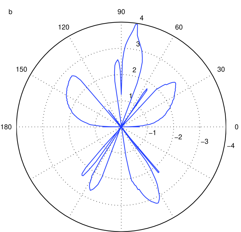
Fig. 9: Polar plots for a 3$\,\mathrm{mm}$ drop showing the intensity distribution along: (a) $\Theta=82^{\circ}$ and (b) $\Phi=90^{\circ}$, both for unpolarised light; (c) $\Theta=82^{\circ}$ for $y$-polarised light and (d) $\Phi=90^{\circ}$ for $z$-polarised light. The graphs in (e) and (f) show the difference between the results for $y$- and $z$-polarised light along $\Theta=81^{\circ}$ and $\Phi=90^{\circ}$ respectively. Negative values are plotted into the lower half of the circles.

intensocline that separates the central area of relatively high intensity from the outer, low-intensity regions. It is identified by the narrowly spaced contour lines. The model was used to record the intensities from the rays $p=0$ and $p=1$ separately. The light that arrives outside the intensocline has mostly undergone a single reflection at the first interface, whereas the high-intensity area is mainly lit by the twice-refracted rays.

Fig. 8(b) shows the pattern for the same drop but with incident light polarized parallel to the $y$ axis. There are two distinct minima near the equator at extreme angles for $\Phi$. This can also be seen on the corresponding polar plot Fig. 9(c). The sum of contributions from all angular bins is slightly ($\approx 1\%$) larger than for unpolarized light. The opposite is true if the incident light is polarized parallel to the $z$ axis as shown in Fig. 8(c): The distinct minima are on the $\Phi=90^{\circ}$ meridian, symmetrically at $\Theta=90^{\circ}\pm 74^{\circ}$. Light that is reflected into the angular bins containing the observed minima in Figs. 9(c) and 9(d) originates from points on the drop’s surface where the angle of incidence is at the Brewster angle of $\alpha_{p}=53.06^{\circ}$ and where the plane of polarization of the incident light is parallel to the scattering plane.

Fig. 8(d) shows the difference between the results obtained for $y$-polarized and $z$-polarized incident light. This plot shows the absolute deviation, and the minima that can be seen in Figs. 8(b) and 8(c) do not appear. There is, however, a significant difference in the high-intensity area, inside the intensocline and especially near the absolute maximum. Note that the scale of this last plot is nonlogarithmic to allow for both positive and negative differences. A high-intensity ridge that extends from $\Theta=78^{\circ}$ to $\Theta=86^{\circ}$ on the central meridian contains values that exceed the maximum value covered by the scale (compare with Fig. 9(f)). The actual maximum in Fig. 8(d) is 9200 and is located at $\Theta=81^{\circ}$. The maximum difference of 9200 photons at the central maximum is equivalent to 12.5% in relative terms, which explains why this feature does not appear on the individual contour plots in Figs. 8(b) and 8(c). If the pattern in Fig. 8(d) is divided by the (nonlogarithmic) intensity from Fig. 8(a) (result not shown), the extrema outside the intensocline visible in Figs. 8(b) and 8(c) can be observed. The intensity difference at these extrema is nearly twice the intensity value that is obtained there for unpolarized incident light. If the incident light is unpolarized, the reflectance $R$ at $\alpha_{p}$ is half of the value of $R_{\bot}$. Because $R_{\|}$ is equal to zero, the difference between the $y$- and $z$-polarized intensity is equal to $R_{\bot}$. Dividing $R_{\bot}$ by $R$ for unpolarized light thus always yields 2. The finite size of the angular bins allows inclusion of rays for which the angle of incidence differs slightly from $\alpha_{p}$. This should always keep the absolute value of the extremes slightly below 2. A drop of radius $a=0.5\,\mathrm{mm}$, for example, has its extreme values

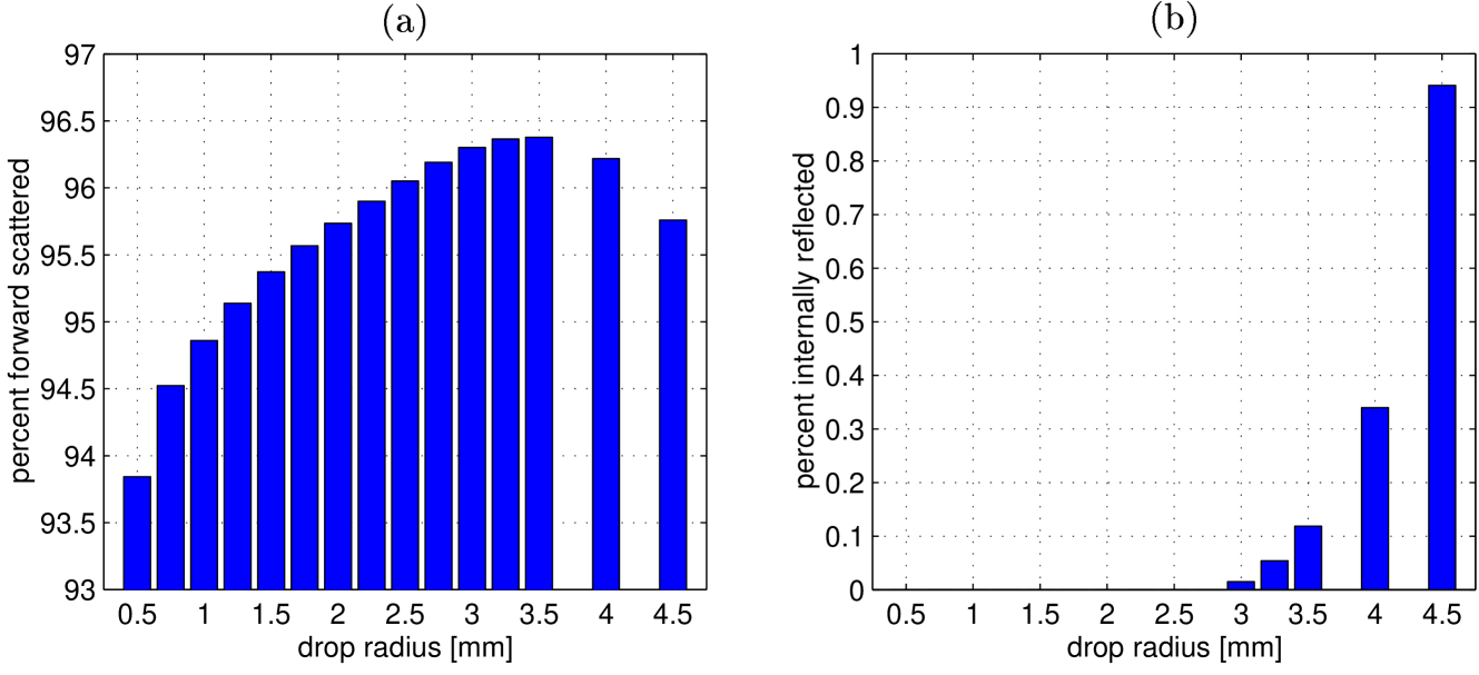
Fig. 10: (a) The fraction of the total incident intensity that is forward scattered and (b) the fraction of all incident rays that are entirely internally reflected (regardless of their intensity).

at 1.98 and -1.95, and the corresponding values for spherical drops are $\pm 1.95$. The reason why this is not observed for larger drops along the central meridian might be a combination of the varying curvature along the vertical axis and statistical fluctuations because the bins at such extreme angles contain only approximately 35 photons out of the total of 100 million.

Fig. 9(e) gives a clearer image of what happens along the $\Theta=81^{\circ}$ latitude. The scale is again logarithmic to accommodate the large spread of values. The pattern is dominated by the central maximum and two broad maxima on each side. For smaller drop sizes the central maximum becomes less dominant and is almost nonexistent for a 1-mm drop. The two peripheral maxima, however, remain almost constant in size and location.

Fig. 9(f) shows the intensity distribution along the central meridian. It is characterized by closely spaced maxima and minima. There is a general decrease in the number of significant extrema to be observed with decreasing drop size, accompanied by a general increase in overall symmetry.

Over 99.5% of the forward-scattered light from spherical scatterers emerges from either single reflection (ray $p=0$) or twofold refraction ($p=1$). The assumption was made that this would be similar for distorted drops, thus justifying rays with $p>1$ being neglected.

Fig. 10(a) shows the percentages of forward-scat-tered intensity in $p=0$ and $p=1$ for unpolarized incident light and drop sizes ranging from $a=0.5\,\mathrm{mm}$ to $a=4.5\,\mathrm{mm}$. The fraction of forward-scattered intensity increases with drop size, reaching a maximum for drops with $a=3.5\,\mathrm{mm}$. The rapid decline for larger drops can be explained from Fig. 10(b), which shows the percentage of photons that are internally reflected and thus discarded by the model. It can be seen that internal reflection can be neglected for most drop sizes and becomes noticeable only for large drops.

To be able to give a quantitative comparison with some tabulated values, the model was used to find the scattering pattern that would be produced by unpolarized light that is incident on a sphere of radius 0.1$\,\mathrm{mm}$. The result is given in Table 3. It compares

Table 3: Comparing results from the Computer Model and van de Hulst .${}^{\hbox{\immediate{?}}}$

Source:	model	van de Hulst
% forward scattered in p=0 and p=1
	93.73	93.89

the fraction of energy that is scattered forward in rays $p=0$ and $p=1$ from the computer model and Table 2.

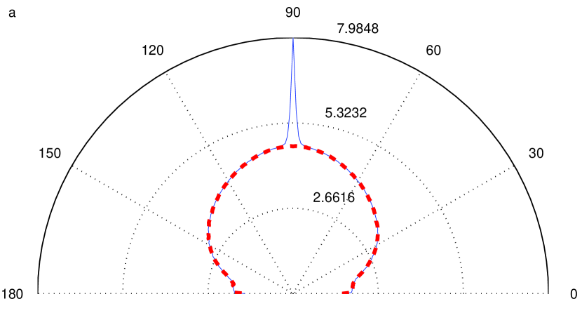
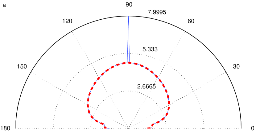
Fig. 11: Superposition of the polar plots of the logarithmic intensity including all components (continuous line) and without diffraction (dashed line) along the 90^∘ latitude for (a) $a=0.1\,\mathrm{mm}$ and (b) $a=3\,\mathrm{mm}$.

These differ by less than 0.2%, justifying the model and its assumptions.

B. Scattering from Single Drops – including Diffraction

The diffraction pattern is dominated by a narrow diffraction peak in the central forward direction. The width of this diffraction peak depends on the size of the scatterer. The effects of diffraction are therefore demonstrated for two extreme drop sizes: a 0.1-mm spherical drop and a 3-mm drop. Figures 11(a) and 11(b) show the combination of diffraction and ray trace together with the results from the ray trace alone. The central maximum for the 3-mm drop is much sharper and slightly higher than for the smaller drop. The solid and dashed curves only differ noticeably near the central diffraction peak, whereas the intensity at other angles is almost unchanged. This is significant for the design of an instrument to measure drop sizes. If the detectors are placed well off the central diffraction peak, the results can be simulated with contributions from the ray trace only. This is illustrated in a more quantitative form in Fig. 12. It shows the percentile change of the intensity distribution from the ray trace after diffraction is added. For the large 3-mm drop, the pattern is affected only by diffraction for angles of $\Psi\lesssim 1^{\circ}$ if we accept a 1% margin of error. For the smaller drop the same criterion would yield the condition $\Psi\lesssim 10^{\circ}$.

5. Practical Application

If a large number of individual field measurements is averaged, the underlying pattern linking the rainfall rate with drop diameter shows an exponential character as first proposed by Marshall and Palmer.${}^{\hbox{\immediate{\bf{?}}}}$ They suggested the following empirical relationship, the so-called Marshall Palmer distribution:

$$N(D)=N_{0}\exp{(-\Lambda D)},\qquad N_{0}=0.08\,{\rm cm}^{-4};$$ (17)

where $N(D){\rm d}D$ is the number of drops per unit volume having diameters between $D$ and $D+{\rm d}D$. The intercept parameter $N_{0}$ gives the intercept with the ordinate for $D=0$. The distribution depends entirely on the parameter $\Lambda$ that is determined by the rainfall rate $R$: $\Lambda=41R^{-0.21}$ where $R$ is in millimeters per hour and $\Lambda$ is in inverse centimeters.

We can now establish a function $P(D)$ to represent the cumulative probability of finding a drop with a diameter between 0 and D in a large enough sample:

$$P(D)=1-\exp{(-\Lambda D)}$$ (18)

If the drops are approximated as spheres of area $\pi/4\,D^{2}$ (which is possible because the number of drops decreases rapidly as the distortion increases - see Eq. (18)) and by integrating Eq. (17) (while neglecting the constants $N_{0}$ and $\pi/4$ that both cancel out in the normalization), one obtains the following area distribution:

$$\int\limits_{0}^{D}{D^{\prime}}^{2}\;\exp{(-\Lambda D^{\prime})}\rm{d}D^{\prime}=-\exp{(-\Lambda D)}$$

$$\times\left(\frac{D^{2}}{\Lambda}+\frac{2D}{\Lambda^{2}}+\frac{2}{\Lambda^{3}}\right)+\frac{2}{\Lambda^{3}}\,.$$ (19)

Normalisation yields:

$$\frac{\int\limits_{0}^{D}{D^{\prime}}^{2}\;\exp{(-\Lambda D^{\prime})}\rm{d}D^{\prime}}{\int\limits_{0}^{\infty}{D}^{2}\;\exp{(-\Lambda D)}\rm{d}D}=-\exp{(-\Lambda D)}$$

$$\times\left(\frac{\Lambda^{2}D^{2}}{2}+D\Lambda+1\right)+1\,.$$ (20)

Fig. 13 shows the result for different rainfall intensities. For $R=10\,$mm/h, more than 50% of the incident light falls on drops with $D>1\,\mathrm{mm}$, which is where drops start showing first signs of distortion. For heavier rain, more larger drops are present; and, as in the example of a $R=100\,$mm/h event, approximately 80% of the incident light falls on distorted drops. This suggests that drops with $D<0.2\,\mathrm{mm}$ do not contribute significantly to the scattered intensity and can be neglected, which would produce only a 5% error even for light rain with predominantly small drops.

Fig. 12: The influence of diffraction on the overall scattering pattern. The percentile change between the ray trace only and the ray trace plus diffraction is shown along the 90^∘ latitude for (a) $a=0.1\,\mathrm{mm}$ and (b) $a=3\,\mathrm{mm}$.

A. Multiple Scattering

The optical depth of a path of length $z$ can be defined as:

$$\tau_{z}=N_{e}\,C\,z\,,$$ (21)

where $N_{e}$ is the number of drops per unit volume in the sample and $C$ is the extinction cross section. As was discussed in Section 3, the extinction cross section approaches a limiting value of $2A$ (where $A$ is the area of the

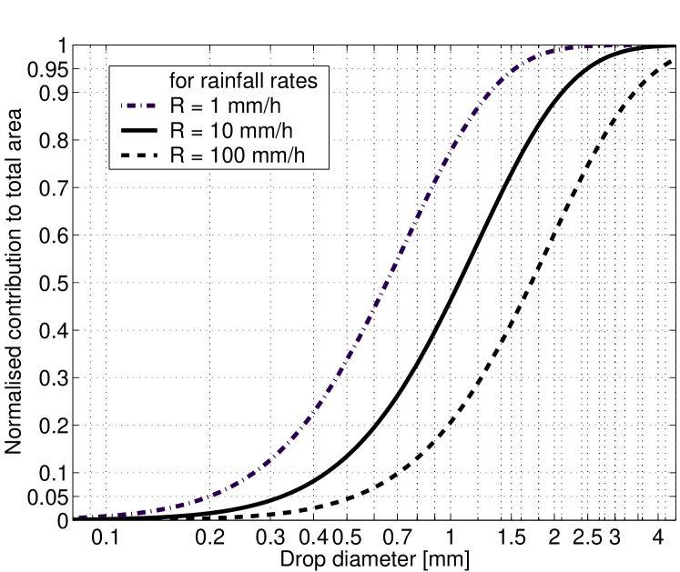
Fig. 13: Area presented to the incident light with drop diameter for three different rainfall intensities.

scatterer) for particles with $x\gg 1$, and thus

$$\tau_{z}=2\pi a^{2}N_{e}\,z$$ (22)

where the drops have again been approximated as spheres. $N_{e}$ is given by

$$N_{e}=\int\limits_{0}^{\infty}N_{0}\exp{(-\Lambda D)}\;\mathrm{d}D\,.$$ (23)

Making the substitution, we find the area-distribution from Eq. (19) in a slightly different form:

$$\tau_{z} = 2\pi N_{0}z\int\limits_{0}^{\infty}a^{2}\exp{(-\Lambda D)}\;\mathrm{d}D$$ (24)

$$= 4\pi N_{0}z\int\limits_{0}^{\infty}a^{2}\exp{(-2\Lambda a)}\;\mathrm{d}a$$ (25)

$$= \frac{\pi N_{0}}{\Lambda^{3}}\,z\,.$$ (26)

Fig. 14 shows the optical depth as a function of rainfall intensity for four different path lengths. Van de Hulst${}^{\hbox{\immediate{?}}}$ argues that single scattering prevails if $\tau_{z}<0.1$; corrections for double scattering are necessary for $0.1<\tau_{z}<0.3$, and multiple scattering is observed for even larger values of $\tau_{z}$. Other sources${}^{\hbox{\immediate{\bf{?}}}}$ maintain that multiple scattering can be neglected for $\tau_{z}$ values of up to one.

B. Numerical Simulation

The rainfall event is simulated when a large volume $V$ is created above an imaginary laser beam and filled with drops according to the Marshall Palmer distribution for a given rainfall intensity. Only drops in the size range $0.2\,\mathrm{mm}\leq D\leq 8\,\mathrm{mm}$ were considered for the

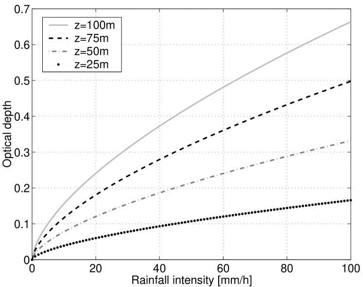
Fig. 14: Optical depth as a function of rainfall intensity for four different path lengths.

reasons outlined after Eq. (20). The total number of drops in $V$ is given by

$$N_{V}=V\,\int\limits_{0.02}^{0.8}N_{0}\exp{-\Lambda D}\;\mathrm{d}D\approx\frac{V\,N_{0}}{\Lambda}\exp{(-0.02\Lambda)}$$ (27)

with the approximation $\exp{(-0.8\Lambda)}\approx 0$ yielding negligible errors even for high rainfall intensities.

It has been shown experimentally (e.g., Ref. ${}^{\hbox{\immediate{\bf{?}}}}$) that, for a constant mean rainfall rate $R$, the number of drops is Poisson distributed around the mean. $N_{V}$ is therefore used as a mean value to produce a Poisson deviate $N_{P}$. Once the volume is filled with $N_{P}$ drops, each drop is randomly assigned a size from an exponentially weighted distribution:

$$D=-\frac{1}{\Lambda}\ln{x}\>\>\mbox{ with }\>x\in\;]0,1]$$ (28)

where $x$ is a randomly generated number. The drops are then released and fall at their terminal velocities (with the values from Gunn and Kinzer${}^{\hbox{\immediate{\bf{?}}}}$) through $V$. Every $t$ seconds a snapshot is taken, recording the number of drops present in the beam and their sizes.

C. Results

The scattering patterns are obtained when the patterns from individual drops are combined according to their abundance in the beam. The patterns from the individual drops are normalized with the cross-sectional area to obtain a constant intensity per unit area. The

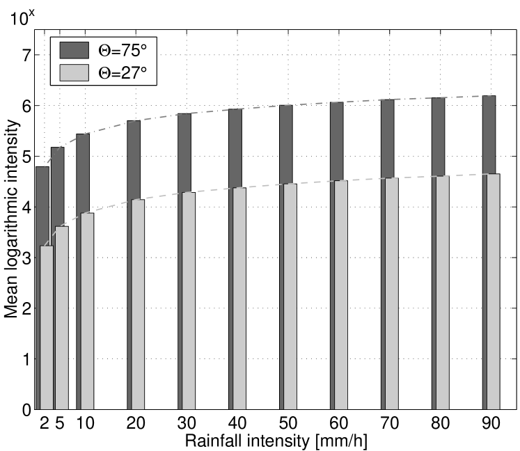
Fig. 15: Dependence of average received light intensity on rainfall rate $R$ for $(\Theta,\Phi)=(90^{\circ},75^{\circ})$ and $(\Theta,\Phi)=(90^{\circ},27^{\circ})$.

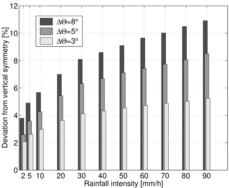
Fig. 16: Relative deviations from vertical symmetry in the scattering data for different rainfall intensities and different angular bins. The deviation is given as a percentage of the total received intensity at $(\Theta,\Phi)=(90^{\circ}$+$\Delta\Theta,90^{\circ})$.

result is a time series that gives the variations of the received intensity for each angular bin.

As expected, the results show that the higher the rainfall rate, the higher the mean scattered intensity over the sampling period. This is shown in Fig. 15 for two different angular bins. The mean detected intensity is thus a conclusive indication of the rainfall intensity $R$. The degree of asymmetry about the equator can also be used to infer the rainfall rate. Fig. 16 shows the difference between angular bins at $(\Theta,\Phi)=(90^{\circ}$–$\Delta\Theta,90^{\circ})$ and $(\Theta,\Phi)=(90^{\circ}$+$\Delta\Theta,90^{\circ})$. As can be seen, the amount of light received in the bin below the equator is considerably higher than for the corresponding element symmetrically above the equator. The difference increases as expected with rainfall intensity and varies depending on the distance to the equator.

Although the light intensity is a stable indicator of the rainfall rate, the effects of wind on the orientation of the vertical axis of the drop can be severe on the above symmetry considerations. Other factors that are likely to occur in real situations and that are neglected in this model are coalescence, drop breakup, and oscillations, as well as multiple-scattering events. Possible realizations of field experiments are given in Ref. .${}^{\hbox{\immediate{?}}}$

6. Summary

The distorted shape of raindrops at terminal velocity is often ignored and approximated with either spheres or ellipsoids. In contrast, the numerical model developed in this study determines the scattering pattern for the true drop shapes. This was achieved through a combination of geometrical optics and a statistical Monte Carlo technique. The ray trace yielded scattering patterns for different drop sizes and polarizations of the incident light. The shape of the drops could be inferred from the varying degrees of depolarization of the scattered light and the asymmetries observed in the overall scattering behavior. No experimental data are available for light scattering from distorted drops. However, the results obtained for small (spherical) drops match tabulated values confirming the validity of the model.

We have treated the problem of diffraction by successfully approximating the drops as ellipsoids. The error incurred has been found to be negligible even for the largest drops examined. Adjustments for the results from the ray trace were necessary only near the central diffraction peak whereas diffraction can be neglected for the remaining pattern.

The asymmetries in the scattering behavior can be used for rainfall measurements with a laser and several detectors as the drop size distribution depends on the rainfall intensity and thus influences the overall symmetry. Further details including the experimental realization and application to high-resolution measurements of rainfall structures can be found in Ross..${}^{\hbox{\immediate{?}}}$

This model was developed as part of a Diplomarbeit (equivalent to a Master of Science project) at the Fachbereich Physik of the Freie Universität Berlin conducted in close collaboration with the Physics Department of the University of Auckland that generously provided the resources for this research.

References

- [1] P. Lenard, “Über Regen”, Meteor. Z. 21, 249–260 (1904), [For English translation see: Q.J.R. Meteorol. Soc. 31, 62–73 (1905).].
- [2] C. Magono, “On the shape of water drops falling in stagnant air”, J. Meteor. 11, 77–79 (1954).
- [3] H.R. Pruppacher and K.V. Beard, “A wind tunnel investigation of the internal circulation and shape of water drops falling at terminal velocity in air”, Q.J.R. Meteorol. Soc. 96, 247–256, (1970).
- [4] K.V. Beard and C. Chuang, “A new model for the equilibrium shape of raindrops”, J. Atmos. Sci. 44(11), 1509–1524 (1987).
- [5] C. Chuang and K.V. Beard,“A numerical model for the equilibrium shape of electrified raindrops”, J. Atmos. Sci. 47(11), 1374–1389 (1990).
- [6] W.J. Glantschnig and S.-H. Chen, “Light scattering from water droplets in the geometrical optics approximation”, Appl. Opt. 20(14), 2499–2509 (1981).
- [7] L.G. Kazovsky, “Estimation of particle size distributions from forward scattering data”, Appl. Opt. 23(3), 455–464 (1984).
- [8] J.A. Lock, “Ray scattering by an arbitrarily oriented spheroid. II. Transmission and cross-polarisation effects”, Appl. Opt. 35(3), 515–531 (1996).
- [9] G.S. Stamaskos, D. Yova and N.K. Uzunoglu, “Integral equation model of light scattering by an oriented monodisperse system of triaxial dielectric ellipsoids: application in ectacytometry”, Appl. Opt. 36(25), 6503–6512 (1997).
- [10] A. Macke and M. Großklaus, “Light scattering by nonspherical raindrops: Implications for lidar remote sensing of rainrates”, J. Quant. Spectrosc. Radiat. Transfer 60(3), 355–363 (1998).
- [11] O.N. Ross, Optical Remote Sensing of Rainfall Micro-Structures, Diplom thesis, Fachbereich Physik der Freien Universität Berlin, (Mar 2000), http://www.soton.ac.uk/~onr/.
- [12] A. Macke, M.I. Mishchenko, K. Muinonen and B.E. Carlson, “Scattering of light by large nonspherical particles: ray-tracing approximation versus T-matrix method”, Opt. Lett. 20(19), 1934–1936 (1995).
- [13] G.A. Shah, “Geometrical Optics and Diffraction vis-à-vis Mie theory of scattering of electromagnetic radiation by a sphere”, Astrophys. Space Sci. 193, 317–328 (1992).
- [14] H.C. van de Hulst, Light Scattering by Small Particles (Wiley, New York, 1957).
- [15] C.F. Bohren and D.R. Huffman, Absorption and Scattering of Light by Small Particles (Wiley, New York, 1983).
- [16] E. Hecht, Optics, 2nd edition (Addison-Wesley, Reading, Mass., 1987).
- [17] M. Born and E. Wolf, Principles of Optics, 6th edition (with corrections) (Pergamon Press, Oxford, 1989), pp. 395–399.
- [18] D.H. Towne, Wave phenomena (Addison-Wesley, Reading, Mass., 1967), pp. 458–464.
- [19] M. Françon, Diffraction, Coherence in Optics (Pergamon, London, 1966), pp. 36–37.
- [20] J.S. Marschall and W.K. Palmer. “The distribution of raindrops with size”, J. Meteor. 5, 165–166 (1948).
- [21] E.D. Hinkley, editor. Laser monitoring of the Atmosphere, Topics in Applied Physics, Vol. 14. (Springer, Berlin, 1976), p. 101.
- [22] J. Joss and A. Waldvogel. “Raindrop size distribution and sampling size errors”. J. Atmos. Sci. 26, 566–569 (1967).
- [23] R. Gunn and G.D. Kinzer. “The terminal velocity of fall for water drops in stagnant air”. J. Meteor. 6, 243–248 (1949).