Gauge Invariant Evaluation of Nuclear Polarization with Collective Model
Abstract
The nuclear-polarization (NP) energies with the collective model commonly employed in the NP calculations for hydrogenlike heavy ions are found to have serious gauge violations when the ladder and cross diagrams only are taken into account. Using the equivalence of charge-current density with a schematic microscopic model, the NP energy shifts with the collective model are gauge invariantly evaluated for the states in Pb81+ and U91+.
pacs:
21.60.Ev, 31.30.Jv, 12.20.DsHigh-precision Lamb-shift measurement on high-Z hydrogenlike atoms BE95 spurred a renewed interest in the quantum electrodynamical (QED) calculation of electronic atoms. Comparison of theoretical results with experimental data allows sensitive tests of QED in strong electromagnetic fields SA90 ; MO98 . In this context, the study of the nuclear-polarization (NP) effect becomes important because the NP effect, as a non-QED effect which depends on the model used to describe the nuclear dynamics, sets a limit to any high-precision test of QED.
A relativistic field-theoretical treatment of NP calculation was presented by Plunien et al. PL89 ; PL95 utilizing the concept of effective photon propagators with nuclear-polarization insertions. In these studies, only the Coulomb interaction was considered based on the argument that the relative magnitude of transverse interaction is of the order of and the velocity associated with nuclear dynamics is mainly nonrelativistic.
The effect of the transverse interaction was studied in the Feynman gauge by Yamanaka et al. YA01 with the same collective model used in PL89 ; PL95 ; NE96 for nuclear excitations. They found that the transverse contribution is several times larger than the Coulomb contribution in heavy electronic atoms before the contributions of the positive and negative energy states cancel. However, due to the nearly complete cancellation between them, the transverse effects become small and the net effect is destructive to the Coulomb contribution in both states of Pb81+ and U91+. As a result, the total NP energy almost vanishes in Pb81+.
Recently, the NP effects for hydrogenlike and muonic Pb81+ were calculated in both the Feynman and Coulomb gauges, using a microscopic random phase approximation (RPA) to describe nuclear excitations HHT02 ; HHT02a . It was found that, in the hydrogenlike atom, the NP effects due to the ladder and cross diagrams have serious gauge dependence and inclusion of the seagull diagram is indispensable to restore the gauge invariance HHT02 . In contrast, the magnitude of the seagull collection is a few percent effect in the muonic atom, although it improves the gauge invariance HHT02a .
In the present paper, we report that the nuclear collective model employed for hydrogenlike ions in NE96 ; YA01 ; PL89 ; PL95 also leads to a large violation of gauge invariance as far as the ladder and cross diagrams only are considered. Then it is shown, based on the equivalence of the transition density of the collective model and a microscopic nuclear model with a schematic interaction between nucleons, that the seagull corrections should also be calculated with the collective model in order to obtain gauge invariant NP results. The resulting gauge invariant NP energy shifts are given for the states in Pb81+ and U91+.
For spherical nuclei, the Hamiltonian of the small amplitude vibration with multipolarity is written as
| (1) |
where are the canonically conjugate momenta to the collective coordinates . The lowest vibrational modes are expected to have density variations with no radial nodes, which may be referred to as shape oscillations. The corresponding charge density operator with the multipolarity is written as
| (2) |
to the lowest order of .
The liquid drop model of Bohr (BM)Bohr52 is a simple model of such a shape oscillation obtained by considering deformation of the nuclear radius parameter while leaving the surface diffuseness independent of angle:
| (3) |
where is the nuclear radius parameter of the ground state. The radial charge density of BM is given by
| (4) |
where is a charge distribution with spherical symmetry.
If we assume that under distortion, an element of mass moves from to without alteration of the volume it occupies, i.e., the nucleus is composed of an inhomogeneous incompressible fluid, a harmonic vibration of an originally spherical surface in the nucleus is given by
| (5) |
For this model we obtain
| (6) |
This version will be hereafter referred to as the Tassie Model (TM) Tassie . In Eqs.(4) and (6), is usually taken to be equal to the ground-state charge distribution.
In either case, the motion of nuclear matter is assumed to be incompressible and irrotational, hence the velocity field is given by a velocity potential as . This implies the nuclear current defined by yields the transition multipole density of current operator
| (7) |
Note that the part does not appear in the transition density of current operator given by (7).
Therefore, in this kind of collective model, the continuity equation of charge gives
| (8) |
where is the excitation energy of the surface oscillation. Hence the transition density of current is given by
| (9) |
in terms of the transition density of charge. If we assume the uniform charge distribution , we obtain, for both BM and TM,
| (10) | ||||
| (11) |
The transition densities given by (10) and (11) have been employed in the previous NP calculations for PL89 ; PL95 ; NE96 ; YA01 . It should be mentioned that, although the surface oscillation applies to the case of the multipolarity , Eqs. (10) and (11) with give the transition densities of the giant dipole resonance given by the Goldhaber-Teller model describing the relative motion of neutrons and protons DW66 . For the monopole vibration, it is also possible to construct corresponding charge and current densities YA01 ; PL89 .
In general, the charge conservation relation between the charge and current densities is necessary but not sufficient for the gauge invariance of the NP calculation. Unfortunately, it is practically impossible to construct a model that incorporates gauge invariance explicitly in terms of the collective variables of the model. However, it is possible to evaluate the NP energy gauge invariantly with the above collective model as is shown below.
The NP calculations with the collective model assume that a single giant resonance with spin multipolarity saturates the energy-weighted strength for each isospin. In this respect, let us recall the fact that the transition densities of charge to the sum-rule saturated levels are given in terms of the ground-state charge density DF73 . This can be seen as follows. For a pair of single-particle operators and , the energy-weighted sum rule can be generalized to
| (12) |
where is the charge distribution of the ground state normalized as BM75 . When a single excited state saturates the strength, , the transition density of charge to this state is derived from the sum-rule relation (12) model independently and given by
| (13) |
If the charge distribution of the ground state is assumed to be a uniform distribution with a radius , this becomes
| (14) |
which is equal to the matrix element of the charge density operator of the collective model given by (10).
On the other hand, it is well known that the schematic RPA with a separable interaction
| (15) |
for particle-hole excitations with a degenerate particle-hole excitation energy gives a collective state , which exhausts the energy-weighted sum rule for the single particle operator :
| (16) |
where is the excitation energy of RS80 . If the ground state is assumed to be a filled major shell of the harmonic oscillator potential:
| (17) |
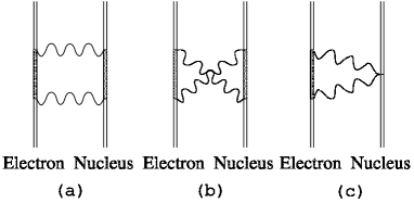
the particle-hole excitation energy is taken to be for and for and . The corresponding collective states exhaust the energy-weighted sum rules, because the transition strengths vanish outside these p-h excitation spaces. Therefore, the transition densities of charge to the collective states of this fictitious nucleus are given by (13). When the ground-state charge density is approximated by a uniform charge density, the transition density of charge becomes identical with that of the collective model employed in NP calculations for hydrogenlike atoms. However, the gauge invariant electromagnetic interaction of this schematic microscopic model is given by the minimal substitution to the Hamiltonian . Hence the lowest-order contributions to NP with this model are given by the three Feynman diagrams in Fig. 1, where two photons are exchanged between a bound electron and a nucleus. The nuclear vertices are understood to have no diagonal matrix elements for the ladder and cross diagrams, and no nuclear intermediate states for the seagull diagram. It is well known that the NP results with this model is gauge invariant provided these three diagrams are taken into account. Although current density appears in this model, dominates in the transition to the collective state.
Thus we can conclude that the gauge invariance of the collective model is also guaranteed with the charge-current density satisfying the continuity equation (8), provided the contributions from the three diagrams are taken into account. It should be noted that the seagull contribution is given in terms of the ground-state charge distribution and does not depend on the details of the model for nuclear excitations. In the actual NP calculations NE96 ; PL89 ; PL95 ; YA01 with the collective model, the assumption that each nuclear intermediate state saturates the sum-rule is not strictly obeyed, because the observed nuclear data are used for the low-lying states. However, since the gauge violation is serious only in the dipole giant resonance, this does not invalidate our arguments as is confirmed by the numerical results in the following.
The formulas to calculate the NP energy shifts due to the three diagrams of Fig. 1 were given in HHT02 for arbitrary nuclear models. In the present NP calculations of the states in hydrogenlike Pb and U, the parameters of the collective model are the same as those given in Refs. NE96 ; YA01 . The same low-lying states and giant resonances are taken into account. In addition, the contributions from the and giant resonances are also calculated in order to see the effects of higher multipoles neglected previously. The values are adjusted to the observed values for low-lying states and the are estimated through the energy-weighted sum rule for giant resonances.
Tables I and II show the results for the states in Pb81+ and U91+, where the sum of the contributions from the three diagrams of Fig.1 is given for each multipole. The second and the third columns are the results including the transverse effects in the Feynman and Coulomb gauges, respectively. The values in the parentheses are the contributions from the seagull diagram. The NP energy shifts due to the ladder and crossed diagrams only are obtained by subtraction of the seagull contributions given in the parentheses. The fourth column gives the results of the present Coulomb nuclear polarization (CNP). The last two columns are the results of the previous calculations.
| present work | Ref. YA01 | Ref. NE96 | |||||
|---|---|---|---|---|---|---|---|
| Feynman(NP) | Coulomb(NP) | CNP | NP | CNP | |||
| -3.3 | (-0.2) | -3.3 | (+0.0) | -3.3 | -6.6 | -3.3 | |
| -22.1 | (-42.3) | -21.5 | (-7.3) | -17.0 | +16.3 | -17.6 | |
| -5.8 | (+0.3) | -5.8 | (+0.6) | -5.8 | -7.0 | -5.8 | |
| -2.7 | (+0.2) | -2.8 | (+0.2) | -2.9 | -2.9 | -2.6 | |
| -1.0 | (+0.1) | -1.0 | (+0.1) | -1.1 | |||
| -0.5 | (+0.1) | -0.6 | (+0.0) | -0.6 | |||
| total | -35.4 | (-41.8) | -35.0 | (-6.4) | -30.7 | -0.2 | -29.3 |
| present work | Ref. YA01 | Ref. NE96 | |||||
|---|---|---|---|---|---|---|---|
| Feynman(NP) | Coulomb(NP) | CNP | NP | CNP | |||
| -9.3 | (-0.4) | -9.3 | (+0.0) | -9.3 | -21.5 | -9.5 | |
| -54.3 | (-65.7) | -52.5 | (-3.9) | -41.6 | -3.8 | -42.4 | |
| -131.6 | (+0.0) | -131.7 | (+1.6) | -131.6 | -148.2 | -138.9 | |
| -6.5 | (+0.3) | -6.5 | (+0.4) | -6.7 | -7.3 | -6.8 | |
| -2.0 | (+0.2) | -2.0 | (+0.2) | -2.1 | |||
| -1.0 | (+0.1) | -1.0 | (+0.1) | -1.1 | |||
| total | -204.7 | (-65.5) | -203.0 | (-1.6) | -192.4 | -180.8 | -197.6 |
The results with the collective model, as with the microscopic RPA model HHT02 , also lead to large violations of gauge invariance if ladder and crossed diagram contributions only are considered. The seagull corrections are considerable in the contributions for both of Pb81+ and U91+. Note that, in the limit of point nucleus, which is not unrealistic even for heavy hydrogenlike ions, the seagull collection occurs only in the dipole mode which involves the current density .
In Pb81+, the contributions from low-lying states are about 10% of the total results and the NP energy shift is mainly determined by the giant resonance contributions. The most dominant contribution comes from the giant dipole resonance, where a large violation of gauge invariance occurs if the seagull contributions in the parentheses are neglected: meV becomes meV and meV in Feynman and Coulomb gauges, respectively. The column 5 gives the previous results in the Feynman gauge without seagull contributions. The differences between the two results in the Feynman gauge without seagull contribution come from the accuracy of numerical integration over the continuum threshold region of electron intermediate states and from the differences of the electron wave functions: here we have used wave functions in a finite charge distribution, while YA01 employs point Coulomb solutions.
In U91+, the dominant contribution comes from the lowest excited states with a large value. Since the transition density of current in the present model given by (11) is proportional to the excitation energy, the transverse contribution of the lowest is negligible due to its exceptionally small excitation energy keV. Apart from this large Coulomb contribution, the contributions from other states show similar tendencies as in Pb81+. Namely, the contributions from other low-lying states are small compared with the giant resonance contributions, and a large gauge violation occurs in the giant dipole resonance when the seagull contribution is omitted.
To summarize, the transverse effects with the collective model are estimated gauge invariantly by inclusion of the seagull contribution. The gauge invariance is satisfied to a few percent levels in both Pb81+ and U91+ for each of the multipoles separately. Without the seagull correction, the Feynman gauge in particular does not give reliable predictions of NP, although numerical calculation in this gauge is easier than in the Coulomb gauge. Hence the conclusion of YA01 on the transverse effects is no longer tenable. The NP energy shifts are meV in Pb81+ and meV in U91+ for Coulomb (Feynman) gauge. The net transverse effect is about of the Coulomb energy shift of meV in Pb81+. This is similar to the conclusion of the microscopic model HHT02 , and should be compared with the transverse effect of the state in muonic Pb, which is about 6 % of the Coulomb contribution HHT02a . The agreement between the two models provides stability of the prediction of the NP effects with respect to the choice of the nuclear models. The percentage of the transverse effect in the total shift in U91+ is reduced to about % of the Coulomb effect due to the dominant Coulomb contribution from the lowest state.
The authors wish to acknowledge Prof. Y. Tanaka for generous support and useful discussions during our research on NP effects. They appreciate Drs. N. Yamanaka and A. Ichimura for collaboration on the NP effects with the collective model, which motivated the present work.
References
- (1) H. F. Beyer, G. Menzel, D. Liesen, A. Gallus, F. Bosch, R. Deslattes, P. Indelicato, Th. Stöhlker, O. Klepper, R. Moshammer, F. Nolden, H. Eickhoff, B. Franzke, and M.Steck, Z. Phys. D: At., Mol. Clusters 35, 169 (1995).
- (2) J. R. Sapirstein and D. R. Yennie, in Quantum Electrodynamics, edited by T. Kinoshita (World Scientific, Singapore 1990), p. 560.
- (3) P. J. Mohr, G. Plunien and G. Soff, Phys. Rep. 293, 227 (1998).
- (4) G. Plunien, B. Müller, W. Greiner, and G. Soff, Phys. Rev. A 39, 5428 (1989); 43, 5853 (1991).
- (5) G. Plunien and G. Soff, Phys. Rev. A 51, 1119 (1995); 53, 4614(E) (1996).
- (6) A. V. Nefiodov, L. N. Labzowsky, G. Plunien, and G. Soff, Phys. Lett. A 222, 227 (1996).
- (7) N. Yamanaka, A. Haga, Y. Horikawa, and A. Ichimura, Phys. Rev. A 63, 062502 (2001).
- (8) A. Haga, Y. Horikawa, and Y. Tanaka, Phys. Rev. A 65, 052509(2002).
- (9) A. Haga, Y. Horikawa, and Y. Tanaka, Phys. Rev. A 66, 034501(2002).
- (10) A. Bohr, Kgl. Dan. Vidensk.Selsk. Mat. Fys. Medd. 26, No.14 (1952)
- (11) L. J. Tassie, Austr. J. Phys. 9, 407 (1956); H. Überall, Electron Scattering from Complex Nuclei (Academic Press, New York and London, 1971), Part B, p. 573.
- (12) T. deForest, Jr. and J. D. Walecka, Adv. Phys. 15, 1 (1966)
- (13) T. J. Deal and S. Fallieros, Phys. Rev. C7, 1709(1973)
- (14) A. Bohr and B. R. Mottelson, Nuclear Structure (Benjamin, New York, 1975), Vol. 2, p. 399.
- (15) P. Ring and P. Schuck, The Nuclear Many-body Problem (Springer-Verlag, Berlin Heidelberg New York, 1980), p. 319.