‘Flat Phase’ Loading of a Bose-Einstein Condensate into an Optical Lattice

Abstract

It has been proposed that the adiabatic loading of a Bose-Einstein Condensate (BEC) into an optical lattice via the Mott-insulator transition can be used to initialize a quantum computer [D. Jaksch, et al., Phys. Rev. Lett. 81, 3108 (1998)]. The loading of a BEC into the lattice without causing band excitation is readily achievable; however, unless one switches on an optical lattice very slowly, the optical lattice causes a phase to accumulate across the condensate. We show analytically and numerically that a cancellation of this effect is possible by adjusting the harmonic trap force-constant of the magnetic trap appropriately, thereby facilitating quick loading of an optical lattice for quantum computing purposes. A simple analytical theory is developed for a non-stationary BEC in a harmonic trap.

I Introduction

Experimental advances in manipulating and controlling Bose-Einstein Condensates (BECs) of dilute atomic gases has resulted in a remarkable series of experiments Anglin . One theoretical proposal for quantum computing using atoms as qubits is to first load the atoms that are in a BEC into an optical lattice. Then, by varying the intensity of a laser used to form an optical lattice the BEC will undergo a quantum phase transition from its BEC-like superfluid state to a Mott-insulator state Jaksch . This has recently led to a seminal experiment by Bloch and collaborators Greiner .

In principle, starting with a BEC in a trap and turning on an optical lattice of sufficient well depth in a sufficiently adiabatic manner will prepare the Mott-insulator state. In practice, it is easy to turn on the optical lattice adiabatically with respect to band excitation (excitation from one band to another); however, it is substantially more difficult to turn on the optical lattice adiabatically with respect to quasi-momentum excitation. The second, more stringent form of adiabaticity requires that the optical lattice be switched on slowly with respect to mean-field interactions and tunneling dynamics between optical lattice sites, and hence typically requires milliseconds Band_02 . We will refer to the first form of adiabaticity as ‘interband adiabaticity’ and the second form as ‘intraband adiabaticity’. The intraband adiabaticity condition has been demonstrated in one-dimensional lattices by Orzel et al. Orzel and ultimately led to the pioneering experimental demonstration of the Mott-insulator transition Greiner . When not otherwise specified, the terms adiabatic and nonadiabatic in this article will refer to intraband adiabaticity.

The goal of the present paper is to present a simple strategy for remaining in the adiabatic regime while switching on the optical lattice much faster than the millisecond time scales ordinarily required for intraband adiabaticity. The strategy is to counterbalance the switching on of the optical lattice with an appropriate change in the force constant of the trap. This strategy is shown to correct and prevent much of the quasi-momentum excitation and resulting phase damage that arises from the nonadiabatic nature of the switching.

More specifically, the switching on of an optical lattice potential can divide a BEC into many individual pieces where phase coherence is maintained across the whole condensate. This phase coherence can be seen by instantaneously dropping the lattice and looking at the momentum distribution through time of flight measurements. However, because of a spatially dependent change in the density and thus the mean-field per well site, one can end up with a quadratic phase dependence developing along the lattice direction if one does not load the lattice adiabatically with respect to quasi-momentum excitations Band_02 . Elsewhere Sklarz02.1 it has been shown, using optimal control methods, that one can control the phase evolution to obtain a flat phase at some final time by time varying the harmonic trap force-constant of a confining external (typically magnetic) trap. Here we show analytically and numerically that a complete cancellation of the phase development is possible by appropriately adjusting the external trap.

This paper will focus solely on one-dimensional lattices, considering only the dynamics of the BEC along the lattice, and will ignore effects transverse to the lattice. It should be noted that the effects of transverse excitation will show-up on time scales inversely proportional to $\omega_{\perp}$ the transverse trapping frequency which is typically long compared to the times in the present paper. Work is now in progress toward further extending these results to two- and three-dimensions. It is expected BTM_02 that the squeezing of the BEC into the transverse directions can also be treated using the above method, namely by an appropriate adjustment of the trap in those directions.

There have been a number of recent publications of both experimental Pedri_01 ; Arimondo_01 ; Denschlag_02 and theoretical Stringari_02 ; BTM_02 studies involving the loading of BECs in one-dimensional lattices, and the resulting dynamics. This paper is related to these publications but focuses explicitly on a means of quickly loading an optical lattice from a BEC for quantum computing purposes, as well as for improving experimental signal to noise in short time experimental studies of BECs. Note that we consider the regime where the density of the condensate is sufficiently large that mean-field effects are not entirely negligible. Experiments can be carried out in the truly dilute gas regime where mean-field effects are negligible Denschlag_02 . However, reducing the condensate density to such low values would have to be carried out adiabatically, adversely affecting the time to load the optical lattice from the initial (dense) BEC.

The outline of the paper is as follows: in section II we define the problem. In Sec. III.1, a simple analytical theory is developed for a nonstationary 1D BEC in a harmonic trap. It is shown that a change in the density of the condensate induces a time-varying phase across the condensate that can be eliminated by a change in the harmonic force constant of the trap. In section III.2 it is shown that the effect of switching on the optical lattice is to generate a new effective normalization of the BEC and an analytical expression is obtained for the modified harmonic trap force-constant that compensates for the new effective normalization. The analytical theory is in excellent agreement with numerical simulations. A modified version of the theory in the regime where the nonlinear interaction is strong and hence the the width of the condensate differs from well to well is developed in Sec. III.3. Section IV contains the conclusion.

II Description of Problem

We consider a 1D BEC confined by a harmonic trap and governed by the Gross-Pitaevskii equation

$$i\hbar{\partial\over\partial t}{|{\psi}\rangle}=(\hat{K}+\hat{V}+NU_{0}|\psi|^{2}){|{\psi}\rangle},$$ (1)

where $\hat{K}=-{\hbar^{2}\over 2m}{\partial^{2}\over\partial x^{2}}$ is the kinetic energy operator, $\hat{V}$ is the external potential energy operator to be discussed shortly and $NU_{0}$ is the nonlinear atom-atom interaction strength, $N$ being the number of atoms and $U_{0}=4\pi a_{0}\hbar^{2}/m$ is the atom-atom interaction strength that is proportional to the $s$-wave scattering length $a_{0}$. The BEC is initially in the ground state of the trap potential and is therefore stationary. An optical lattice is then switched on, having the effect of separating the BEC wave packet into a series of localized pieces. The potential energy operator therefore takes the form $\hat{V}(x,t)={1\over 2}m\omega_{t}^{2}x^{2}+S(t)V_{0}\cos^{2}(kx)$, where $\omega_{t}$ is the trap frequency - which may be time dependent, $k$ is the laser field wave number, $V_{0}$ is the lattice intensity and $S(t)$ is the function that switches-on the laser for the optical lattice and goes from $S=0$ at the beginning of the ramp-on of the optical potential to $S=1$ at the end of the switching on time $\delta t_{s}$. In applications to quantum computing, one often wants to create an optical lattice with one atom per lattice site which will serve as quantum bits. However, due to the nonlinearity of the equations, the condensate wave function develops a phase that varies from lattice site to lattice site when the optical lattice is not turned on adiabatically Band_02 . Such a wave function can be represented by a superposition of quasi-momentum states, and a superposition of quasi-momentum corresponds to a higher energy state and thus cannot give rise to the Mott-insulator state. The problem we address is the elimination of this phase profile by adjusting the trap strength. In the coming section we analyze the evolution of BEC wave functions in harmonic traps, and consider the effect of switching on the optical lattice. Finally, a closed form for the precise time dependence of the trap strength that will insure a flat phase for the wavefunction for all times after the optical potential is fully turned on is derived.

First, however, we transform the NLSE to dimensionless units $t\to t/t_{0}$, $x\to x/x_{0}$ and $\psi\to\sqrt{x_{0}}\psi$ where for convenience we choose $t_{0}={mx_{0}^{2}\over 2\hbar}$. Performing these transformations we end up with a dimensionless NLSE

$$i{\partial\over\partial t}\psi(x,t)=\left(-{1\over 4}{\partial^{2}\over\partial x^{2}}+K(t)x^{2}+S(t)V\cos^{2}(kx)+U|\psi|^{2}\right)\psi,$$ (2)

where the trap force-constant $K=\omega_{t}^{2}t_{0}^{2}$, the field intensity $V=V_{0}{t_{0}/\hbar}$ and the nonlinear coefficient $U=NU_{0}t_{0}/x_{0}\hbar$, such that all space, time and energy quantities are now expressed in units of $x_{0}$, $t_{0}$ and $\hbar/t_{0}$ respectively.

III Analytical Theory

III.1 Dynamics of a Thomas-Fermi BEC in an Harmonic trap

Consider a normalized Thomas-Fermi type BEC wave function in a harmonic potential of the form

$$\psi(x,t)=\left\{\begin{array}[]{lll}\sqrt{3\over 4w}\sqrt{1-{x^{2}\over w^{2}}}e^{i(bx^{2}+c)}&&(x/w)^{2}\leq 1\\ 0&&(x/w)^{2}>1\end{array}\right.,$$ (3)

where the width $w(t)$ and phase components $b(t)$ and $c(t)$ are all assumed to be time dependent. We wish to analytically describe the evolution of this wave function in a harmonic trap with trap force-constant $K$ (we first consider the case where $K$ is constant in time, but the equations of motion for $w(t)$, $b(t)$ and $c(t)$ remain valid even if $K$ varies with time). Inserting the above wave function into the dimensionless NLSE, we obtain, by considering separately the real and imaginary parts, two equations involving the three parameters $w(t)$, $b(t)$ and $c(t)$. The imaginary part yields

$$-{\dot{w}\over 2w}(1-{2x^{2}\over w^{2}\alpha^{2}})=-{b\over 2}(1-{2x^{2}\over w^{2}\alpha^{2}})\quad\Rightarrow\dot{w}=wb,$$ (4)

where $\alpha\equiv\sqrt{1-{x^{2}\over w^{2}}}$, and from the real part we get

$$-\dot{b}x^{2}-\dot{c} = {1\over 4w^{2}\alpha^{4}}+b^{2}x^{2}+Kx^{2}+U{3\over 4w}(1-{x^{2}\over w^{2}})$$ (5)

$$\approx {1\over 4w^{2}}(1+{2x^{2}\over w^{2}})+(b^{2}+K)x^{2}+U{3\over 4w}(1-{x^{2}\over w^{2}}).$$

In going to the last line we expanded ${1\over\alpha^{4}}$ in a Taylor series in $x/w$, truncating after the second order. Comparing separately the coefficients of $x^{0}$ and $x^{2}$, we obtain the following two equations of motion for $b(t)$ and $c(t)$:

$$\dot{b} = -{1\over 2w^{4}}+{3U\over 4w^{3}}-(b^{2}+K),$$ (6)

$$\dot{c} = -{1\over 4w^{2}}-{3U\over 4w}.$$ (7)

Taking a time derivative of Eq. (4) and using Eq. (6) we find

$$\ddot{w} = \dot{b}w+b\dot{w}$$ (8)

$$= -{1\over 2w^{3}}+{3U\over 4w^{2}}-Kw$$

$$\equiv -{\partial\over\partial w}V_{e}(w),$$

with the effective potential $V_{e}(w)$ defined as

$$V_{e}(w)\equiv-{1\over 4w^{2}}+{3U\over 4w}+{1\over 2}Kw^{2}.$$ (9)

The time evolution of the wave function width, $w$, can therefore be easily determined by considering the form of the potential $V_{e}(w)$. Furthermore, by defining

$$p\equiv wb,$$ (10)

we can formulate the equations for the conjugate variables $w$ and $p$ as a Hamiltonian system of equations with $H(w,p)=p^{2}/2+V_{e}(w)$ such that

$$\dot{w} = {\partial\over\partial p}H=p$$ (11)

$$\dot{p} = -{\partial\over\partial w}H=-{\partial\over\partial w}V_{e}.$$ (12)

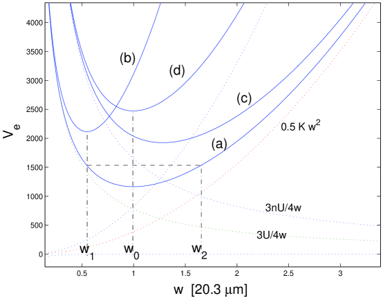
Figure 1: a) $V_{e}(w)$ with stationary point $w_{0}$ and examples of turning points $w_{1}$ and $w_{2}$ marked. The asymptotic curves correspond to the contributions of the two dominant terms in $V_{e}$ and highlight the way changes in these terms effect the dynamics. b) $V_{e}^{\prime}$ chosen such that $w_{0}^{\prime}=w_{1}$ by adjusting $K$. c) $V_{e}^{\prime}$ obtained from (a) as a consequence of change in wave function normalization. d) a new $V_{e}^{\prime}$ obtained from (c) by also changing $K$ to compensate for the change affected by the normalization change shown in (c).

Consider now the potential $V_{e}(w)$ in (9) plotted as curve (a) in Fig. 1. The potential consists of a well centered around the stable point $w_{0}\approx({3U\over 4K})^{1\over 3}$. This can be most easily obtained by setting $b=0$ and $\dot{b}=0$ in Eq. (6) and solving for $w$ while noticing that the first term on the RHS of (6) is small compared to the rest and can therefore be neglected. With initial wave function width $w(0)=w_{0}$, where $w_{0}$ is the width of the Thomas-Fermi stationary ground state of the trap, the wave function will remain stationary throughout. However, if the initial width equals some other value, an oscillatory motion of $w$ round the stationary point $w_{0}$ will develop. The phase curvature $b$ will also oscillate with $w$ obtaining its maximum value when $w(t)=w_{0}$ and vanishing when $w$ approaches its turning points, $w_{1}$ and $w_{2}$.

If an abrupt change in the trap force-constant can be made, $K\to K^{\prime}$, at the exact point in time when $b(t)=0$, i.e., when $w(t)$ is at one of its turning points, e.g., $w=w_{1}$, then it is possible to change the potential so as to freeze the flat phased wave function and make it stationary. This can be obtained by choosing $K^{\prime}={3U\over 4w_{1}^{3}}$ such that $w_{1}$ is the stationary point of the new potential $V_{e}^{\prime}$ (curve (b) in Fig. 1).

Another scenario to be considered is the following. We begin with a stationary flat phased wave function residing at the stationary point $w_{0}$ of the potential. Imagine now the hypothetical possibility of abruptly changing the normalization of the BEC wave function from unity to $n$. This would be equivalent to a change in the potential $V_{e}\to V_{e}^{\prime}$ affected by changing $U\to nU$. It is obvious that this change will shift the stationary point to some new value $w_{0}^{\prime}=({3nU\over 4K})^{1\over 3}$ (see curve (c) in Fig. 1) and that the wave function currently positioned at $w_{0}$ will no longer be stationary under the new potential. In order to compensate for this change and keep the wave function stationary one can adjust the trap force-constant and set $K^{\prime}=nK$ such that ratio $U/K$ remains constant and the stationary point $w_{0}^{\prime}=w_{0}$ will not shift (see curve (d) in Fig. 1).

We show in the following section that turning on an optical lattice corresponds to a change in the normalization of the wave function, so that the above scenario corresponds precisely to our goal of achieving a flat phased BEC loading of an optical lattice. It should be noted that the above analysis ignores gravity which can be assumed to be orthogonal to the lattice direction. However, even if gravity is along the lattice direction a similar analysis holds but requires an additional linear offset.

III.2 Switching on the Optical Lattice

Quickly switching on the optical lattice causes the BEC wave function, which initially has a Thomas-Fermi form of an inverted harmonic potential, to split into a series of localized pieces each residing in a lattice well. As the overall normalization of the wave function must remain unity, the displaced population from areas between the lattice wells builds up within the wells such that the density in these regions increases dramatically (see Fig. 2). However, if we neglect the local lattice structure and consider solely the global nature of the BEC wave function, we see that it retains its quadratic shape, and the change in the wave function brought about by the existence of the optical lattice can be viewed as a stretching of the Thomas-Fermi wave function in the vertical direction (see Fig. 2). This picture is based on a separation of scales in the spatial dimension which is a consequence of the fact that the length of each lattice well, ${\lambda\over 2}={\pi\over k}$, is much smaller than the scale of the total wave packet, $w$ (see for example Ref. Stringari_02 ). It is for this reason that we can treat first the local structure of the wave function in each well and then consider separately the overall global evolution of the wave function.

The idea is therefore to view the wave function on a level coarser than the lattice site dimension, averaging out the local lattice structure of the wave function. This procedure yields a new Thomas-Fermi type wave function $|\psi_{\mathrm{glob}}|^{2}={\langle{|\psi|^{2}}\rangle}_{\mathrm{loc}}={3n\over 4w}{(1-{x^{2}\over w^{2}})}$ differing from the initial one by a modified normalization factor $n$ (see Fig. 2). The evolution of this wave function can then be analyzed using the results of the previous section.

This procedure can also be viewed as a spatial-averaging out of the local structure of the Hamiltonian operator ${\langle{H}\rangle}_{\mathrm{loc}}={\langle{T+V_{\mathrm{lattice}}+V_{t}+U|\psi|^{2}}\rangle}_{\mathrm{loc}}=T^{\mathrm{av}}+V^{\mathrm{av}}_{\mathrm{lattice}}+V_{t}+U{\langle{|\psi|^{2}}\rangle}_{\mathrm{loc}}$. The harmonic trap potential $V_{t}$ is constant on the local scale and is therefore unaffected by the averaging. If the average kinetic and lattice potential energies per particle, $T^{\mathrm{av}}$ and $V^{\mathrm{av}}_{\mathrm{lattice}}$, are constant from well to well, these contributions to the energy can be absorbed into the chemical potential $\mu$, resulting in just the averaged global mean-field playing-off, on the global scale, against the trap potential as in a simple Thomas-Fermi procedure. The trap must then be adjusted to compensate only for the varying mean-field across the BEC wave function.

In obtaining this simplified picture we distinguish between two opposite scenarios occurring on the local scale. In many cases, when considering the dynamics along the direction of the one-dimensional lattice, the mean-field within each well is negligible in comparison with the kinetic and potential energies along this direction. This occurs for tight optical wells, e.g., short wavelength and strong intensity such that $\sqrt{V}k^{2}\gg U/w$, where $w$ is the width of the BEC. The local wave function can then be well approximated by a Gaussian with a “well-independent” width implying that the locally averaged kinetic and lattice potential energies are also “well-independent”. In carrying out the above procedure we then find that the global wave function is a stretched image of the initial one, as described above.

In the opposite regime the mean-field within each well can no longer be neglected. In these cases the calculations are more involved and do not yield the simplified picture presented here of a mere stretching of the wave function. Instead, a distortion occurs which must be treated explicitly. We therefore delay discussion of this scenario and provide a more general treatment in the next section.

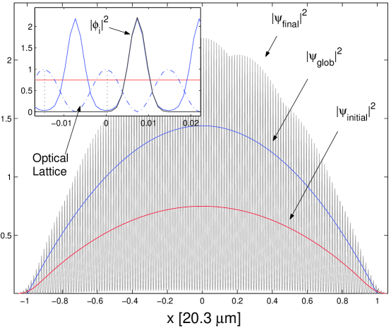
Figure 2: Analysis of the BEC wave function in an optical lattice. $\psi_{init}$ and $\psi_{final}$ are the wave functions before and after applying the optical lattice, and $\phi_{i}(x)$ is the local wave function within a specific well. (Gaussian approximation) $\psi_{\mathrm{glob}}$ is the global Thomas-Fermi type wave function after averaging out the local details.

In the following we wish to determine the normalization factor $n$ in terms of the optical lattice parameters $V$ and $k$. Consider the initial Thomas-Fermi wave function $|\psi|^{2}={3\over 4w}(1-{x^{2}\over w^{2}})$. The number of atoms in the region of each lattice well determined by its position $x_{i}$ is

$$\eta(x_{i}) = |\psi(x_{i})|^{2}{\lambda\over 2}$$ (13)

$$= {3\pi\over 4wk}(1-{x_{i}^{2}\over w^{2}}).$$

Assuming that the local population becomes trapped in the well during the switching on of the optical lattice, we can then consider the local normalization factor per well as constant throughout the evolution. Assuming too that the wave function at each lattice site is localized after the optical lattice has been switched on, we can ascribe to each lattice site a local wave function, $\phi_{i}(x)$, which is normalized to $\eta_{i}$. In order to obtain an average norm per well we define the local probability function $P_{i}(x)$ which is just the local wave function normalized to unity

$$P_{i}(x)={1\over\eta_{i}}|\phi_{i}(x)|^{2}.$$ (14)

Averaging out the local structure using the local probability function, $P_{i}(x)$, we obtain the coarse-grained wave function,

$$|\psi_{\mathrm{glob}}(x_{i})|^{2}={\langle{|\phi_{i}|^{2}}\rangle}_{\mathrm{loc}} = \int P_{i}(x)|\phi_{i}(x)|^{2}dx$$ (15)

$$= {1\over\eta_{i}}\int|\phi_{i}(x)|^{4}dx.$$

Note, the limits of integration in the above integral should be restricted to a single well but due to the gaussian-like nature of the wavefunction $\phi_{i}(x)$ the specific limits are unimportant. Note that in evaluating the integral, $\eta_{i}$ was considered constant as it is only slowly varying on the local scale.

In many cases the local wave function can be well approximated by a Gaussian

$$\phi_{i}(x)=\sqrt{\eta_{i}\over\pi^{1/2}\Delta}e^{-{(x-x_{i})^{2}\over 2\Delta^{2}}}e^{i\Phi},$$ (16)

where $\Delta$ is the width and the wave function normalizes to the local normalization factor $\eta_{i}$ (see inset in Fig. 2). $\Delta$ is of typically on the order of but smaller than $\lambda\ll w$ and is therefore small compared with the width of the total wave function, so $\eta(x_{i})$ is only slowly varying with respect to $x$ and can be considered constant within any given lattice site. Averaging out the local structure we obtain the coarse wave function $\psi_{\mathrm{glob}}(x_{i})$ which we now show to be of Thomas-Fermi type

$$|\psi_{\mathrm{glob}}(x_{i})|^{2} = {\langle{|\phi_{i}|^{2}}\rangle}_{\mathrm{loc}}=\int P_{i}(x)|\phi_{i}(x)|^{2}dx$$ (17)

$$= {\eta_{i}\over\sqrt{\pi}\Delta}{1\over\sqrt{\pi}\Delta}\int e^{-2{(x-x_{i})^{2}\over\Delta^{2}}}dx$$

$$= {\eta_{i}\over\sqrt{2\pi}\Delta}$$

$$= {3\over 4w}\sqrt{\pi\over 2}{1\over k\Delta}(1-{x_{i}^{2}\over w^{2}})$$

$$\equiv {3n\over 4w}(1-{x_{i}^{2}\over w^{2}}).$$

In going from the third to the fourth line we used the explicit form of $\eta_{i}$ given in (13). Comparing the last two lines we find the modified normalization to be

$$n=\sqrt{\pi\over 2}{1\over k\Delta}.$$ (18)

It remains to determine the local width $\Delta$ of the wave function within each lattice site in terms of the external parameters. It can be shown analytically (see appendix A) that

$$\Delta=\sqrt{-{2\over k^{2}}\mathcal{W}(-{k\over 4\sqrt{V}})}$$ (19)

where $\mathcal{W}(x)$ is the Lambert W function LambertW , so that the normalization factor $n$ is finally given by

$$n={1\over 2}\sqrt{-\pi\over\mathcal{W}(-{k\over 4\sqrt{V}})}.$$ (20)

The effect of switching on the optical lattice on the dynamics of the wave function can now be viewed as changing the normalization of the initial wave function from unity to $n$.

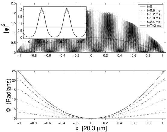
Figure 3: Evolution of the wave function (amplitude and phase) as a consequence of switching on the optical lattice. Note the development of a quadratic phase profile.

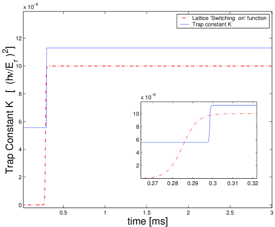
Figure 4: Sequence of external fields keeping phase of wave function flat and stationary.

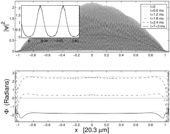
Figure 5: Evolution of the wave function (amplitude and phase) as a consequence of switching on the optical lattice and adjusting the compensating trap force-constant. The stationary flat phase is strikingly apparent.

If the switching-on time $\delta t_{s}$ is short compared to the global nonlinear time scale $t_{NL}$ Trippenbach00 so as no substantial phase evolution occurs during this time, the transformation of the normalization constant can be considered abrupt and the dynamics of the wave function parameters $w(t)$ and $b(t)$ are raised from the initial potential curve $V_{e}$ to $V_{e}^{\prime}$ (curves (a) and (c) respectively in Fig. 1) by the change $U\to nU$ as described in the previous section. If no further adjustments are made, the wave function will begin to evolve on the potential curve $V_{e}^{\prime}$ and develop phase as seen in Fig. 3. In order to cancel this effect one can compensate for the change of normalization by adjusting the trap force-constant to $K=nK_{0}$ (curve (d) of Fig. 1). In Fig. 4 we plot the switching-on function of the optical lattice and the change of the trap force-constant $\Delta K=K-K_{0}$ as a function of time. The evolution of the wave packet under this sequence of events is plotted in Fig. 5, from which it is evident that the phase remains constant throughout the evolution for the correct tuning of the trap force-constant.

In the simulations presented here we have taken $N=1.5\times 10^{6}$ sodium atoms, a scattering length of $a_{0}=2.8$ nm, and a trap of average frequency $59.26$ Hz. Using these values the Thomas-Fermi approximation to the chemical potential, $\mu_{\mathrm{TF}}$, can be calculated and the nonlinear interaction time becomes $t_{NL}\equiv{\hbar/\mu_{\mathrm{TF}}}=96.2\,\mu$s. In order to preserve the time scales in the 1D model as they are in 3D reality, we follow Ref. Trippenbach00 and replace the nonlinear coefficient $NU_{0}$ by $C\mu_{\mathrm{TF}}x_{\mathrm{TF}}$, where the Thomas-Fermi radius $x_{\mathrm{TF}}=\sqrt{{2\mu_{\mathrm{TF}}/m\omega^{2}_{t}}}$ gives the size of the condensate and the factor $C$ carries the dependence of the simulation on the dimensions and is for our 1D case $C={\sqrt{\pi}\over\Gamma(2+1/2)}={4\over 3}$ Trippenbach00 .

We take the optical lattice wavelength to be $\lambda=589$ nm and choose $x_{0}=\lambda/\pi=2/k$ such that $t_{0}=\hbar/E_{r}$, where $E_{r}\equiv{\hbar^{2}k^{2}\over 2m}$ is recoil energy. The optical lattice is switched on in a time $\delta t_{s}\approx 20\mu s$ to the final intensity of $V_{0}=10.94\,E_{r}$. In units of $x_{0}=\lambda/\pi$, $t_{0}$ and $\hbar/t_{0}=E_{r}$, for space, time and energy quantities respectively, we therefore get the following unitless values; $k=2$ for the optical wave number, $K=({\hbar\omega_{t}\over E_{r}})^{2}=5.615\times 10^{-6}$ for the initial trap force-constant, $V=10.94$ for the final field intensity and $U={4\over 3}{t_{0}\over t_{NL}}{x_{\mathrm{TF}}\over x_{0}}=9.55$ for the nonlinear interaction strength.

Inserting these values into Eq. (20) yields the normalization factor $n=2.0866$ such that the trap force-constant which we analytically predict to yield an optimally flat phase is $K=1.172\times 10^{-5}$ ($85.5$ Hz). This value is off by merely $2\%$ from the empirically found optimal value of $K=1.151\times 10^{-5}$ ($84.8$ Hz) which generates the evolution plotted in Fig. 5. Some small residual spatially varying phase structure remains. This structure is due to incomplete interband adiabaticity and can be reduced by increasing the switching-on time $\delta t_{s}$.

III.3 Nonlinear Regime

We now return to the more complicated scenario where the local wave function has spatially varying contributions from the mean-field term. Various complications arise in this regime which must be solved individually. The main complication is due to the fact that when the mean-field is locally important it affects the width and shape of the local wave functions such that they differ from well to well as shown in appendix A. This implies that the average kinetic and lattice potential energies also vary from well to well, affecting the phase accumulation.

Assuming that the local wave function can still be approximated by a Gaussian along the lattice direction (as is the case unless the local mean-field is larger than the kinetic energy) we can use the results of appendix A to obtain the well-dependent width $\Delta(x_{i})$. This can be inserted back into Eq. (23) to obtain the total local energy as a sum of its contributions: the kinetic energy $T$, the lattice potential energy $E_{\mathrm{lattice}}$, the trap potential energy $E_{t}$ and the mean-field energy $E_{mf}$. The chemical potential associated with a specific lattice site is Dalfovo99

$$\mu = {1\over\eta}(T+E_{\mathrm{lattice}}+E_{t}+2E_{mf})$$ (21)

$$= {1\over 8\Delta_{i}^{2}}+{V\over 2}(1-e^{-k^{2}\Delta_{i}^{2}})+V_{t}(x_{i})+{\eta_{i}U\over\sqrt{2\pi}\Delta_{i}}.$$

In order to keep the phase evolution constant from well to well one must adjust $V_{t}(x_{i})$ such that it cancels all other $x_{i}$ dependencies (originating in $\Delta(x_{i})$ and $\eta(x_{i})$) and thus makes $\mu$ independent of $x_{i}$. Another complication arises from the fact that the optical lattice must be switched on adiabatically with respect to interband excitations (as stressed in the introduction), e.g., the switching-on time $\delta t_{s}$ in our dimensionless units must be longer than ${2\pi\over k\sqrt{V}}$. This means that for experiments in which the lattice wavelength is large, the lower bound on the switching-on time becomes comparable to $t_{NL}$ and considerable phase evolution will occur during this time.

To avoid the phase winding during the switching-on time one must make the trap frequency change gradually so as to compensate for the changing shape of the wave function at intermediate times. We assume as a zeroth order approximation that a transition of the magnetic trap from its initial to its final form using the same switching-on function as the optical lattice, will momentarily compensate for the changing shape of the wave function. The relevant parts of the potential terms in the Hamiltonian will take the following form $(1-S(t))V_{t}^{\mathrm{init}}+S(t)V_{t}^{\mathrm{final}}+S(t)V\cos^{2}(kx)$.

In Fig. 6 we show a case where the mean-field is important. In this simulation we chose parameters as above, except the optical lattice wavelength and strength were changed to be $\lambda=8\times 589$ nm, and $V_{0}=45.4\,E_{r}$ respectively so that the mean-field within each well is no longer negligible. With these parameters and following the above procedure we found the optimal trap shape to be of the form $V^{\mathrm{final}}_{t}=K\{1-(1-({x\over w})^{2})^{0.8}\}$ with $K=11.88$, where $w=x_{\mathrm{TF}}/x_{0}=13.5$ is the width of the BEC in the units of $x_{0}$ introduced above. We turned on the new trap shape gradually, as described above, with a switching-on time of $\delta t_{s}\approx 1$ ms, the resulting constant flat phase can be clearly seen in Fig. 6. Some small residual spatially varying phase structure due to incomplete interband adiabaticity remains here too, and increasing the switching-on time $\delta t_{s}$ will reduce the residual phase structure.

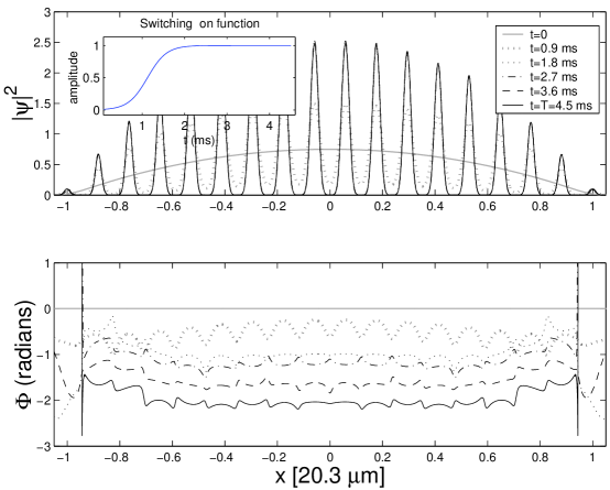
Figure 6: Evolution of the wave function (amplitude and phase) as a consequence of adiabatically switching on the optical lattice and adjusting the compensating trap (strength and shape).

IV Conclusions

The switching on of an optical lattice potential can divide a BEC into many individual pieces where phase coherence is maintained across the whole condensate. However, because of a spatially dependent change in the density and thus the mean-field per well site, one can end up with a quadratic phase dependence developing along the lattice direction if one does not load the lattice adiabatically. We have shown analytically and numerically that a cancellation of this effect is possible by appropriately adjusting the external trap. A simple analytical theory has been developed for a non-stationary 1D BEC in a harmonic trap. It was shown that the effect of switching on the optical lattice is to generate a new effective normalization of the BEC, and hence a nonstationary condensate. Finally, an analytical expression was obtained for the modified harmonic trap force-constant that compensates for the new effective normalization. The analytical theory is in excellent agreement with numerical simulations.

In real experiments more care is needed to account for the effects of evolution in the transverse directions. Work is now in progress toward extending these results to two and three dimensions. It is expected that the expansion of the BEC into the transverse directions can also be treated using the above method namely by an appropriate adjustment of the trap in those directions. We have detailed elsewhere how our quasi-1D calculations of the type we presented here model 3D aspects of the dynamics in cylindrically symmetric potentials BTM_02 , but this method can not describe radial excitations of the BEC that might arise due to the optical potential via the mean-field interaction. To the extent that radial excitations are not important, our method should be an adequate approximation to the 3D dynamics.

It is not known how a small residual spatially varying phase will affect the Mott-insulator transition. The residual phase can be thought of as a phonon-like excitation that should be mapped onto the final Mott-Insulator state. Characterizing the nature of excitations in an inhomogeneous Mott-Insulator has not been done; however, the small residual excitations seen here are not expected to have a strong effect since the total energy of the system is only slightly above that of the ideal case. A more exact answer to this question can not be provided within the context of a mean-field approach and requires analysis using many-body approaches to the Mott-insulator transition. Moreover, no theoretical model exists that is completely appropriate in both the superfluid and Mott-Insulator regimes.

Appendix A Calculation of local wave function width $\Delta$

As in the text we approximate the local wave function by a Gaussian

$$\phi_{i}(x)=\sqrt{\eta(x_{i})\over\pi^{1/2}\Delta}e^{-{(x-x_{i})^{2}\over 2\Delta^{2}}},$$ (22)

of width $\Delta$, normalized to the local normalization factor $\eta_{i}$ and centered around $x_{i}$. We wish here, using the variational method, to determine the width of the Gaussian in terms of the optical lattice strength $V$ and wave number $k$.

We first compute the energy associated with $\phi_{i}$ as a function of $\Delta$:

$$E(\Delta) = \int\phi_{i}^{*}(x)\left(-{1\over 4}{\partial^{2}\over\partial x^{2}}+V_{t}(x_{i})+V\sin^{2}(k(x-x_{i}))+{1\over 2}U|\phi_{i}(x)|^{2}\right)\phi_{i}(x)dx$$ (23)

$$= ({\eta(x_{i})\over\sqrt{\pi}\Delta})\int e^{-{(x-x_{i})^{2}\over 2\Delta^{2}}}\left(-{1\over 4}{\partial^{2}\over\partial x^{2}}+V_{t}(x_{i})+V\sin^{2}(k(x-x_{i}))+{1\over 2}U|\phi_{i}|^{2}\right)e^{-{(x-x_{i})^{2}\over 2\Delta^{2}}}dx$$

$$= \eta(x_{i})\left({1\over 8\Delta^{2}}+V_{t}(x_{i})+{V\over 2}(1-e^{-k^{2}\Delta^{2}})+{\eta(x_{i})U\over 2\sqrt{2\pi}\Delta}\right).$$

Note that the trap potential, denoted $V_{t}$ and the number of atoms in the region of the lattice well at position $x_{i}$, $\eta(x_{i})$, were extracted from the averaging integral since they are assumed constant on the local scale. According to the variational principal, the determine the ground state function, $\phi_{i}$, which minimizes the energy $E(\Delta)$ with respect to $\Delta$:

$${\partial E(\Delta)\over\partial\Delta}=\eta_{i}\left(-{1\over 4\Delta^{3}}+V\Delta k^{2}e^{-k^{2}\Delta^{2}}-{\eta_{i}U\over 2\sqrt{2\pi}\Delta}\right)=0.$$ (24)

An explicit solution of this equation for $\Delta$ is not possible in general; we therefore distinguish between several cases and make some simplifying assumptions. If, as is the case for short optical wavelength, the mean-field term becomes negligible with respect to the other energy terms, it can be neglected to obtain the following equation

$$\Delta^{4}e^{-k^{2}\Delta^{2}}={1\over 4Vk^{2}}.$$ (25)

The solution to this secular equation can be written in terms of the Lambert $\mathcal{W}$ function, $y=\mathcal{W}(x)$, which is defined as the inverse of $x=ye^{y}$ LambertW ,

$$\Delta=\sqrt{-{2\over k^{2}}\mathcal{W}(-{k\over 4\sqrt{V}})}.$$ (26)

It can be seen in the inset of Fig. 2 that this value for the width of the local wave function gives good results. An important point to note is that in this regime $\Delta$ is independent of the well position, implying that the lattice potential and kinetic energies per particle too are “well-independent”. This crucial point justifies our treatment of the global wave function $\psi_{\mathrm{glob}}$ as a Thomas-Fermi approximation.

For high density BECs and longer optical wavelengths the mean-field cannot be neglected and Eq. (24) must be numerically solved for $\Delta$. It must be noted, however, that the resulting form for $\Delta(x_{i})$ will in general be “well-dependent”, implying that the kinetic and lattice potential energies per particle will also be “well-dependent” and thus contribute to the phase curvature accumulation. This must be taken into account when adjusting the trap to counter the phase accumulation, within the non-negligible mean-field regime, as will be discussed in section III.3.

- (1) See, for example, J.R. Anglin and W. Ketterle, Nature, 416, 211 (2002), and references therein.
- (2) D. Jaksch, et al., Phys. Rev. Lett. 81, 3108 (1998).
- (3) M. Greiner, et al., Nature 415, 39 (2002).
- (4) Y.B. Band and M. Trippenbach, Phys. Rev. A 65, 053602 (2002).
- (5) C. Orzel, et al., Science 291, 2386 (2001).
- (6) S. E. Sklarz and D. J. Tannor, Phys. Rev. A (submitted).
- (7) Y. B. Band, I. Towers and B. A. Malomed, cond-mat/0207739.
- (8) P. Pedri et al., Phys. Rev. Lett. 87, 220401 (2001).
- (9) O. Morsch, J.H. Müller, M. Cristiani, D. Ciampini and E. Arimondo, Phys. Rev. Lett. 87, 140402 (2001).
- (10) J.H. Denschlag et al., J. Phys. B: At. Mol. Opt. Phys. 35, 3095 (2002).
- (11) M. Krämer, L. Pitaevskii, and S. Stringari, Phys. Rev. Lett. 88, 180404 (2002).
- (12) D. J. Jeffrey, and D. E. Knuth, “On the Lambert W Function”, Advances in Computational Mathematics, Vol. 5, pp. 329-359 (1996).
- (13) M. Trippenbach, Y.B. Band and P.S. Julienne, Phys. Rev. A 62, 023608 (2000).
- (14) F. Dalfovo, et al., Rev. Mod. Phys. 71, 463-512 (1999).