Signal detection by means of phase coherence induced through phase resetting

Abstract

Detection and location of moving prey utilizing electrosense or mechanosense is a strategy commonly followed by animals which cannot rely on visual sense or hearing. In this article we consider the possibility to detect the source of a localized stimulus that travels along a chain of detectors at constant speed. The detectors are autonomous oscillators whose frequencies have a given natural spread. The detection mechanism is based on phase coherence which is built up by phase resetting induced by the passing stimulus.

The ability to detect, locate, and capture prey is vital for survival. Many animals accomplish these tasks using visual or acoustic information. However, species that have developed in an environment where these senses are obscured, have to rely on alternative mechanisms. For example, the paddlefish (Polyodon spathula), found in the river basins of the Midwestern United States and in the Yangtze River in China, makes use of a passive electrosensory system pfish . Another example is the weakly electric fish that combines active and passive electrosense with a mechanosensory lateral line system elfish . In these animals, receptors transform stimuli into electric signals which excite the terminals of primary afferent neurons. These afferents are well known to exhibit periodic spike patterns spikepat .

In the last decades a lot of research has been devoted to the details of information processing on the neural level, i.e., the dynamics of single neurons or neural networks. However, at the behavioral level still many open problems exist. Since the performance and the analysis of experiments usually involve an enormous effort, efficient and tractable models are indispensable, both for planning and interpretation.

Here we present an idealized, however, analytically tractable model, proposing a mechanism for the detection of a localized stimulus. This stimulus is passing an array of receptors, which we model as phase oscillators. To measure the degree of coherence between the oscillators we choose the well known synchronization index synchroindex . First we examine the influence of a random initial distribution of the oscillator phases on the synchronization index and introduce a threshold value to distinguish a stimulus from a “false alarm”. Then we investigate the influence of our model parameters for the detection of a moving stimulus.

We consider a linear chain of $N$ uncoupled phase rotors which are characterized by the set of variables $\psi_{1},\ldots,\psi_{N}$. The rotors are aligned at equal distance along an axis of length $L$, i.e. the position of rotor $k$ is $x_{k}=(N-k)/(N-1)L$, $k=1,\ldots,N$. Each rotor has its own natural frequency $\Omega_{k}$ which, in the absence of a stimulus, determines the simple linear growth of the phase, i.e. $\psi_{k}(t)=\psi_{k}(0)+\Omega_{k}t$. We assume the frequencies to be independently and identically distributed according to a Gaussian with mean $\Omega_{0}$ and standard deviation $\Delta\Omega=\eta\Omega_{0}$.

An appropriate quantity to measure the degree of phase coherence among these rotors is the complex variable

$$Z(t)=\frac{1}{N}\sum_{k=1}^{N}\exp\left[i\psi_{k}(t)\right]=:R(t)\exp\left[i\Phi(t)\right].$$ (1)

This global order parameter contains both the information about the instantaneous collective phase $\Phi(t)$ and the instantaneous degree of phase coherence measured by the modulus $R(t)$ at time $t$. Its square can be expressed in several ways:

$$R^{2}(t) = \frac{1}{N^{2}}\left\{\left[\sum_{k=1}^{N}\cos(\psi_{k}(t))\right]^{2}+\left[\sum_{k=1}^{N}\sin(\psi_{k}(t))\right]^{2}\,\right\}$$ (2)

$$= \frac{1}{N^{2}}\left[\sum_{k,l=1}^{N}\cos(\psi_{k}(t)-\psi_{l}(t))\right]$$ (3)

$$= \frac{1}{N}+\frac{2}{N^{2}}\sum_{k=1}^{N}\sum_{l>k}^{N}\cos(\psi_{k}(t)-\psi_{l}(t))$$ (4)

This quantity is termed synchronization index since it is widely used in the description of synchronization processes synchroindex . From Eqs. (2) and (3) it is obvious that $0\leq R(t)\leq 1$ with $R(t)=1$ indicating perfect coherence.

We initialize the array by randomly selecting a phase for each of the rotors according to the uniform distribution on $[0,2\pi)$. Thus, the quantity $R_{0}=R(t=0)$ is a random variable. Its density contains important information because even in the absence of any signal the array of rotors will generate nonvanishing values of $R_{0}$. These have to be discriminated from values of $R(t)$ which significantly indicate coherence induced by the passing stimulus. Figure 1 shows numerically estimated densities, where $N=10,100,1000,10000$ equidistributed phases were used to compute a single realization of the random variable $R_{0}$.

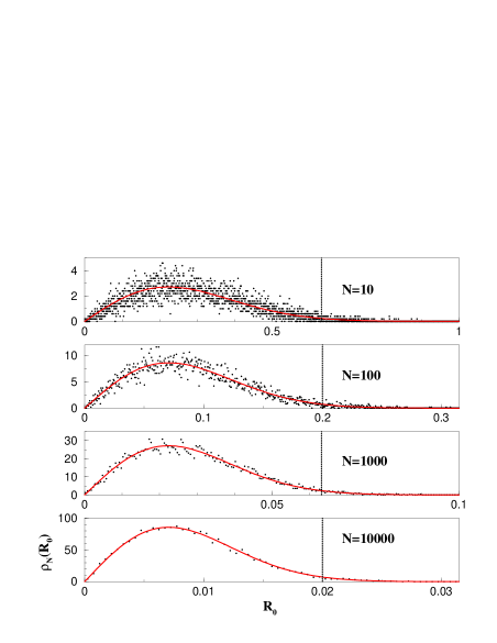
Figure 1: The density of the random variable $R_{0}$ for different $N=10,100,1000,10000$ (top down). The dots indicate the result of numerical simulations whereas the full line identifies the Rayleigh distributions (7). Vertical lines mark the threshold set by the value $2/\sqrt{N}$, which corresponds to a $2\%$ level of false alarm.

An analytic expression for these distributions can be derived by applying the central limit theorem (Lindenberg-Lévy theorem) to the following pair of random variables

$$X_{N}={1\over N}\sum_{k=1}^{N}\cos[\psi_{k}(0)]\,,\quad Y_{N}={1\over N}\sum_{k=1}^{N}\sin[\psi_{k}(0)]$$ (5)

which yields for large $N$ the limiting density Fisz

$$\rho(X_{N}=x,Y_{N}=y)\simeq{N\over\pi}\exp\left[-N(x^{2}+y^{2})\right]\,.$$ (6)

Changing to polar coordinates $(R_{0},\Phi_{0})$ and integrating over the angle $\Phi_{0}$ immediately leads to the Rayleigh distribution (Fig. 1)

$$\rho_{N}(R_{0})=2NR_{0}\exp(-NR_{0}^{2})\,.$$ (7)

Mean and variance of this distribution read

$$\left<R_{0}\right>={\sqrt{\pi}\over 2}{1\over\sqrt{N}}\,,\qquad\left<\Delta R_{0}^{2}\right>=\left[1-{\pi\over 4}\right]{1\over N}\,,$$ (8)

The integral

$$\alpha(R_{\mbox{\tiny\rm th}})=\int\limits_{R_{\mbox{\tiny\rm th}}}^{\infty}2NR_{0}\exp(-NR_{0}^{2})\;dR_{0}=\exp(-NR_{\mbox{\tiny\rm th}}^{2})$$ (9)

can be used to define a threshold value $R_{\mbox{\tiny\rm th}}$ by demanding that $\alpha(R_{\mbox{\tiny\rm th}})$, which is the probability for false alarm, be less than some fixed small number. For instance, $R_{\mbox{\tiny\rm th}}=2/\sqrt{N}$ corresponds to $\alpha(R_{\mbox{\tiny\rm th}})\leq 2\%$ which means values larger than $2/\sqrt{N}$ occur by random configuration with a probability of less than 2%. In what follows we will use $R_{\mbox{\tiny\rm th}}=2/\sqrt{N}$ to discriminate stimuli against the random configuration background.

A standard model describing phase resetting by an external stimulus of strength $I$ is given by the following phase dynamics Tass01 :

$$\dot{\psi}=\Omega+I\cos\psi\,.$$ (10)

This dynamics can be illustrated as the overdamped motion in a tilted corrugated potential landscape. If $I<\Omega$ no troughs (minima) and barriers (maxima) exist and the phase continues cycling forward ($\Omega>0$) at varying speed. For $I>\Omega$ two fixed points emerge, which correspond to a minimum at $\pi-\arccos(\Omega/I)$ and a maximum at $\pi+\arccos(\Omega/I)$. For constant $I$ the phase settles in the minimum (mod$2\pi$) regardless of the initial position, which means the phase eventually is reset to the corresponding value $\psi^{*}=\pi-\arccos(\Omega/I)$. The situation is harder to analyze with a time varying stimulus $I(t)$; the net effect will depend on many details of the stimulus, e.g., the time scale of variation, the height of the signal peak, etc.

Our detection setup would require to consider $N$ such phase equations each with its own time varying stimulus $I_{k}(x_{0}-x_{k}-vt)$, where $x_{0}$ and $v$ are the initial position (at time $t=0$) and the constant velocity of the traveling stimulus, respectively. Irrespective of the details, the equation of motion will be too complicated to be solved analytically in closed form. If, however, the peak value of the stimulus is sufficiently high and the duration is short, we can simplify the resetting mechanism: The passing stimulus resets the phase $\psi_{k}(t)$ to some global value $\psi^{*}$ the very moment it is at position $x_{k}$, i.e., the reset is instantaneous. After this reset the phase again increases linearly with its natural frequency $\Omega_{k}$. The situation is sketched in Fig. 2.

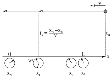
Figure 2: Sketch of the setup. The stimulus moves at constant speed $v$ relative to the oscillator chain. Each time it passes an oscillator the phase is reset to $\psi^{*}$.

The history of phase $\psi_{k}$ can thus be written as

$$\psi_{k}(t)=\left\{{\psi_{k}(0)+\Omega_{k}t\qquad t<t_{k}\atop\psi^{*}+\Omega_{k}(t-t_{k})\quad t\geq t_{k}}\right.$$ (11)

(for all $k=1,\ldots,N)$, where $t_{k}$ is the time when the stimulus passes the oscillator $k$. Substituting this into Eq. (4) we find the following value of the synchronization index:

$$R^{2}(t)={1\over N}+{2\over N^{2}}\left\{S_{kk}(t)+S_{kN}(t)+S_{NN}(t)\right\}$$ (12)

in the time interval $t_{k}\leq t<t_{k+1}$, where we denote

$$S_{kk}(t) = \sum_{i=1}^{k}\sum_{j>i}^{k}\cos\left[\Omega_{i}(t-t_{i})-\Omega_{j}(t-t_{j})\right],$$ (13)

$$S_{kN}(t) = \sum_{i=1}^{k}\sum_{j>k}^{N}\cos\left[\psi^{*}+\Omega_{i}(t-t_{i})-\psi_{j}(0)-\Omega_{j}t\right],$$ (14)

$$S_{NN}(t) = \sum_{i=k+1}^{N}\sum_{j>i}^{N}\cos\left[\psi_{i}(0)+\Omega_{i}t-\psi_{j}(0)-\Omega_{j}t\right]\,.$$ (15)

These expressions depend on the initial phases $\psi_{i}(0)$ and the natural frequencies $\Omega_{i}$. We consider both quantities to be random parameters of the model. To characterize the net effect of observing many realizations, i.e., to evaluate the mean performance of many individuals, we average the synchronization index over both the initial phases (equidistributed) and the natural frequencies (Gaussian). The first average over the phases yields (for $t_{k}\leq t\leq t_{k+1}$)

$$\left<R^{2}(t)\right>={1\over N}+{2\over N^{2}}\sum_{i=1}^{k}\sum_{j>i}^{k}\cos\left[\Omega_{i}(t-t_{i})-\Omega_{j}(t-t_{j})\right]\,.$$ (16)

Note that the value of $\psi^{*}$ is irrelevant for this expression. The second average over the natural frequencies results in

$$\left<\left<R^{2}(t)\right>\right> = {1\over N}+{2\over N^{2}}\sum_{i=1}^{k}\sum_{j>i}^{k}\cos\left[\Omega_{0}(t_{j}-t_{i})\right]$$ (17)

$$\times\;\exp\left\{-{\eta^{2}\Omega_{0}^{2}\over 2}\left[(t-t_{i})^{2}+(t-t_{j})^{2}\right]\right\}.$$

In the following we relate time to the position of the stimulus $x(t)$,

$$t={x_{0}-x(t)\over v}.$$ (18)

We can then derive an expression that reflects how the twice averaged global synchronization index varies as a function of the position of the stimulus over the linear detector chain, namely,

$$\left<\left<R^{2}(x)\right>\right> = {1\over N}+{2\over N^{2}}\sum_{i=1}^{k}\sum_{j>i}^{k}\cos\left[{\Omega_{0}\over v}(x_{i}-x_{j})\right]$$ (19)

$$\times\;\exp\left\{-{\eta^{2}\Omega_{0}^{2}\over 2v^{2}}\left[(x-x_{i})^{2}+(x-x_{j})^{2}\right]\right\},$$

for $x_{k+1}<x\leq x_{k}$. Assuming the oscillators to be distributed along the linear chain in an equidistant manner, i.e., $x_{k}=(N-k)\Delta x$ for $k=1,\ldots,N$ with $\Delta x=L/(N-1)$, we find

$$\left<\left<R^{2}(x)\right>\right> = {1\over N}+{2\over N^{2}}\sum_{i=1}^{k(x)}\sum_{j>i}^{k(x)}\cos\left[(j-i)\kappa\right]$$ (20)

$$\times\;\exp\left\{-{\eta^{2}\kappa^{2}\over 2}g(x,i,j)\right\}\,,$$

where

$$g(x,i,j)=\left[{x\over\Delta x}-(N-i)\right]^{2}+\left[{x\over\Delta x}-(N-j)\right]^{2}$$ (21)

and $k(x)=\min\left\{\mbox{\rm int}[N-{x\over\Delta x}],N\right\}$. The parameter $\kappa$ turns out to be related to the ratio of the travel time between two neighboring oscillators $\Delta T=\Delta x/v$ and the mean rotation period $T_{0}=2\pi/\Omega_{0}$, i.e., $\kappa=2\pi{\Delta T\over T_{0}}$. It is useful to write $\kappa=2\pi m+\delta$, where $m\in N$ and $\delta\in[0,2\pi)$.

Equations (20) and (21) present the central result of our model.

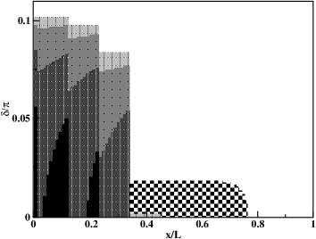
Figure 3: Regions in which prey is detected in the $x$-$\delta$ plane defined by the demand that $\left<\left<R^{2}(x)\right>\right>>R_{\mbox{\tiny\rm th}}^{2}=4/N$. Top panel for $N=100$, $\eta=0$ (black) and $\eta=0.01$ (checkered plotted on top). The bottom panel compares the region for $N=10$ and $\eta=0,0.01,0.02,0.03$ (light to dark gray plotted on top of each other) with $N=100$ and $\eta=0.01$ (checkered). Each time the stimulus passes an detector, $\left<\left<R(x)\right>\right>$ changes discontinously and decays for $\eta>0$.

The detection regions in the $x$-$\delta$ plane, i.e. where $\left<\left<R^{2}(x_{k})\right>\right>$ is larger than the threshold value $R_{\mbox{\tiny\rm th}}^{2}=4/N$, is shown in Fig. 3 for $N=100$ (top) and $N=10$ (bottom). It can be seen that detection works only as long as detuning, quantified by $\delta$, and frequency spread, coded by $\eta$, are not too large. Moreover, we find that the detection region shrinks in the $\delta$ direction, but enlarges in the $x$ direction with increasing $N$, i.e., detection already works when the stimulus has passed only a small number of oscillators. For small $\eta$ and small $\delta$ we can consider the following limiting cases: First let us deal with the case of zero frequency spread, i.e., $\eta=0$. The double sum over cosines can be performed yielding the following expression,

$$\left<\left<R^{2}(x_{k})\right>\right>_{\eta=0}=\frac{N-k+\frac{1-\cos(k\delta)}{1-\cos(\delta)}}{N^{2}},$$ (22)

which we exemplify for $N=100$ in Fig. 4. Depending on the detuning parameter $\delta$, constructive or destructive effects show up.

Figure 4: Variation of the global synchronization index as a function of the stimulus position $x$ in the case of vanishing frequency spread $\eta=0$ for $N=100$. Depending on the detuning parameter $\delta$ constructive or destructive effects of the array or rotors can be observed: $\delta/\pi=0,0.01,0.02,0.03,0.04$ shown as solid, dotted, dashed, long-dashed, dot-dashed lines, respectively. The solid horizontal line marks $R_{\mbox{\tiny\rm th}}^{2}=4/N$

Introducing the frequency spread $\eta>0$ erodes both the constructive and destructive effects. Note that the cycle number $m$ matters if $\eta>0$ whereas it is irrelevant for the case $\eta=0$. In Fig. 5 we exemplify how the detection curve for $N=100$, $m=1$ and a detuning value of $\delta=0.01\pi$ is pushed below the detection threshold by an increasing frequency spread $\eta$.

Figure 5: Spatial variation of the global synchronization index as a function of the stimulus position $x$ in the case of varying frequency spread $\eta$ for slight detuning, i.e., $\delta/\pi=0.01$, and for $m=1$ and $N=100$. An increasing spread erodes the detection mechanism: $\eta=0,0.005,0.01,0.015$ shown as solid, dotted, dashed, long-dashed, respectively. The solid horizontal line marks $R_{\mbox{\tiny\rm th}}^{2}=4/N$

These results indicate that the detection mechanism is rather sensitive with respect to the width of the frequency distribution for a large number $N$ of oscillators. However, we would like to point out, that the biological relevance is not eradicated by this finding, since evolutionary optimization offers an explanation how the confined parameter range might have been realized.

In conclusion, we have presented a simplified but analytically tractable model for signal detection, which works by creating significant coherence in a chain of phase oscillators. This coherence is induced by a strongly localized stimulus that travels at constant speed and resets phases instantaneously. The ability to detect a stimulus rapidly is balanced by the sensitivity to variations in the oscillator frequencies or deviations from the optimal velocity. The variations in the frequencies, however, guarantee a fast desynchronization after the stimulus has passed.

Although our approach concentrates on seemingly crude assumptions, it catches the main features of prey detection. Future experimental studies have to reveal in which direction this model has to be extended to account for given biological applications.

We thank A. Neiman, L. Wilkens and M. Timme for useful discussion. J.F. acknowledges support by the DAAD (NFS-Project No. D/0104610). This work has been supported by the DFG, SFB 555.

References

- [1] L. Wilkens, B. Wettring, E. Wagner, W. Wojtenek, and D. Russell, J. Exp. Biol. 204, 1381 (2001); W. Wojtenek, X. Pei, and L. Wilkens, J. Exp. Biol. 204, 1399 (2001).
- [2] K.-T. Shieh, W. Wilson, M. Winslow, D.W. McBride Jr., and C.D. Hopkins, J. Exp. Biol. 199, 2383 (1996); M.E. Nelson and M.A. MacIver, J. Exp. Biol. 202, 1195 (1999); G. von der Emde, J. Exp. Biol. 202, 1205 (1999).
- [3] A. Neiman and D.F. Russell, Phys. Rev. Lett. 86 3443 (2001); A. Neiman, X. Pei, D. Russell, W. Wojtenek, L. Wilkens, F. Moss, H.A. Braun, M.T. Huber, and K. Voigt, Phys. Rev. Lett. 82, 660 (1999); R.W. Turner and L. Maler, J. Exp. Biol. 202, 1255 (1999).
- [4] A. Pikovsky, M. Rosenblum, and J. Kurths, Synchronization – A Universal Concept in Nonlinear Sciences, (Cambridge University Press, Cambridge, 2001).
- [5] M. Fisz Probability Theory and Mathematical Statistics, (John Wiley & Sons, 1963)
- [6] P. Tass, Phase Resetting in Medicine and Biology, (Springer, Berlin, 2001); A.T. Winfree, J. Theor. Biol. 28, 327 (1970).