Resonant laser excitation of molecular wires

Abstract

We investigate the influence of external laser excitations on the average current through bridged molecules. For the computation of the current, we use a numerically very efficient formalism that is based on the Floquet solutions of the time-dependent molecule Hamiltonian. It is found that the current as a function of the laser frequency exhibits characteristic peaks originating from resonant excitations of electrons to bridge levels which are unoccupied in the absence of the radiation. The electrical current through the molecule can exhibit a drastic enhancement by several orders of magnitude.

I Introduction

In a seminal work Aviram1974a , Aviram and Ratner proposed almost thirty years ago to build elements of electronic circuits — in their case a rectifier — with single molecules. In the present days their vision starts to become reality and the experimental and theoretical study of such systems enjoys a vivid activity Joachim2000a ; Nitzan2001a ; Hanggi2002a . Recent experimental progress has enabled reproducible measurements Cui2001a ; Reichert2002a of weak tunneling currents through molecules which are coupled by chemisorbed thiol groups to the gold surface of external leads. A necessary ingredient for future technological applications will be the possibility to control the tunneling current through the molecule.

Typical energy scales in molecules are in the optical and the infrared regime, where basically all of the today’s lasers operate. Hence, lasers represent a natural possibility to control atoms or molecules and also currents through them. It is for example possible to induce by the laser field an oscillating current in the molecule which under certain asymmetry conditions is rectified by the molecule resulting in a directed electron transport even in the absence of any applied voltage Lehmann2002b ; Lehmann2002d . Another theoretically predicted effect is the current suppression by the laser field Lehmann2002c which offers the possibility to control and switch the electron transport by light. Since the considered frequencies lie below typical plasma frequencies of metals, the laser light will be reflected at the metal surface, i.e. it does not penetrate the leads. Consequently, we do not expect major changes of the leads’ bulk properties — in particular each lead remains close to equilibrium. Thus, to a good approximation, it is sufficient to consider the influence of the driving solely in the molecule Hamiltonian. In addition, the energy of infrared light quanta is by far smaller than the work function of a common metal, which is of the order of $5\,\mathrm{eV}$. This prevents the generation of a photo current, which otherwise would dominate the effects discussed below.

Recent theoretical descriptions of the molecular conductivity in non-driven situations are based on a scattering approach Mujica1994a ; Datta1995a , or assume that the underlying transport mechanism is an electron transfer reaction from the donor to the acceptor site and that the conductivity can be derived from the corresponding reaction rates Nitzan2001a . It has been demonstrated that both approaches yield essentially identical results in a large parameter regime Nitzan2001b . Within a high-temperature limit, the electron transport on the wire can be described by inelastic hopping events Petrov2001a ; Lehmann2002a .

Atoms and molecules in strong oscillating fields have been widely studied within a Floquet formalism Manakov1986a ; Grifoni1998a . This suggests utilizing the tools that have been acquired in that area, thus, developing a transport formalism that combines Floquet theory for a driven molecule with the many-particle description of transport through a system that is coupled to ideal leads Lehmann2002b ; Lehmann2002c ; Lehmann2002d . Such an approach is devised much in the spirit of the Floquet-Markov theory Blumel1989a ; Kohler1997a for driven dissipative quantum systems.

II Floquet treatment of the electron transport

The entire system of the wire in the laser-field, the leads, and the molecule-lead coupling as sketched in Figure 1 is described by the Hamiltonian

$$H(t)=H_{\text{wire}}(t)+H_{\text{leads}}+H_{\text{wire-leads}}\,.$$ (1)

The wire is modeled by $N$ atomic orbitals $|n\rangle$, $n=1,\ldots,N$, which are in a tight-binding description coupled by hopping matrix elements. Then, the corresponding Hamiltonian for the electrons on the wire reads in a second quantized form

$$H_{\text{wire}}(t)=\sum_{n,n^{\prime}}H_{nn^{\prime}}(t)\,c_{n}^{\dagger}c_{n^{\prime}},$$ (2)

where the fermionic operators $c_{n}$, $c_{n}^{\dagger}$ annihilate, respectively create, an electron in the atomic orbital $|n\rangle$ and obey the anti-commutation relation $[c_{n},c_{n^{\prime}}^{\dagger}]_{+}=\delta_{n,n^{\prime}}$. The influence of the laser field is given by a periodic time-dependence of the on-site energies yielding a single particle Hamiltonian of the structure $H_{nn^{\prime}}(t)=H_{nn^{\prime}}(t+\mathcal{T})$, where $\mathcal{T}=2\pi/\Omega$ is determined by the frequency $\Omega$ of the laser field.

The orbitals $|1\rangle$ and $|N\rangle$ at the left and the right end of the molecule, that we shall term donor and acceptor, respectively, are coupled to ideal leads (cf. Fig. 1) by the tunneling Hamiltonians

$$H_{\text{wire-leads}}=\sum_{q}(V_{qL}\,c_{qL}^{\dagger}c_{1}+V_{qR}\,c_{qR}^{\dagger}c_{N})+\mathrm{H.c.}$$ (3)

The operator $c_{qL}$ ($c_{qR}$) annihilates an electron in state $Lq$ ($Rq$) on the left (right) lead. The leads are modeled as non-interacting electrons with the Hamiltonian

$$H_{\rm leads}=\sum_{q}(\epsilon_{qL}\,c_{qL}^{\dagger}c_{qL}+\epsilon_{qR}\,c_{qR}^{\dagger}c_{qR}),$$ (4)

where $\epsilon_{qL}$ is the single particle energy of the state $qL$ and correspondingly for the right lead. As discussed above, the leads can be described by a grand-canonical ensemble of electrons, i.e. by a density matrix

$$\varrho_{\mathrm{leads,eq}}\propto\exp\left[{-(H_{\mathrm{leads}}-\mu_{L}N_{L}-\mu_{R}N_{R})/k_{B}T}\right],$$ (5)

where $\mu_{L/R}$ are the electro-chemical potentials and $N_{L/R}=\sum_{q}c^{\dagger}_{qL/R}c_{qL/R}$ the electron numbers in the left/right lead. As a consequence, the only non-trivial expectation values of lead operators read

$$\langle c_{qL}^{\dagger}c_{qL}\rangle=f(\epsilon_{qL}-\mu_{L}).$$ (6)

Here, $f(x)=(1+e^{x/k_{B}T})^{-1}$ denotes the Fermi function.

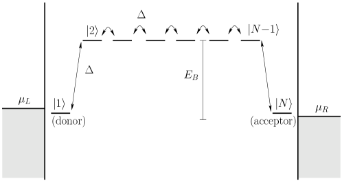
Figure 1: Level structure of a molecular wire with $N=8$ atomic sites which are attached to two leads.

II.1 Perturbation theory

While the leads and the wire, including the driving, will be treated exactly, we take the wire-lead Hamiltonian as a perturbation into account. Starting from the Liouville-von Neumann equation $i\hbar\dot{\varrho}(t)=[H(t),\varrho(t)]$ together with the factorizing initial condition $\varrho(t_{0})=\varrho_{\mathrm{wire}}(t_{0})\otimes\varrho_{\mathrm{leads,eq}}$, we derive by standard techniques an approximate equation of motion for the total density operator $\varrho(t)$. This is most conveniently achieved in the interaction picture with respect to the uncoupled dynamics where the Liouville-von Neumann equation reads

$$i\hbar\frac{d}{dt}\tilde{\varrho}(t,t_{0})=[\widetilde{H}_{\mathrm{wire-leads}}(t,t_{0}),\tilde{\varrho}(t,t_{0})].$$ (7)

The tilde denotes the corresponding interaction picture operators, $\widetilde{X}(t,t^{\prime})=U_{0}^{\dagger}(t,t^{\prime})\,X(t)\,U_{0}(t,t^{\prime})$ where the propagator of the wire and the lead in the absence of the lead-wire coupling is given by the time-ordered product

$$U_{0}(t,t^{\prime})={\stackrel{{\scriptstyle\leftarrow}}{{\textstyle T}}}\exp\left(-\frac{i}{\hbar}\int_{t^{\prime}}^{t}dt^{\prime\prime}\,[H_{\mathrm{wire}}(t^{\prime\prime})+H_{\mathrm{leads}}]\right).$$ (8)

Equation (7) is equivalent to the following integral equation

$$\tilde{\varrho}(t,t_{0})=\tilde{\varrho}(t_{0},t_{0})-\frac{i}{\hbar}\int_{t_{0}}^{t}dt^{\prime}[\widetilde{H}_{\mathrm{wire-leads}}(t^{\prime},t_{0}),\tilde{\varrho}(t^{\prime},t_{0})].$$ (9)

We reinsert this expression into the differential equation (7) and use that to zeroth order in the molecule-lead coupling the interaction-picture density operator does not change with time, $\tilde{\varrho}(t-\tau,t_{0})\approx\tilde{\varrho}(t,t_{0})$. A transformation back to the Schrödinger picture results in the following approximate equation of motion for the total density operator Lehmann2002b ; Lehmann2002d

$$\begin{split}\dot{\varrho}(t)=&-\frac{i}{\hbar}[H_{\rm wire}(t)+H_{\rm leads},\varrho(t)]-\frac{1}{\hbar^{2}}\int\limits_{0}^{\infty}\!\!d\tau[H_{\mathrm{wire-leads}},[\widetilde{H}_{\mathrm{wire-leads}}(t-\tau,t),\varrho(t)]]\\ &-\frac{i}{\hbar}[H_{\mathrm{wire-leads}},U_{0}(t,t_{0})\varrho(t_{0})U_{0}^{\dagger}(t,t_{0})].\end{split}$$ (10)

Since we only consider asymptotic times $t-t_{0}\to\infty$, we have set the upper limit in the integral to infinity. The third term in Eq. (10) stems from the initial condition at $t_{0}$ in the integrated form (9) of the Liouville-von Neumann equation. For the chosen factorizing initial condition, it will not contribute to the expectation values calculated below.

The net (incoming minus outgoing) current through the left contact is given by the negative time derivative of the electron number in the left lead, multiplied by the electron charge $-e$, i.e.

$$I_{L}(t)=e\mathop{\rm tr}[\dot{\varrho}(t)N_{L}].$$ (11)

We insert $\dot{\varrho}(t)$ from Eq. (10) and obtain an expression that depends on the density of states in the leads times their coupling strength to the connected sites. At this stage it is convenient to introduce the spectral density of the lead-wire coupling

$$\Gamma_{L/R}(\epsilon)=\frac{2\pi}{\hbar}\sum_{q}|V_{qL/R}|^{2}\delta(\epsilon-\epsilon_{qL/R}),$$ (12)

which fully describes the leads’ influence. If the lead states are dense, $\Gamma_{L/R}(\epsilon)$ becomes a continuous function. Because we are mainly interested in the behavior of the molecule and not in the details of the lead-wire coupling, we assume that the conduction band width of the leads is much larger than all remaining relevant energy scales. Consequently, we approximate in the so-called wide-band limit the functions $\Gamma_{L/R}(\epsilon)$ by the constant values $\Gamma_{L/R}$. After some algebra, we find for the time-dependent net electrical current through the left contact the expression

$$I_{L}(t)=\frac{e\Gamma_{L}}{\pi\hbar}\mathop{\rm Re}\int\limits_{0}^{\infty}\!d\tau\!\int\!d\epsilon\,e^{i\epsilon\tau/\hbar}\Big{\{}\big{\langle}\tilde{c}_{1}^{\dagger}(t-\tau,t)\,c_{1}\big{\rangle}-[c_{1},\tilde{c}_{1}^{\dagger}(t-\tau,t)]_{+}f(\epsilon-\mu_{L})\Big{\}},$$ (13)

and correspondingly for the current through the contact on the right-hand side. Here, we made the assumption, that the leads are at all times well described by the density operator (5). Note that the anti-commutator $[c_{1},\tilde{c}_{1}^{\dagger}(t-\tau,t)]_{+}$ is in fact a c-number. Like the expectation value $\langle c_{1}^{\dagger}(t-\tau,t)\,c_{1}\rangle$ it depends on the dynamics of the isolated wire and is influenced by the external driving. The first contribution of the $\epsilon$-integral in Eq. (13) is readily evaluated to yield an expression proportional to $\delta(\tau)$. Thus, this term becomes local in time and reads $e\Gamma_{L}\big{\langle}c_{1}^{\dagger}c_{1}\big{\rangle}$.

II.2 Floquet decomposition

Let us next focus on the single-particle dynamics of the driven molecule decoupled from the leads. Since its Hamiltonian is periodic in time, $H_{nn^{\prime}}(t)=H_{nn^{\prime}}(t+\mathcal{T})$, we can solve the corresponding time-dependent Schrödinger equation within a Floquet approach. This means that we make use of the fact that there exists a complete set of solutions of the form Shirley1965a ; Sambe1973a ; Fainshtein1978a ; Hanggi1998a ; Grifoni1998a

$$|\Psi_{\alpha}(t)\rangle=e^{-i\epsilon_{\alpha}t/\hbar}|\Phi_{\alpha}(t)\rangle,\ |\Phi_{\alpha}(t)\rangle=|\Phi_{\alpha}(t+\mathcal{T})\rangle$$ (14)

with the quasi-energies $\epsilon_{\alpha}$. Since the so-called Floquet modes $|\Phi_{\alpha}(t)\rangle$ obey the time-periodicity of the driving field, they can be decomposed into the Fourier series

$$|\Phi_{\alpha}(t)\rangle=\sum_{k}e^{-ik\Omega t}|\Phi_{\alpha,k}\rangle.$$ (15)

This implies that the quasienergies $\epsilon_{\alpha}$ come in classes,

$$\epsilon_{\alpha,k}=\epsilon_{\alpha}+k\hbar\Omega,\quad k=0,\pm 1,\pm 2,\ldots,$$ (16)

of which all members represent the same solution of the Schrödinger equation. Therefore, the quasienergy spectrum can be reduced to a single “Brillouin zone” $-\hbar\Omega/2\leq\epsilon<\hbar\Omega/2$. In turn, all physical quantities that are computed within a Floquet formalism are independent of the choice of a specific class member. Thus, a consistent description must obey the so-called class invariance, i.e. it must be invariant under the substitution of one or several Floquet states by equivalent ones,

$$\epsilon_{\alpha},\,|\Phi_{\alpha}(t)\rangle\longrightarrow\epsilon_{\alpha}+k_{\alpha}\hbar\Omega,\,e^{ik_{\alpha}\Omega t}|\Phi_{\alpha}(t)\rangle,$$ (17)

where $k_{1},\dots,k_{N}$ are integers. In the Fourier decomposition (15), the prefactor $\exp({ik_{\alpha}\Omega t})$ corresponds to a shift of the side band index so that the class invariance can be expressed equivalently as

$$\epsilon_{\alpha},\,|\Phi_{\alpha,k}\rangle\longrightarrow\epsilon_{\alpha}+k_{\alpha}\hbar\Omega,\,|\Phi_{\alpha,k+k_{\alpha}}\rangle.$$ (18)

Floquet states and quasienergies can be obtained from the quasienergy equation Shirley1965a ; Sambe1973a ; Fainshtein1978a ; Manakov1986a ; Hanggi1998a ; Grifoni1998a

$$\Big{(}\sum_{n,n^{\prime}}|n\rangle H_{nn^{\prime}}(t)\langle n^{\prime}|-i\hbar\frac{d}{dt}\Big{)}|\Phi_{\alpha}(t)\rangle=\epsilon_{\alpha}|\Phi_{\alpha}(t)\rangle.$$ (19)

A wealth of methods for the solution of this eigenvalue problem can be found in the literature. For an overview, we refer the reader to the reviews in Refs.  Hanggi1998a, ; Grifoni1998a, , and the references therein.

As the equivalent of the one-particle Floquet states $|\Phi_{\alpha}(t)\rangle$, we define a Floquet picture for the fermionic creation and annihilation operators $c_{n}^{\dagger}$, $c_{n}$, by the time-dependent transformation

$$c_{\alpha}(t)=\sum_{n}\langle\Phi_{\alpha}(t)|n\rangle\,c_{n}.$$ (20)

The inverse transformation

$$c_{n}=\sum_{\alpha}\langle n|\Phi_{\alpha}(t)\rangle\,c_{\alpha}(t)$$ (21)

follows from the mutual orthogonality and the completeness of the Floquet states at equal times Hanggi1998a ; Grifoni1998a . Note that the right-hand side of Eq. (21) becomes $t$-independent after the summation. The operators $c_{\alpha}(t)$ are constructed in such a way that the time-dependences of the interaction picture operators $\tilde{c}_{\alpha}(t-\tau,t)$ separate, which will turn out to be crucial for the further analysis. Indeed, one can easily verify the relation

$$\begin{split}\tilde{c}_{\alpha}(t-\tau,t)&=U_{0}^{\dagger}(t-\tau,t)\,c_{\alpha}(t-\tau)\,U_{0}(t-\tau,t)\\ &=e^{i\epsilon_{\alpha}\tau/\hbar}c_{\alpha}(t)\end{split}$$ (22)

by differentiating the definition in the first line with respect to $\tau$ and using that $|\Phi_{\alpha}(t)\rangle$ is a solution of the eigenvalue equation (19). The fact that the initial condition $\tilde{c}_{\alpha}(t,t)=c_{\alpha}(t)$ is fulfilled completes the proof. The corresponding expression for the interaction picture operator in the on-site basis, $\tilde{c}_{n}(t-\tau,t)$, can be derived with help of Eq. (21) at time $t-\tau$ together with (22) to read

$$\tilde{c}_{n}(t-\tau,t) =\sum_{\alpha}\langle n|\Phi_{\alpha}(t-\tau)\rangle e^{i\epsilon_{\alpha}\tau/\hbar}c_{\alpha}(t)$$ (23)

$$=\sum_{\alpha k}e^{i(\epsilon_{\alpha}/\hbar+k\Omega)\tau}e^{-ik\Omega t}\langle n|\Phi_{\alpha,k}\rangle c_{\alpha}(t).$$ (24)

Equations (22), (24), consequently allow to express the interaction picture operator $\tilde{c}_{1}^{\dagger}(t-\tau,t)$ appearing in the current formula (13) via $c_{\alpha}(t)$, dressed by exponential prefactors.

This spectral decomposition allows one to carry out the time and energy integrals in the expression (13) for the net current entering the wire from the left lead. Thus, we obtain

$$I_{L}(t)=\sum_{k}e^{-ik\Omega t}I_{L}^{k},$$ (25)

with the corresponding Fourier components

$$\begin{split}I_{L}^{k}={}&e\Gamma_{L}\bigg{[}\sum_{\alpha\beta k^{\prime}k^{\prime\prime}}\langle\Phi_{\alpha,k^{\prime}+k^{\prime\prime}}|1\rangle\langle 1|\Phi_{\beta,k+k^{\prime\prime}}\rangle R_{\alpha\beta,k^{\prime}}\\ &\qquad-\frac{1}{2}\sum_{\alpha k^{\prime}}\Big{(}\langle\Phi_{\alpha,k^{\prime}}|1\rangle\langle 1|\Phi_{\alpha,k+k^{\prime}}\rangle+\langle\Phi_{\alpha,k^{\prime}-k}|1\rangle\langle 1|\Phi_{\alpha,k^{\prime}}\rangle\Big{)}f(\epsilon_{\alpha,k^{\prime}}-\mu_{L})\bigg{]}.\end{split}$$ (26)

Here, we have introduced the expectation values

$$R_{\alpha\beta}(t) =\langle c_{\alpha}^{\dagger}(t)c_{\beta}(t)\rangle=R_{\beta\alpha}^{*}(t)$$ (27)

$$=\sum_{k}e^{-ik\Omega t}R_{\alpha\beta,k}.$$ (28)

The Fourier decomposition in the last line is possible because all $R_{\alpha\beta}(t)$ are expectation values of a linear, dissipative, periodically driven system and therefore share in the long-time limit the time-periodicity of the driving field. In the subspace of a single electron, $R_{\alpha\beta}$ reduces to the density matrix in the basis of the Floquet states which has been used to describe dissipative driven quantum systems in Refs.  Blumel1991a, ; Dittrich1993a, ; Kohler1997a, ; Kohler1998a, ; Grifoni1998a, ; Hanggi2000a, .

The next step towards the stationary current is to find the Fourier coefficients $R_{\alpha\beta,k}$ at asymptotic times. To this end, we derive from the equation of motion (10) a master equation for $R_{\alpha\beta}(t)$. Since all coefficients of this master equation, as well as its asymptotic solution, are $\mathcal{T}$-periodic, we can split it into its Fourier components. Finally, we obtain for the $R_{\alpha\beta,k}$ the inhomogeneous set of equations

$${\frac{i}{\hbar}(\epsilon_{\alpha}-\epsilon_{\beta}+k\hbar\Omega)R_{\alpha\beta,k}}= \frac{\Gamma_{L}}{2}\sum_{k^{\prime}}\Big{(}\sum_{\beta^{\prime}k^{\prime\prime}}\langle\Phi_{\beta,k^{\prime}+k^{\prime\prime}}|1\rangle\langle 1|\Phi_{\beta^{\prime},k+k^{\prime\prime}}\rangle R_{\alpha\beta^{\prime},k^{\prime}}$$ (29)

$$\hskip 25.83325pt+\sum_{\alpha^{\prime}k^{\prime\prime}}\langle\Phi_{\alpha^{\prime},k^{\prime}+k^{\prime\prime}}|1\rangle\langle 1|\Phi_{\alpha,k+k^{\prime\prime}}\rangle R_{\alpha^{\prime}\beta,k^{\prime}}$$

$$\hskip 25.83325pt-\langle\Phi_{\beta,k^{\prime}-k}|1\rangle\langle 1|\Phi_{\alpha,k^{\prime}}\rangle f(\epsilon_{\alpha,k^{\prime}}-\mu_{L})$$

$$\hskip 25.83325pt-\langle\Phi_{\beta,k^{\prime}}|1\rangle\langle 1|\Phi_{\alpha,k^{\prime}+k}\rangle f(\epsilon_{\beta,k^{\prime}}-\mu_{L})\Big{)}$$

$${}+\text{same terms with the replacement}$$

$$\hskip 8.61108pt{}{\big{\{}\Gamma_{L},\mu_{L},|1\rangle\langle 1|\big{\}}\rightarrow\big{\{}\Gamma_{R},\mu_{R},|N\rangle\langle N|\big{\}}}.$$

For a consistent Floquet description, the current formula together with the master equation must obey class invariance. Indeed, the simultaneous transformation with (18) of both the master equation (29) and the current formula (26) amounts to a mere shift of summation indices and, thus, leaves the current as a physical quantity unchanged.

For the typical parameter values used below, a large number of sidebands contributes significantly to the Fourier decomposition of the Floquet modes $|\Phi_{\alpha}(t)\rangle$. Numerical convergence for the solution of the master equation (29), however, is already obtained by just using a few sidebands for the decomposition of $R_{\alpha\beta}(t)$. This keeps the numerical effort relatively small and justifies a posteriori the use of the Floquet representation (21). Yet we are able to treat the problem beyond the rotating-wave-approximation.

II.3 Time-averaged current through the molecular wire

Equation (25) implies that the current $I_{L}(t)$ obeys the time-periodicity of the driving field. Since we consider here excitations by a laser field, the corresponding driving frequency lies in the optical or infrared spectral range. In an experiment one will thus only be able to measure the time-average of the current. For the net current entering through the left contact it is given by

$$\begin{split}\bar{I}_{L}=I^{0}_{L}=e\Gamma_{L}\sum_{\alpha k}\Big{[}&\sum_{\beta k^{\prime}}\langle\Phi_{\alpha,k^{\prime}+k}|1\rangle\langle 1|\Phi_{\beta,k^{\prime}}\rangle R_{\alpha\beta,k}-\langle\Phi_{\alpha,k}|1\rangle\langle 1|\Phi_{\alpha,k}\rangle f(\epsilon_{\alpha,k}-\mu_{L})\Big{]}.\end{split}$$ (30)

By replacing $\{|1\rangle,L\}\to\{|N\rangle,R\}$, one obtains for the current which enters from the right, $I_{R}(t)$, and the corresponding Fourier coefficients and time averages.

Total charge conservation of the original wire-lead Hamiltonian (1) of course requires that the charge on the wire can only change by current flow, amounting to the continuity equation $\dot{Q}_{\mathrm{wire}}(t)=I_{L}(t)+I_{R}(t)$. Since asymptotically, the charge on the wire obeys at most the periodic time-dependence of the driving field, the time-average of $\dot{Q}_{\mathrm{wire}}(t)$ must vanish in the long-time limit. From the continuity equation one then finds that $\bar{I}_{L}+\bar{I}_{R}=0$, and we can introduce the time-averaged current

$$\bar{I}=\bar{I}_{L}=-\bar{I}_{R}.$$ (31)

This continuity equation can be obtained directly from the average current formula (30) together with the master equation (29), as has been explicitly shown in Ref.  Lehmann2002d, .

III Laser-enhanced current

III.1 Bridged molecular wire

As a working model we consider a molecule consisting of a donor and an acceptor site and $N-2$ sites in between (cf. Fig. 1). Each of the $N$ sites is coupled to its nearest neighbors by a hopping matrix elements $\Delta$. The laser field renders each level oscillating in time with a position-dependent amplitude. Thus, the corresponding time-dependent wire Hamiltonian reads

$$\begin{split}H_{nn^{\prime}}(t)=&-\Delta(\delta_{n,n^{\prime}+1}+\delta_{n+1,n^{\prime}})+\left[E_{n}-A\,x_{n}\cos(\Omega t)\right]\delta_{nn^{\prime}},\end{split}$$ (32)

where $x_{n}=(N+1-2n)/2$ is the scaled position of site $|n\rangle$. The energy $a(t)$ equals the electron charge multiplied by the electrical field amplitude of the laser and the distance between two neighboring sites. The energies of the donor and the acceptor orbitals are assumed to be at the level of the chemical potentials of the attached leads, $E_{1}=E_{N}=\mu_{L}=\mu_{R}$. The bridge levels $E_{n}$, $n=2,\dots,N-1$, lie $E_{B}\gg\Delta$ above the chemical potential, as sketched in Figure 1.

In all numerical studies, we will use a symmetric coupling, $\Gamma_{L}=\Gamma_{R}=\Gamma$. The hopping matrix element $\Delta$ serves as the energy unit; in a realistic wire molecule, $\Delta$ is of the order $0.1\,{\rm eV}$. Thus, our chosen wire-lead hopping rate $\Gamma=0.1\Delta/\hbar$ yields $e\Gamma=2.56\times 10^{-5}$ Ampère and $\Omega\approx 10\Delta/\hbar$ corresponds to a laser frequency in the near infrared. For a typical distance of $5$Å between two neighboring sites, a driving amplitude $A=\Delta$ is equivalent to an electrical field strength of $2\times 10^{6}\,\mathrm{V/cm}$.

III.2 Average current at resonant excitations

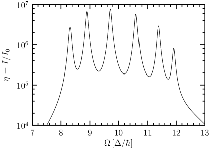
Figure 2: Amplification of the time-averaged current through the wire sketched in Figure 1 with $E_{B}=10\Delta$. The scaled amplitude is $A=0.1\Delta$; the applied voltage $\mu_{L}-\mu_{R}=5\Delta/e$. The other parameters read $\Gamma=\Gamma_{L}=\Gamma_{R}=0.1\Delta/\hbar$, $k_{B}T=0.25\Delta$.

Figure 3: Average current $\bar{I}$ as a function of the the driving frequency $\Omega$ for various driving amplitudes $A$ and coupling strength $\Gamma=\Gamma_{L}=\Gamma_{R}$. All the other parameters are as in Fig. 2.

Figure 4: Average current $\bar{I}$ as a function of the the driving frequency $\Omega$ for various wire length $N$. All the other parameters are as in Fig. 2.

Let us first discuss the static problem in the absence of the field, i.e. for $A=0$. In the present case where the coupling between two neighboring sites is much weaker than the bridge energy, $\Delta\ll E_{B}$, one finds two types of eigenstates: One forms a doublet whose states are approximately given by $(|1\rangle\pm|N\rangle)/\sqrt{2}$. Its splitting can be estimated in a perturbational approach Ratner1990a and is approximately given by $2\Delta(\Delta/E_{B})^{N-2}$. A second group of states is located on the bridge. It consists of $N-2$ levels with energies in the range $[E_{B}-2\Delta,E_{B}+2\Delta]$. In the absence of the driving field, these bridge states mediate the super-exchange between the donor and the acceptor. This yields an exponentially decaying length dependence of the conductance Mujica1994a ; Nitzan2001a .

This behavior changes significantly when a driving field with a frequency $\Omega\approx E_{B}/\hbar$ is switched on. Then the resonant bridge levels merge with the donor and the acceptor state to form a Floquet state. This opens a direct channel for the transport resulting in an enhancement of the electron current as depicted in Figure 2 where we plot the current amplification, defined as the ratio of the time-averaged current to the current in the absence of the laser, $\eta=\bar{I}/I_{0}$: In a wire with $N=8$ sites, one finds peaks in the current when the driving frequency matches the energy difference between the donor/acceptor doublet and one of the $N-2=6$ bridge levels. The applied voltage is always chosen so small that the bridge levels lie below the chemical potentials of the leads. The amplification, can assume many orders of magnitude, cf. Figure 2. Generally, the response of a system to a weak resonant driving scales with the damping and the driving amplitude. Figure 3 demonstrates this behavior for the peaks of the electrical current. The peak heights at the maxima of the time-averaged current are found proportional to $A^{2}/\Gamma$. A further scaling behavior is found for the current peaks as a function of the wire length: The average current no longer exhibits the exponentially decaying length dependence that has been found for bridged super-exchange. By contrast, it emerges proportional to $1/(N-1)$. This can be appreciated in Figure 4 where the scale of the abscissa is chosen proportional to $N-1$ such that it suggests a common envelope function. Put differently, the current is essentially inversely proportional to the length as in the case of Ohmic conductance.

In summary, we find current peaks whose height $\bar{I}_{\mathrm{peak}}$ scales according to

$$\bar{I}_{\mathrm{peak}}\propto\frac{A^{2}}{(N-1)\Gamma}.$$ (33)

Thus, the current is especially for long wires much larger than the corresponding current in the absence of the driving.

IV Conclusions

We have presented a detailed derivation of the Floquet transport formalism which has been applied in Refs.  Lehmann2002b, ; Lehmann2002c, ; Lehmann2002d, . The analysis of a bridged molecular wire revealed that resonant excitations from the levels that connect the molecule to the external leads to bridge levels yield peaks in the current as a function of the driving frequency. In a regime with weak driving and weak electron-lead coupling, $\Delta\gg\Gamma,A$, the peak heights scale with the coupling strength, the driving amplitude, and the wire length. The laser irradiation induces a large current enhancement of several orders of magnitude. The observation of these resonances could serve as an experimental starting point for the more challenging attempt of measuring quantum ratchet effects Lehmann2002b ; Lehmann2002d or current switching by laser fields Lehmann2002c .

V acknowledgement

This work has been supported by SFB 486 and by the Volkswagen-Stiftung under grant No. I/77 217. One of us (S.C.) has been supported by a European Community Marie Curie Fellowship.

References

- (1) A. Aviram and M. A. Ratner, Chem. Phys. Lett. 29, 277 (1974).
- (2) C. Joachim, J. K. Gimzewski, and A. Aviram, Nature 408, 541 (2000).
- (3) A. Nitzan, Annu. Rev. Phys. Chem. 52, 681 (2001).
- (4) P. Hänggi, M. Ratner, and S. Yaliraki, Special Issue: Processes in Molecular Wires, Chem. Phys. 281, pp. 111-502 (2002).
- (5) X. D. Cui et al., Science 294, 571 (2001).
- (6) J. Reichert, R. Ochs, D. Beckmann, H. B. Weber, M. Mayor, and H. v. Löhneysen, Phys. Rev. Lett. 88, 176804 (2002).
- (7) J. Lehmann, S. Kohler, P. Hänggi, and A. Nitzan, Phys. Rev. Lett. 88, 228305 (2002).
- (8) J. Lehmann, S. Kohler, P. Hänggi, and A. Nitzan, cond-mat/ 0208404 (2002).
- (9) J. Lehmann, S. Camalet, S. Kohler, and P. Hänggi, physics/ 0205060 (2002).
- (10) V. Mujica, M. Kemp, and M. A. Ratner, J. Chem. Phys. 101, 6849 (1994).
- (11) S. Datta, Electronic Transport in Mesoscopic Systems (Cambridge University Press, Cambridge, 1995).
- (12) A. Nitzan, J. Phys. Chem. A 105, 2677 (2001).
- (13) E. G. Petrov and P. Hänggi, Phys. Rev. Lett. 86, 2862 (2001).
- (14) J. Lehmann, G.-L. Ingold, and P. Hänggi, Chem. Phys. 281, 199 (2002).
- (15) N. L. Manakov, V. D. Ovsiannikov, and L. P. Rapoport, Phys. Rep. 141, 319 (1986).
- (16) M. Grifoni and P. Hänggi, Phys. Rep. 304, 229 (1998).
- (17) R. Blümel, R. Graham, L. Sirko, U. Smilansky, H. Walther, and K. Yamada, Phys. Rev. Lett. 62, 341 (1989).
- (18) S. Kohler, T. Dittrich, and P. Hänggi, Phys. Rev. E 55, 300 (1997).
- (19) J. H. Shirley, Phys. Rev. 138, B979 (1965).
- (20) H. Sambe, Phys. Rev. A 7, 2203 (1973).
- (21) A. G. Fainshtein, N. L. Manakov, and L. P. Rapoport, J. Phys. B 11, 2561 (1978).
- (22) P. Hänggi, in Quantum Transport and Dissipation (Wiley-VCH, Weinheim, 1998).
- (23) R. Blümel, A. Buchleitner, R. Graham, L. Sirko, U. Smilansky, and H. Walter, Phys. Rev. A 44, 4521 (1991).
- (24) T. Dittrich, B. Oelschlägel, and P. Hänggi, Europhys. Lett. 22, 5 (1993).
- (25) S. Kohler, R. Utermann, P. Hänggi, and T. Dittrich, Phys. Rev. E 58, 7219 (1998).
- (26) P. Hänggi, S. Kohler, and T. Dittrich, in Statistical and Dynamical Aspects of Mesoscopic Systems, Vol. 547 of Lecture Notes in Physics, edited by D. Reguera, G. Platero, L. L. Bonilla, and J. M. Rubí (Springer, Berlin, 2000), pp. 125–157.
- (27) M. A. Ratner, J. Phys. Chem. 94, 4877 (1990).