Computational studies of light acceptance and propagation in straight and curved optical fibres

Abstract

A Monte Carlo simulation has been performed to track light rays in cylindrical fibres by ray optics. The trapping efficiencies for skew and meridional rays in active fibres and distributions of characteristic quantities for all trapped light rays have been calculated. The simulation provides new results for curved fibres, where the analytical expressions are too complex to be solved. The light losses due to sharp bending of fibres are presented as a function of the ratio of curvature to fibre radius and bending angle. It is shown that a radius of curvature to fibre radius ratio of greater than 65 results in a loss of less than 10% with the loss occuring in the initial stage of the bend (at bending angles $\Phi\sim\pi/8$ rad).

1 Introduction

Active optical fibres are becoming more and more important in the field of detection and measurement of ionising radiation and particles. Light is generated inside the fibre either through interaction with the incident radiation (scintillating fibres) or through absorption of primary light (wavelength-shifting fibres). Plastic fibres with large core diameters, i.e. where the wavelength of the light being transmitted is much smaller than the fibre diameter, are commercially available and readily fabricated, have good timing properties and allow a multitude of different geometrical designs. The low costs of plastic materials make it possible for many experiments to use such fibres in large quantities, particularly in highly segmented tracking detectors and sampling calorimeters (see reference [1] for a review of plastic fibres in high energy physics). Although for many years fibres have been the subject of extensive studies, only fragmentary calculations of trapping efficiencies and light losses in curved fibres have been performed for multi-mode fibres. We have therefore performed a full simulation of photons propagating in simple circularly curved fibres in order to quantify the losses caused by the bending and to establish the dependence of these losses on the angle of the bend. We have also briefly investigated the time dispersion in fibres. For our calculations the most common type of fibre in particle physics is assumed. This standard fibre is specified by a polystyrene core of refractive index $n_{\it core}=$ 1.6 and a thin polymethylmethacrylate (PMMA) cladding of refractive index $n_{\it clad}=$ 1.49, where the indices are given at a wavelength of 590 nm. Another common cladding material is fluorinated polymethacrylate which has a slightly lower index of reflection of $n_{\it clad}=1.42$. Typical diameters are in the range of 0.5 – 1.5 mm.

The treatment of small diameter optical fibres involves electromagnetic theory applied to dielectric waveguides, which was first achieved by Snitzer [2] and Kapany [3]. Although this approach provides insight into the phenomenon of total internal reflection and eventually leads to results for the field distributions and electromagnetic radiation for curved fibres, it is advantageous to use ray optics for applications to large diameter fibres where the waveguide analysis is an unnecessary complication. In ray optics a light ray may be characterised by its path along the fibre. The path of a meridional ray is confined to a single plane, all other modes of propagation are known as skew rays. In general, the projection of a meridional ray on a plane perpendicular to the fibre axis is a straight line, whereas the projection of a skew ray changes its orientation with every reflection. In the special case of a cylindrical fibre all meridional rays pass through the fibre axis. The optics of meridional rays in fibres was developed in the 1950s [4] and can be found in numerous textbooks, for example in references [5, 6].

This paper is organised as follows: Section 2 describes the analytical expressions of trapping efficiencies for skew and meridional rays in active, i.e. light generating, fibres. The analytical description of skew rays is too complex to be solved for sharply curved fibres and the necessity of a simulation becomes evident. In Section 3 a simulation code is outlined that tracks light rays in cylindrical fibres governed by a set of geometrical rules derived from the laws of optics. Section 4 presents the results of the simulations. These include distributions of the characteristic properties which describe light rays in straight and curved fibres, where special emphasis is placed on light losses due to the sharp bending of fibres. Light dispersion is briefly reviewed in the light of the results of the simulation. The last section provides a short summary.

2 Trapping of Photons

When using scintillating or wavelength-shifting fibres in charged particle detectors the trapped light as a fraction of the intensity of the emitted light is important in determining the light yield of the application. All rays which are totally internally reflected within the cylinder of the fibre are considered as trapped. It is very well known that the critical angle for internal reflection at the sides of the fibre is the limiting factor (see for example [7] and references therein). For very low light intensities as encountered in many particle detectors the photon representation is more appropriate to use than a description by light rays. In such applications single photon counting is often necessary.

The geometrical path of any rays in optical fibres, including skew rays, was first analysed in a series of papers by Potter [7] and Kapany [8]. The treatment of angular dependencies in our paper is based on that. The angle $\gamma$ is defined as the angle of the projection of the light ray in a plane perpendicular to the axis of the fibre with respect to the normal at the point of reflection. One may describe $\gamma$ as a measure of the “skewness” of a particular ray, since meridional rays have this angle equal to zero. The polar angle, $\theta^{\prime}$, is defined as the angle of the light ray in a plane containing the fibre axis and the point of reflection with respect to the normal at the point of reflection. It can be shown that the angle of incidence at the walls of the cylinder, $\alpha$, is given by $\cos{\alpha}=\cos{\theta^{\prime}}\,\cos{\gamma}$. The values of the two orthogonal angles $\theta^{\prime}$ and $\gamma$ will be preserved independently for a particular photon at every reflection along its path.

In general for any ray to be internally reflected, the inequality $\sin{\alpha}\geq\sin{\theta^{\prime}_{\it crit}}=n_{\it clad}/n_{\it core}$ must be fulfilled, where the critical angle, $\theta^{\prime}_{\it crit}$, is given by the index of refraction of the fibre core, $n_{\it core}$, and that of the cladding, $n_{\it clad}$. In the meridional approximation the above equations lead to the well known critical angle condition for the polar angle, $\theta^{\prime}\geq\theta^{\prime}_{\it crit}$, which describes an acceptance cone of semi-angle, $\theta\ [=\pi/2-\theta^{\prime}]$, with respect to the fibre axis. Thus, in this approximation all light within the forward cone will be trapped and undergo multiple total internal reflections to emerge at the end of the fibre.

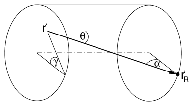
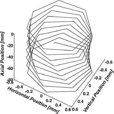
Figure 1: (a) Definition of the angles for a skew ray. The axial angle of the ray is $\theta$. The angle between the projection of the ray in a plane perpendicular to the axis of the fibre with respect to the normal at the point of reflection, $\gamma$, defines the ray’s “skewness”. The angle of incidence at the point of reflection is $\alpha$. (b) The helical path of a skew ray.

For the further discussion in this paper it is convenient to use the axial angle, $\theta$, as given by the supplement of $\theta^{\prime}$, and the skew angle, $\gamma$, to characterise any light ray in terms of its orientation, see figure 1.

The flux transmitted by a fibre is determined by an integration over the angular distribution of the light emitted within the acceptance domain, i.e. the phase space of possible propagation modes. Using an expression given by Potter [9] and setting the transmission function which parameterises the light attenuation to unity, the light flux can be written as follows:

$$\eqalign{F&=F_{m}+F_{s}\\ &=4\rho^{2}\int_{\theta=0}^{\theta_{\it crit}}\int_{\gamma=0}^{\pi/2}\int_{\phi=0}^{\pi/2}I(\theta,\phi)\,\cos^{2}{\gamma}\,d\gamma\,d\Omega\,+\\ &4\rho^{2}\int_{\theta=\theta_{\it crit}}^{\pi/2}\int_{\gamma=\overline{\gamma}(\theta)}^{\pi/2}\int_{\phi=0}^{\pi/2}I(\theta,\phi)\,\cos^{2}{\gamma}\,d\gamma\,d\Omega,}$$ (1)

where $\Omega$ is the element of solid angle, $\overline{\gamma}(\theta)$ refers to the maximum axial angle allowed by the critical angle condition, $\rho$ is the radius of a cylindrical fibre and $I(\theta,\phi)$ is the angular distribution of the emitted light in the fibre core. The two terms, $F_{m}$ and $F_{s}$, refer to either the meridional or skew cases, respectively. The lower limit of the integral for $F_{s}$ is $\overline{\gamma}=\arccos{(\sin{\theta_{\it crit}}/\sin{\theta})}$.

The trapping efficiency for forward propagating photons, $\Omega^{1/2}$, may be defined as the fraction of totally internally reflected photons. The formal expression for the trapping efficiency, including skew rays, is derived by dividing the transmitted flux by the total flux through the cross-section of the fibre core, $F_{0}$. For isotropic emission of fluorescence light the total flux equals $4\pi^{2}\rho^{2}I_{0}$. Then, the first term of equation (1) gives the trapping efficiency in the meridional approximation,

$$\Omega^{1/2}_{m}=F_{m}/F_{0}=\frac{1}{2}(1-\cos{\theta_{\it crit}}),$$ (2)

where all photons are considered to be trapped if $\theta\leq\theta_{\it crit}$, independent of their actual skew angles. The latter formula yields a trapping efficiency of $\Omega^{1/2}_{m}=$ 3.44% for standard plastic fibres with $n_{\it core}=$ 1.6 and $n_{\it clad}=$ 1.49.

The integration of the second term of equation (1) gives the contributions of all skew rays to the trapping efficiency. Integrating by parts, one gets

$$\Omega^{1/2}_{s}=\frac{1}{2}\cos{\theta_{\it crit}}-\frac{\cos^{2}{\theta_{\it crit}}\sin{\theta_{\it crit}}}{2\pi}\int_{0}^{1}\frac{dt}{\sqrt{(1-t)\,t}\,\left(1-t\cos^{2}{\theta_{\it crit}}\right)},$$ (3)

with $t=\cos^{2}{\theta}/\cos^{2}{\theta_{\it crit}}$. Complex integration leads to the result:

$$\Omega^{1/2}_{s}=\frac{1}{2}(1-\cos{\theta_{\it crit}})\cos{\theta_{\it crit}}.$$ (4)

This integral evaluates to 3.20% for standard plastic fibres. The total initial trapping efficiency is then:

$$\Omega^{1/2}=\frac{1}{2}(1-\cos^{2}{\theta_{\it crit}}),$$ (5)

which is 6.64% for standard plastic fibres, i.e. approximately twice the trapping efficiency in the meridional approximation. Nevertheless, for long fibres the effective trapping efficiency is closer to $\Omega^{1/2}_{m}$ than to $\Omega^{1/2}$ since skew rays have a much longer optical path length and therefore get attenuated more quickly see Section 4 for a quantitative analysis.

3 Description of the Photon Tracking Code

The simulation code is written in Fortran. Light rays are generally represented as lines and determined by two points, $\vec{r}$ and $\vec{r}^{\,\prime}$. The points of incidence of rays with the fibre-cladding boundary are determined by solving the appropriate systems of algebraic equations. In the case of a straight fibre the geometrical representation of a straight cylinder is used resulting in the quadratic equation

$$(x+(x^{\prime}-x)\times m)^{2}+(y+(y^{\prime}-y)\times m)^{2}-\rho^{2}=0,$$ (6)

where $\rho$ is the fibre radius and the fibre axis is along the $z$-direction. The positive solution for the parameter $m$ defines the point of incidence, $\vec{r}_{R}$, on the cylinder wall. In the case of a fibre curved in a circular path, the cylinder equation is generalised by the torus equation

$$\eqalign{\left(R-\sqrt{(x+(x^{\prime}-x)\times m+R)^{2}+(z+(z^{\prime}-z)\times m)^{2}}\right)^{2}+\\ (y+(y^{\prime}-y)\times m)^{2}-\rho^{2}=0,}$$ (7)

where the fibre is bent in the $xz$-plane with a radius of curvature $R_{\it curve}$. The roots of this fourth degree polynomial are calculated using Laguerre’s method [10]. It requires complex arithmetic and an estimate for the root to be found. The initial estimate is given by the intersection point of the light ray and a straight cylinder that has been rotated and translated to the previous reflection point. The smallest positive, real solution for $m$ is then used to determine the reflection point, $\vec{r}_{R}$.

In both cases the angle of incidence, $\alpha$, is given by $\cos{\alpha}=\vec{r}_{in}\cdot\vec{n}$, where $\vec{n}$ denotes the unit vector normal to the fibre-cladding boundary at the point of reflection and $\vec{r}_{in}=(\vec{r}-\vec{r}_{R})/|\vec{r}-\vec{r}_{R}|$ is the unit incident propagation vector. The unit propagation vector after reflection, $\vec{r}_{\it out}$, is then calculated by mirroring $\vec{r}_{in}$ with respect to the normal vector: $\vec{r}_{\it out}=\vec{r}_{in}-2\vec{n}\cos{\alpha}$.

4 Results of the Photon Tracking Code

Figure 1 shows the passage of a skew ray along a straight fibre. The light ray has been generated off-axis with an axial angle of $\theta=0.42$ and would not be trapped if it were meridional. The figure illustrates the preservation of the skew angle, $\gamma$, during the propagation of skew rays.

4.1 Trapping Efficiency and Acceptance Domain

Figure 2 shows the total acceptance domain and its splitting into the meridional and skew regions in the meridional ray approximation. The figure gives the values for the two trapping efficiencies which can be determined by integrating over the two angular regions. The integrals are identical in value to formulae 2 and 4, when the photons are generated randomly on the cross-section of the fibre with an isotropic angular distribution in the forward direction.

A skew ray can be totally internally reflected at larger angles $\theta$ than meridional rays and the relationship between the minimum permitted skew angle, $\overline{\gamma}$, at a given axial angle, $\theta$, is determined by the critical angle condition: $\cos{\overline{\gamma}}=\sin{\theta_{\it crit}}/\sin{\theta}$. Inside this region the phase space density is not constant but increases with $\cos{\gamma}^{2}$ and $\sin{\theta}$.

It is obvious from the critical angle condition that a photon emitted close to the cladding has a higher probability to be trapped than when emitted close to the centre of the fibre. Figure 3 shows the trapping efficiency as a function of the radial position, $\hat{\rho}$, of the light emitter in the fibre core. The trapping efficiency is almost independent of the radial position for $\hat{\rho}<0.8$ and the meridional approximation, exactly valid only at $\hat{\rho}=0$, is a good estimate. At $\hat{\rho}\geq 0.9$ the approximation significantly underestimates the trapping efficiency. This fact has been discussed before, e.g. in [11]. Figure 3 shows the the trapping efficiency as a function of the axial angle. All photons with axial angles below $\theta_{\it crit}$ are trapped in the fibre, whereas photons with larger angles are trapped only if their skew angle exceeds the minimum permitted skew angle. It can be seen that the trapping efficiency falls off very steeply with the axial angle.

4.2 Light Attenuation

A fibre can conveniently be characterised by its attenuation length over which the signal amplitude is attenuated to 1$/e$ of its original value. However, light attenuation has many sources, among them self-absorption, optical non-uniformities, reflection losses and absorption by impurities.

Restricting the analysis to the two main sources of loss, the transmission through a fibre can be represented for any given axial angle by $T=\exp\left[-P(\theta)L_{F}/\lambda\right]\,\times q^{\eta L_{F}}$, where the first term describes light losses due to bulk absorption and scattering, and the second term describes light losses due to imperfect reflections which can be caused by a rough surface or variations in the refractive indices. A comparison of some of our own measurements to determine the attenuation length of plastic fibres with other available data indicates that a reasonable value for the bulk absorption length is $\lambda\sim 3$ m. Most published data suggest a deviation of the reflection coefficient, which parameterises the internal reflectivity, from unity between $5\times 10^{-5}$ and $6.5\times 10^{-5}$ [12]. Only for very small diameter fibres ($\sim 10\,\mu$m) are the resulting scattering lengths of the same order as the absorption lengths. Because of the large radii of the fibres discussed reflection losses are not relevant for the transmission function. A reasonable value of $q=0.9999$ is used in the simulation to account for all losses proportional to the number of reflections.

Internal reflections being less than total give rise to so-called “leaky” or non-guided modes, where part of the electromagnetic energy is radiated away at the reflection points. They populate a region defined by axial angles above the critical angle and skew angles slightly larger than the ones for totally internally reflected photons. These modes are taken into account by using the well known Fresnel reflection formulas, where unpolarised light is assumed and the reflection coefficients for the two planes of polarisation are averaged. However, it is obvious that non-guided modes are lost quickly.

The absorption and emission processes in fibres are spread out over a wide band of wavelengths and the attenuation is known to be wavelength dependent. For simplicity only monochromatic light is assumed in the simulation and highly wavelength-dependent effects like Rayleigh scattering are not included explicitly. Light rays are tracked in the fibre core only and no tracking takes place in the surrounding cladding. In long fibres cladding modes will eventually be lost, but for lengths $<1$ m they can contribute to the transmission function and will lead to a dependence of the attenuation length on the distance from the excitation source.

A question of practical importance for the estimation of the light output of a particular fibre application is its transmission function. In the meridional approximation and substituting $\exp(-\ln{q})$ by $\exp(1-q)$ the attenuation length can be written as

$$\Lambda_{m}=-\sec{\theta_{\it crit}}L_{F}\left[1/\lambda+(1-q)\sin{\theta_{\it crit}}/2\rho\right],$$ (8)

which evaluates to $\Lambda_{m}=2.8$ m for the given attenuation parameters. The correct transmission function can be found by integrating over the normalised path length distribution (which will be discussed in the following section):

$$T=\frac{1}{N}\int_{P=0}^{\infty}dN/dP\,e^{-PL/\lambda}\,dP.$$ (9)

Figure 4 shows this transmission function versus the ratio of fibre to absorption length, $L_{F}/\Lambda_{m}$. A simple exponential fit, $T\propto\exp\left[-L_{F}/\Lambda_{\it eff}\right]$, applied to the points results in an effective attenuation length of $\Lambda_{\it eff}=2.4$ m. This description is sufficient to parameterise the transmission function for $L_{F}/\Lambda_{m}\geq 0.2$, at lower values the light is attenuated faster. The difference of order 15% to the meridional attenuation length is attributed to the tail of the path length distribution.

4.3 Propagation of Photons

The analysis of trapped photons is based on the total photon path length per axial fibre length, $P$, the number of internal reflections per axial fibre length, $\eta$, and the optical path length between successive internal reflections, $l_{R}$, where we follow the nomenclature of Potter and Kapany. It should be noted that these three variables are not independent: $P=\eta\times l_{R}$.

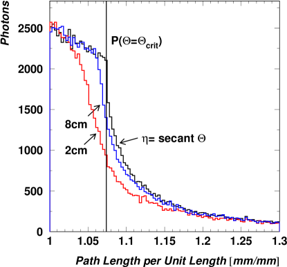
Figure 5: The distribution of the optical path length, $P(\theta)$, of trapped photons in fibres of radius $\rho=$ 0.6 mm normalised to the axial length of the fibre. The figure shows $P(\theta)$ for a straight fibre and for two different radii of curvature, $R_{\it curve}=$ 2 and 8 cm. The vertical line at $P(\theta_{\it crit})=$ 1.074 indicates the upper limit of $P$ in the meridional approximation.

Figure 5 shows the distribution of the normalised optical path length, $P(\theta)$, for photons reaching the exit end of straight and curved fibres of 0.6 mm radius. The figure also gives results for curved fibres of two different radii of curvature. The distribution of path lengths shorter than the path length for meridional photons propagating at the critical angle is almost flat. It can easily be shown that the normalised path length along a straight fibre is given by the secant of the axial angle and is independent of other fibre dimensions: $P(\theta)=\sec\theta$. In case of the curved fibre the normalised path length of the trapped photons is less than the secant of the axial angle and photons on near meridional paths are refracted out of the fibre most.

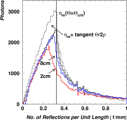
Figure 6: The distribution of the number of reflections, $\eta(\theta)$, for trapped photons in fibres of radius $\rho=$ 0.6 mm normalised to the axial length of the fibre. The figure shows $\eta(\theta)$ for a straight fibre and for two different radii of curvature, $R_{\it curve}=$ 2 and 8 cm. The vertical line at $\eta_{m}(\theta_{\it crit})=$ 0.326 indicates its upper limit in the meridional approximation. The dashed line shows the distribution of $\eta_{m}(\theta)=\tan{\theta}/2\rho$.

The distribution of the normalised number of reflections, $\eta(\theta)$, for photons reaching the exit end of straight and curved fibres is shown in figure 6. Again, the figure gives results for curved fibres of two different radii of curvature. The number of reflections a photon experiences scales with the reciprocal of the fibre radius. In the meridional approximation the normalised number of reflections is related by simple trigonometry to the axial angle and the fibre radius: $\eta_{m}(\theta)=\tan{\theta}/2\rho$. The distribution of $\eta_{m}$, based on the distribution of axial angles for the trapped photons, is represented by the dashed line. The upper limit, $\eta(\theta_{\it crit})$, is indicated in the plot by a vertical line. The number of reflections made by a skew ray, $\eta_{s}(\theta)$, can be calculated for a given skew angle: $\eta_{s}(\theta)=\eta_{m}(\theta)/\cos{\gamma}$. It is clear that this number increases significantly if the skew angle increases. From the distributions it can be seen that in curved fibres the trapped photons experience fewer reflections on average.

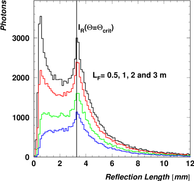
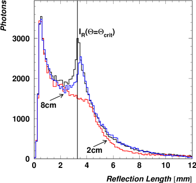
Figure 7: The distribution of the reflection length, $l_{R}(\theta)$, for photons reaching the exit end of fibres of radius $\rho=$ 0.6 mm. The figure shows $l_{R}(\theta)$ for straight fibres (a) with three different fibre lengths, $L_{F}=$ 0.5, 1, 2 and 3 m and for curved fibres (b) with radii of curvature $R_{\it curve}=$ 2 and 8 cm. The vertical line at $l_{R}(\theta_{\it crit})=$ 3.29 mm indicates the lower limit of $l_{R}$ in the meridional approximation.

Figure 7 shows the distribution of the reflection length, $l_{R}(\theta)$, for photons reaching the exit end of fibres of radius $\rho=0.6$ mm. The reflection length will scale with the fibre radius. The left figure shows $l_{R}(\theta)$ for three different over-all fibre lengths and the attenuation behaviour of the photons is made apparent by the non-vanishing attenuation parameters used. Short reflection lengths correspond to long optical path lengths and large numbers of reflections. Because of the many reflections and the long total paths traversed, these photons will be attenuated faster than photons with larger reflection lengths. This reveals the high attenuation of rays with large skew angles. In the meridional approximation the reflection length is related to the axial angle by: $l_{R}=2\rho/\cos{\theta}$. In the figure the minimum reflection length allowed by the critical angle condition is shown by a vertical line at $l_{R}(\theta_{\it crit})=3.29$ mm. The right figure shows $l_{R}(\theta)$ in sharply curved fibres of two different radii of curvature. It can be seen that the region of highest attenuation is close to the reflection length for photons propagating at the critical angle. On average photons propagate with smaller reflection lengths along the curved fibre.

In contrast to the analysis of straight fibres an approximation of the sharply curved fibre by meridional rays is not a very good one, since only a very small fraction of the light rays have paths lying in the bending plane. It is clear that when a fibre is curved the path length, the number of reflections and the reflection length of a particular ray in the fibre are affected, which is clearly seen in Figs. 5, 6 and 7, where the over-all fibre length is 50 cm. The average optical path length and the average number of reflections in a fibre curved over a circular arc are less than those for the same ray in a straight fibre for those photons which remain trapped.

4.4 Trapping Efficiency and Losses in Sharply Curved Fibres

One of the most important practical issues in implementing optical fibres into compact particle detector systems are macro-bending losses. In general, some design parameters of fibre applications, especially if the over-all size of the detector system is important, depend crucially on the minimum permissible radius of curvature. By using the waveguide analysis a loss formula in terms of the Poynting vector can be derived [13], but studies on bending losses in single-mode fibres cannot be directly applied to large diameter fibres. By using ray optics for those fibres the analysis of the passage of skew rays along a curved fibre becomes highly complex.

The angle of incidence of a light ray at the tensile (outer) side of the fibre is always smaller than at the compressed side and photons propagate either by reflections on both sides or in the extreme meridional case by reflections on the tensile side only. If the fibre is curved over an arc of constant radius of curvature photons can be refracted, and will then no longer be trapped, at the very first reflection point on tensile side. Therefore, the trapping efficiency for photons entering a curved section of fibre towards the tensile side is reduced most. Figure 8 quantifies the dependence of the trapping efficiency on the azimuthal angle between the bending plane and the photon path for a curved fibre with a radius of curvature $R_{\it curve}=$ 2 cm.

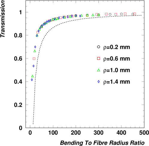
Figure 9: Characteristics of bending losses in curved fibres. The transmission function for fibres curved over a circular arc of 90 ^∘ is plotted as a function of the radius of the curvature to fibre radius ratio for different fibre radii, $\rho=$ 0.2, 0.6, 1.0 and 1.4 mm. The dashed line is a simple estimate from the meridional approximation.

Figure 9 displays the explicit dependence of the transmission function for fibres curved over circular arcs of 90^∘ on the radius of curvature to fibre radius ratio for different fibre radii, $\rho=$ 0.2, 0.6, 1.0 and 1.2 mm. No further light attenuation is assumed. Evidently, the number of photons which are refracted out of a sharply curved fibre increases very rapidly with decreasing radius of curvature. The losses are dependent only on the ratio, since no inherent length scale is involved, justifying the introduction of the curvature to fibre radius ratio as a scaling variable. The light loss due to bending of the fibre is about 10% for a radius of curvature of 65 times the fibre radius.

In the meridional approximation in the bending plane a cut-off angle

$$\cos\theta_{\it cut}=\frac{R+2\rho}{R+\rho}\cos\theta_{\it crit}$$ (10)

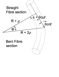
Figure 10: Extreme geometric condition for the trapping of a photon in a curved fibre with radius $\rho$ and radius of curvature $R_{\it curve}$.

can be introduced so that photons emitted with this axial angle $\cos\theta_{\it cut}$ are reflected at the tensile side of the fibre with the critical angle. Figure 10 shows the passage of this meridional ray through the fibre. Reference [14] makes a comparison of the meridional approximation with the waveguide analysis and justifies its use. A transmission function can be estimated from this cut-off angle by assuming that all photons with axial angles $\theta>\theta_{\it cut}$ are refracted out of the fibre:

$$T=1-\frac{1}{1+R_{\it curve}/\rho}\ \frac{\cos\theta_{\it crit}}{1-\cos\theta_{\it crit}}.$$ (11)

This transmission function is shown in figure 9 and it is obvious that it is overestimating the light losses, because of the larger axial angles allowed for skew rays.

The first point of reflection for photons entering a curved section of fibre can be characterised by the bending angle, $\Phi$, through which the fibre is bent. Close to the critical angle the angular phase space density is highest. For photons emitted towards the tensile side the corresponding bending angle is related to the axial angle of the photon, $\Phi=\theta_{\it crit}-\theta_{\it cut}$. For a fibre radius $\rho=$ 0.6 mm and radii of curvature $R_{\it curve}=$ 1, 2, and 5 cm the above formula leads to bending angles $\Phi=$ 0.19, 0.08 and 0.03 rad, respectively.

Photons emitted from the fibre axis towards the compressed side are not lost at this side, however, they experience at least one reflection on the tensile side if the bending angle exceeds the limit $\Phi_{\it limit}=\arccos\left[R_{\it curve}/(R_{\it curve}+2\,\rho)\right]\approx\arccos\left[1-2\,\rho/R_{\it curve}\right]$. A change in the transmission function should occur at bending angles between $\Phi_{\it limit}/2$, where all photons emitted towards the tensile side have experienced a reflection, and $\Phi_{\it limit}$, where this is true for all photons. Figure 11 shows the transmission as a function of bending angle, $\Phi$, for the same fibre conditions as before. Once a sharply curved fibre with a ratio $R_{\it curve}/\rho>83$ is bent through angles $\Phi\sim\pi/8$ rad light losses do not increase any further. The limiting angles range from $\Phi_{\it limit}=1.06$ rad to $\Phi_{\it limit}=0.44$ rad and are indicated in the figure by arrows. At much smaller ratios $R_{\it curve}/\rho$ the meridional approximation is no longer valid to describe this initial behaviour.

Contours of phase space distributions for photons refracted out of sharply curved fibres with radii of curvature $R_{\it curve}=$ 2 and 5 cm are shown in figure 2. The contours demonstrate that skew rays from a small region close to the $\cos{\overline{\gamma}}$ curve are getting lost. The smaller the radius of curvature, the larger the affected phase space region.

4.5 Light Dispersion

A pulse of light, consisting of several photons propagating along a fibre, broadens in time. In active fibres, three effects are responsible for the time distribution of photons reaching the fibre exit end. Firstly the decay time of the fluorescent dopants, usually of the order of a few nanoseconds, secondly the wavelength spectrum of the emitted light, which leads to different propagation velocities for different photons in a dispersive medium, and thirdly the fact that photons on different paths have different transit times to reach the fibre exit end, known as inter-modal dispersion. The timing resolution of scintillators are often of paramount importance.

The transit time in ray optics is simply given by $\tau=P(\theta)/c_{\it core}$, where $c_{\it core}$ is the speed of light in the fibre core. The simulation results on the transit time are shown in figure 12. The full widths at half maximum (FWHM) of the pulses in the time spectrum are presented for four different fibre lengths. The resulting dispersion has to be compared with the time dispersion in the meridional approximation which is simply the difference between the shortest transit time $\tau(\theta=0)$ and the longest transit time $\tau(\theta=\theta_{\it crit})$: $\Delta\tau=L_{F}(\sec{\theta_{\it crit}}-1)/c_{\it core}$, where $L_{F}$ is the total axial length of the fibre. The dispersion evaluates for the different fibre lengths to 197 ps for 0.5 m, 393 ps for 1 m, 787 ps for 2 m and 1181 ps for 3 m. Those numbers are in good agreement with the simulation, although there are tails associated to the propagation of skew rays. With the attenuation parameters of our simulation the fraction of photons arriving later than $\tau(\theta=\theta_{\it crit})$ decreases from 37.9% for a 0.5 m fibre to 32% for a 3 m fibre due to the stronger attenuation of the skew rays in the tail.

5 Summary

We have simulated the propagation of photons in straight and curved optical fibres. The simulations have been used to evaluate the loss of photons propagating in fibres curved in a circular path in one plane. The results show that loss of photons due to the curvature of the fibre is a simple function of radius of curvature to fibre radius ratio and is $<10\%$ if the ratio is $>65$. The simulations also show that for larger ratios this loss takes place in the initial stage of the bend ($\Phi\sim\pi/8$) during which a new distribution of photon angles is established. The photons which survive this initial loss then propagate without further bending losses.

We have also used the simulation to investigate the dispersion of transit times of photons propagating in straight fibres. For fibre lengths between 0.5 and 3 m we find that approximately two thirds of the photons arrive within the spread of transit times which would be expected from the use of the simple meridional ray approximation and the refractive index of the fibre core. The remainder of the photons arrive in a tail at later times due to their helical paths in the fibre. The fraction of photons in the tail of the distribution decreases only slowly with increasing fibre length and will depend on the attenuation parameters of the fibre.

We find that when realistic bulk absorption and reflection losses are included in the simulation for a straight fibre, the overall transmission can not be described by a simple exponential function of propagation distance because of the large spread in optical path lengths between the most meridional and most skew rays.

We anticipate that these results on the magnitude of bending losses will be of use for the design of particle detectors incorporating sharply curved active fibres.

References

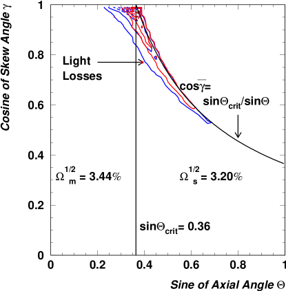
Figure 2: The angular phase space domain for trapped photons in a fibre. To the left of the dividing line at $\sin{\theta_{\it crit}}$ all skew angles are accepted. To the right of the line the maximum skew angle permitted by the critical angle condition is given by $\cos{\overline{\gamma}}=\sin{\theta_{\it crit}/\sin{\theta}}$. The trapping efficiencies are evaluated by integration over the two regions. Contours of phase space distributions for photons refracted out of sharply curved fibres with radii of curvature $R_{\it curve}=$ 2 and 5 cm are shown.

Figure 3: Trapping efficiency for photons propagating in the forward direction as a function of radial position, $\hat{\rho}$, of the light emitter in the fibre core (a) and of the axial angle (b). The maximum axial angle allowed by the critical angle condition in the meridional approximation is indicated.

Figure 4: Simulated transmission function for a straight fibre with a bulk light absorption length $\lambda=$ 3 m and a reflection coefficient $q=$ 0.9999. The transmission as a function of the ratio of fibre to absorption length, $L_{F}/\Lambda_{m}$, is calculated from the optical path length distribution. A simple exponential fit results in an effective attenuation length of $\Lambda_{\it eff}=$ 2.4 m. The dashed line shows the transmission function in the meridional approximation with $\Lambda_{m}=$ 2.8 m.

Figure 8: Trapping efficiencies for photons in a sharply curved fibre with radius of curvature $R_{\it curve}=$ 2 cm and fibre radius $\rho=$ 0.6 mm. The trapping efficiency is plotted as a function of the angle between the photon path and the bending plane, so that 0 rad corresponds to photons emitted towards the tensile side of the fibre.

Figure 11: Simulated transmission function for a curved fibre of radius $\rho=$ 0.6 mm with three different radii of curvature, $R_{\it curve}=$ 1, 2 and 5 cm, corresponding to the ratios $R_{\it curve}/\rho=$ 17, 33 and 83, respectively. The ordinate is the fraction of photons reaching the fibre exit end as a function of the bending angle, $\Phi$, and the arrows indicate angles, $\Phi_{\it limit}$, where in the bending plane a change in the transmission function should occur.

Figure 12: The distribution of the transit time in nanoseconds for photons reaching the fibre exit end. For the fibre lengths $L_{F}=$ 0.5, 1, 2 and 3 m the pulse dispersion (FWHM) of the transit time distribution is 200, 400, 775, and 1200 ps, respectively.

References

- [1] Leutz H, Scintillating fibres, Nucl. Instr. and Meth. in Phys. Res. A364 (1995) 422–448.
- [2] Snitzer E, Cylindrical dielectric waveguide modes, J. Opt. Soc. Am. 51 (5) (1961) 491–498.
- [3] Kapany N S, Burke J J and Shaw C C, Fiber optics. X. Evanescent boundary wave propagation, J. Opt. Soc. Am. 53 (8) (1963) 929–935.
- [4] Kapany N S, Fiber optics. I. Optical properties of certain dielectric cylinders, J. Opt. Soc. Am. 47 (5) (1957) 413–422.
- [5] Kapany N S, Fibre Optics: Principles and Applications, Academic Press, London and New York, 1967.
- [6] Allan W B, Fibre Optics: Theory and Practice, Optical Physics and Engineering, Plenum Press, London and New York, 1973.
- [7] Potter R J, Transmission properties of optical fibers, J. Opt. Soc. Am. 51 (10) (1961) 1079–1089.
- [8] Kapany N S and Capellaro D F, Fiber optics. VII. Image transfer from Lambertian emitters, J. Opt. Soc. Am.51 (1) (1961) 23–31, (appendix: Geometrical optics of straight circular dielectric cylinder).
- [9] Potter R J, Donath E and Tynan R, Light-collecting properties of a perfect circular optical fiber, J. Opt. Soc. Am. 53 (2) (1963) 256–260.
- [10] Press W H, Teukolsky S A, Vetterling W T and Flannery B P, Numerical Recipes in Fortran77: The Art of Scientific Computing, 2nd Edition, Vol. 1 of Fortran Numerical Recipes, Cambridge University Press, 1992.
- [11] Johnson K F, Achieving the theoretical maximum light yield in scintillating fibres through non-uniform doping, Nucl. Instr. and Meth. in Phys. Res.A344 (1994) 432–434.
- [12] D’Ambrosio C, Leutz H and Taufer M, Reflection losses in polysterene fibres, Nucl. Instr. and Meth. in Phys. Res. A306 (1991) 549–556.
- [13] Marcuse D, Curvature loss formula for optical fibers, J. Opt. Soc. Am. 66 (3) (1976) 216–220.
- [14] Gloge D, Bending loss in multimode fibers with graded and ungraded core index, Appl. Opt. 11 (11) (1972) 2506–2513.