Impedance of a Rectangular Beam Tube with Small Corrugations

Abstract

We consider the impedance of a structure with rectangular, periodic corrugations on two opposing sides of a rectangular beam tube. Using the method of field matching, we find the modes in such a structure. We then limit ourselves to the the case of small corrugations, but where the depth of corrugation is not small compared to the period. For such a structure we generate analytical approximate solutions for the wave number $k$, group velocity $v_{g}$, and loss factor $\kappa$ for the lowest (the dominant) mode which, when compared with the results of the complete numerical solution, agreed well. We find: if $w\sim a$, where $w$ is the beam pipe width and $a$ is the beam pipe half-height, then one mode dominates the impedance, with $k\sim 1/\sqrt{w\delta}$ ($\delta$ is the depth of corrugation), $(1-v_{g}/c)\sim\delta$, and $\kappa\sim 1/(aw)$, which (when replacing $w$ by $a$) is the same scaling as was found for small corrugations in a round beam pipe. Our results disagree in an important way with a recent paper of Mostacci et al. [A. Mostacci et al., Phys. Rev. ST-AB, 5, 044401 (2002)], where, for the rectangular structure, the authors obtained a synchronous mode with the same frequency $k$, but with $\kappa\sim\delta$. Finally, we find that if $w$ is large compared to $a$ then many nearby modes contribute to the impedance, resulting in a wakefield that Landau damps.

Submitted to Physical Review Special Topics–Accelerators and Beams:

High Brightness 2002 Special Edition

I INTRODUCTION

In accelerators with very short bunches, such as is envisioned in the undulator region of the Linac Coherent Light Source (LCLS) LCLS Design Study Group (1998), the wakefield due to the roughness of the beam-tube walls can have important implications on the required smoothness and minimum radius allowed for the beam tube. One model that has been used to study roughness is a cylindrically-symmetric structure with small, rectangular, periodic corrugations. For such a structure, if the depth-to-period ratio of the corrugations is not small compared to 1, it has been found that the impedance is dominated by a single strong mode with wave number $k\sim 1/\sqrt{a\delta}$, with $a$ the structure radius and $\delta$ the depth of corrugation, and loss factor $\kappa=4/a^{2}$ (in Gaussian units) M. Timm, A. Novokhatski, T. Weiland (1998); Bane and Novokhatski (1999).

In a recent report Mostacci et al. A. Mostacci, F. Ruggiero, M. Angelici, M. Migliorati, L. Palumbo, S. Ugoli (2002), studied the impedance of a structure with small, rectangular, periodic corrugations on opposing sides of a rectangular beam tube using a perturbation approach. For a beam tube with width $w$ comparable to height $2a$ the authors find a mode with a similar frequency dependence as in the round case, but with a loss factor that is proportional to the depth of corrugation $\delta$. If this model is meant to represent surface roughness with e.g. $\delta\sim 1$ $\mu$m and $a\sim 1$ cm, then their result implies a factor $\sim 10^{-4}$ smaller interaction strength than was obtained in the earlier cylindrically symmetric calculations. Such a result seems unlikely—we would not expect a huge difference in loss factor when changing from round to rectangular geometry. It is the goal of this paper to resolve this discrepancy and to show that a correct calculation for the rectangular cross section indeed gives a result that differs only by a numerical factor from the round case.

Another motivation for this work is to understand the impedance of two corrugated plates, the limit of our geometry when $w$ becomes large. And although, when $w$ is not large, the geometry is somewhat artificial, it may still be a useful model for some vacuum chamber objects of accelerators, e.g. for the screens in the LHC vacuum chamber A. Mostacci, F. Ruggiero, M. Angelici, M. Migliorati, L. Palumbo, S. Ugoli (2002). And thirdly, we note that fabricating a structure with artificially large corrugations, for the purpose of experimentally studying roughness impedance, may be much easier for the rectangular than the round beam pipe.

In this report we calculate the impedance of the rectangular structure of Mostacci et al.—but not limiting ourselves to small corrugations—using the method of field matching. The solution is written as an infinite homogeneous matrix equation that we truncate to solve numerically. Note that our approach is very similar to that used for the analogous cylindrically symmetric problem in the computer program TRANSVRS Bane and Zotter (1980). Note also that recently, Xiao et al. used a similar method to solve the impedance of the rectangular structure, but with the corrugated surfaces replaced by dielectric slabs L. Xiao, W. Gai, X. Sun (2001). Next, using a perturbation approach applied to the field matching equations we find the analytical solution for the limit of small corrugations. Finally, we compare the analytical to the numerical results.

II FIELD MATCHING

We consider a periodic, rectangular structure with perfectly conducting walls, two periods of which are sketched in Fig. 1. In the horizontal ($x$) direction the structure does not vary, except for walls at $x=\pm w/2$. One period of the structure extends longitudinally to $z=\pm p/2$. This cell can be divided into two regions: Region I, the “tube region”, extends to $y=\pm a$; Region II, the “cavity region”, for $z=\pm g/2$, extends beyond $y=\pm a$ to $y=\pm(a+\delta)$. An exciting point beam moves at the speed of light $c$ from minus to plus infinity along the $z$ axis. We are interested in the steady-state fields excited by the beam, and assume that initial transients have all died down. Note that we will work in Gaussian units throughout.

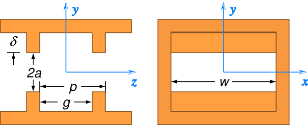
Figure 1: A longitudinal cut of the structure geometry considered here, showing two periods in the $z$-$y$ plane (left), and a transverse cut showing the cross-section of the structure (right).

We assume that the fields of a mode excited by the beam have a time dependence $e^{jkct}$, where $k$ is the mode wave number and $t$ is time. For either region the fields can be obtained from two Hertz vectors, ${\bf\Pi}_{m}$ and ${\bf\Pi}_{e}$, which generate, respectively, TM and TE components of the fields:

$$\cal E = \nabla\times\nabla\times{\bf\Pi}_{m}-jk\nabla\times{\bf\Pi}_{e}\quad,$$ (1)

$$\cal H = \nabla\times\nabla\times{\bf\Pi}_{e}+jk\nabla\times{\bf\Pi}_{m}\quad.$$

Since there is no variation in the $x$ direction we choose it as the direction of the Hertz vectors. To satisfy the boundary conditions at $x=\pm w/2$ the fields vary as cosines and sines of $k_{x}x$ where

$$k_{x}={m\pi\over w}\quad,$$ (2)

with $m$ an odd integer (see below). The general solution involves a summation, over all $m$, of such modes.

Consider modes with horizontal mode number $m$. In the tube region, the most general form of the ($x$ component of the) Hertz vectors, consistent with the (perfectly conducting) walls at $x=\pm w/2$, and the Floquet condition in $z$ is:

$$\Pi_{mx}^{I} = \sum_{n=-\infty}^{\infty}\left[A_{n}\sinh(k_{yn}^{I}y)+B_{n}\cosh(k_{yn}^{I}y)\right]\sin(k_{x}x)\,e^{-j\beta_{n}z}\quad,$$ (3)

$$\Pi_{ex}^{I} = \sum_{n=-\infty}^{\infty}\left[C_{n}\sinh(k_{yn}^{I}y)+D_{n}\cosh(k_{yn}^{I}y)\right]\cos(k_{x}x)\,e^{-j\beta_{n}z}\quad,$$

with

$$\beta_{n}=\beta_{0}+{2\pi n\over p}\quad,\quad\quad{k_{yn}^{I}}=\sqrt{\beta_{n}^{2}-k^{2}+k_{x}^{2}}\quad.$$ (4)

Since the structure is symmetric in $y$ about $y=0$, the field components will be either even or odd in $y$, and the modes will split into two categories. In the first type $A_{n}=D_{n}=0$ and the resulting modes have ${\cal E}_{z}\neq 0$ on axis, in the second type $B_{n}=C_{n}=0$ and the resulting modes have ${\cal E}_{z}=0$ on axis. In either case we are left with only 2 sets of unknown constants in Region I. Since an on-axis beam can only excite modes of the first type, it is this type in which we are interested.

In the cavity region, the most general form of the Hertz potentials, consistent with perfectly conducting boundary conditions at $z=\pm g/2$ and $y=\pm(a+\delta)$ is:

$$\Pi_{mx}^{II} = \sum_{s=1}^{\infty}E_{s}\sin[k_{ys}^{II}(a+\delta-y)]\sin(k_{x}x)\sin[\alpha_{s}(z+g/2)]\quad,$$ (5)

$$\Pi_{ex}^{II} = j\sum_{s=0}^{\infty}F_{s}\cos[k_{ys}^{II}(a+\delta-y)]\cos(k_{x}x)\cos[\alpha_{s}(z+g/2)]\quad,$$

with

$$\alpha_{s}={\pi s\over g}\quad,\quad\quad{k_{ys}^{II}}=\sqrt{k^{2}-\alpha_{s}^{2}-k_{x}^{2}}\quad.$$ (6)

Note that in both regions ${\cal E}_{y}$, ${\cal E}_{z}$, and ${\cal H}_{x}$ depend on $x$ as $\cos(k_{x}x)$ and, therefore, the boundary conditions on the walls at $x=\pm w/2$ are automatically satisfied.

We need to match the tangential electric and magnetic fields in the matching planes, at $y=\pm a$:

$${\cal E}_{z,x}^{I} = \left\{\begin{array}[]{r@{\quad\ :\quad}l}{\cal E}_{z,x}^{II}&\quad\quad\ \ \,|z|<g/2\\ 0&g/2<|z|<p/2\end{array}\right.$$ (9)

$${\cal H}_{z,x}^{I} = \quad{\cal H}_{z,x}^{II}\ \ :\quad\quad\quad\ \,|z|<g/2\quad.$$ (10)

Using the orthogonality of $e^{-j\beta_{n}z}$ over $[-p/2,p/2]$ in Region I, and $\sin[\alpha_{s}(z+g/2)]$ and $\cos[\alpha_{s}(z+g/2)]$ over $[-g/2,g/2]$ in Region II, we obtain a matrix system that we truncate to dimension $2(2{\cal N}+1)\times 2(2{\cal N}+1)$, where ${\cal N}$ is the largest value of $n$ that is kept. To obtain modes excited by the beam we need to set $\beta_{n}=k$ for one value of $n$. The frequencies at which the determinant of the resulting matrix vanishes are the excited frequencies of the structure.

The relation of the coefficients at the excited frequencies gives the eigenfunctions of the modes, from which we can then obtain the $(R/Q)$’s and the loss factors. The loss factor, the amount of energy lost to a mode per unit charge per unit length of structure, is given by

$$\kappa={|{\cal E}_{zs}|^{2}\over 4u(1-v_{g}/c)}\quad,$$ (11)

with ${\cal E}_{zs}$ the synchronous component of the longitudinal field on axis, $u=(8\pi p)^{-1}\int|{\cal E}|^{2}dx\,dy\,dz$, the (per unit length) stored energy in the mode [the integral is over the volume of one period of structure], and $v_{g}$ the group velocity in the mode. Note that the factor $1/(1-v_{g}/c)$ is often neglected in loss factor calculations (it appears to have been neglected in Mostacci et al.). This factor in the loss factor, which—as we will see—is very important in structures with small corrugations, is discussed in Refs. E. Chojnacki, R. Konecny, M. Rosing, J. Simpson (1993); Millich and Thorndahl (1999); Wuensch (1999); we give a new derivation of it in Appendix A. Finally the longitudinal wakefield is given as

$$W(s)=2\Phi(s)\sum_{n}\kappa_{n}\cos(k_{n}s)\quad,$$ (12)

with $\Phi(s)=0$ for $s<0$, $1$ for $s>0$, and the sum is over all excited modes.

In Appendix B we present more details of the calculation of the modes of the corrugated structure using field matching. We have written a Mathematica program that numerically solves these equations for arbitrary corrugation size. The results of this program will be used to compare with small corrugation approximations presented in the following section.

III Small Corrugations

Let us consider the case where the corrugations are small, but with $\delta\sim g\sim p\ll a\sim w$. In the analogous cylindrically symmetric structure it was found that: (i) there is one dominant mode (its loss factor is much larger than those of the other modes), (ii) this mode has a low phase advance per cell, and (iii) the frequency of the mode $k\sim 1/\sqrt{a\delta}$ Bane and Novokhatski (1999); Bane and Stupakov (2000). For our rectangular structure we look for a mode with the same properties. As was the case for the cylindrically symmetric problem we also assume that the fields in the cavity region are approximately independent of $z$, and that one term in the expansion of the $\Pi$ vectors, the term with $n=0$ and $s=0$, suffices to give a consistent solution to the field matching equations Bane and Novokhatski (1999). Note that, it is true that to match the tangential fields well on the matching plane may require many space harmonics (though even then, near the corners, Gibbs phenomena and the edge condition will result in poor convergence); nevertheless, as with the analogous cylindrically symmetric problem, the global mode parameters in which we are most interested—frequency $k$, group velocity $v_{g}$, and loss factor $\kappa$—can be obtained to good approximation when keeping only the one (the $n=0$, $s=0$) term.

Setting $\alpha=0$ implies that $\Pi_{mx}^{II}=0$, and that there are only 3 non-zero field components in the cavity region: ${\cal E}_{z}^{II}$, ${\cal E}_{y}^{II}$, and ${\cal H}_{x}^{II}$. For small corrugations the excited modes become approximately TM modes. To allow matching at the interface of Regions I and II we end up with

$$\Pi_{mx}^{I} \approx 0\quad,$$ (13)

$$\Pi_{ex}^{I} \approx C_{0}\sinh(k_{y0}^{I}y)\cos(k_{x}x)\,e^{-j\beta_{0}z}\quad,$$

and

$$\Pi_{mx}^{II} \approx 0\quad,$$ (14)

$$\Pi_{ex}^{II} \approx jF_{0}\cos[k_{y0}^{II}(a+\delta-y)]\cos(k_{x}x)\quad.$$

Let us sketch how we match the fields: We equate ${\cal E}_{z}$ and ${\cal H}_{x}$ for the two regions at $y=\pm a$; we multiply the first equation by $e^{j\beta_{0}z}$ and integrate over one period in $z$, and then we integrate the second equation over the gap in $z$. When we divide the resulting equations one by the other, the constants $C_{0}$, $F_{0}$, drop out, and we are left with an approximation to the dispersion relation, one valid in the vicinity of the synchronous point (the subscript 0 for $\beta$ is understood):

$$\sqrt{\beta^{2}-k^{2}+k_{x}^{2}}\,\coth\left(\sqrt{\beta^{2}-k^{2}+k_{x}^{2}}\,b\right)={4\sin^{2}({\beta g/2})\over gp\beta^{2}}\sqrt{k^{2}-k_{x}^{2}}\tan\left(\sqrt{k^{2}-k_{x}^{2}}\,\delta\right)\quad.$$ (15)

To properly keep track of the relative size of the terms in further calculations, we assign to each parameter an order using the small parameter $\epsilon$: let $a$, $w$, be of order 1; $\delta$, $g$, $p$, of order $\epsilon^{2}$; and $k$, $\beta$, of order $1/\epsilon$. To find the synchronous frequency we let $\beta=k$ in Eq. (15), expand the equation to lowest order in $\epsilon$, and then set $\epsilon=1$. The result is

$$k^{2}_{m}={k_{x}p\over\delta\,g}\coth\left({k_{x}a}\right)\quad,$$ (16)

(the subscript $m$ is included here to remind us of the $m$ dependence). Note that, if $a\sim w$ (and $p\sim g$) then $k\sim 1/\sqrt{w\delta}$, which is of the same order as the result that was found for the cylindrically symmetric problem. Note also that, for the limit $g=p$, the dispersion relation and the synchronous frequency here agree with those given in Mostacci et al.

For the group velocity we take the partial derivative of Eq. (15) with respect to $\beta$, and rearrange terms to obtain $1-\partial k/\partial\beta=1-v_{g}/c$. After expanding in $\epsilon$, keeping the lowest order term, and finally setting $\epsilon=1$ we obtain

$$\left(1-{(v_{g})_{m}\over c}\right)={2\delta\,k_{x}g\over p}\left[{\sinh^{2}(k_{x}a)\over\sinh(k_{x}a)\cosh(k_{x}a)-k_{x}a}\right]\quad.$$ (17)

Note that, as in the cylindrically symmetric problem, $(1-v_{g}/c)\sim\delta$. The loss factor of our structure

$$\kappa_{m}={2\pi\over wa}F\left({k_{x}a}\right)\quad,$$ (18)

with

$$F(\chi)={\chi\over\sinh(\chi)\cosh(\chi)}\quad.$$ (19)

The function $F(\chi)$ and an approximation for large $\chi$ are shown in Fig. 2. Note that for $\kappa$ in the MKS units of [V/pC/m], one multiplies Eq. (18) by the quantity $Z_{0}c/(4\pi)$, with $Z_{0}=377$ $\Omega$. Note also that our result is independent of $\delta$, unlike the result of Mostacci et al.

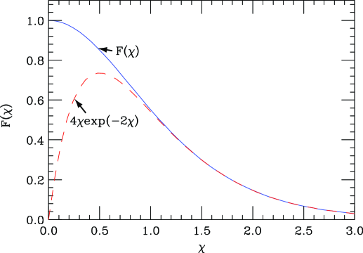
Figure 2: The function $F(\chi)$ (solid) and the approximation $4\chi e^{-2\chi}$, valid for $\chi\gtrsim 1$ (dashes).

The total longitudinal wakefield is given by Eq. (12). Note that, if $w\lesssim a$ ($\chi\gtrsim 1$) then one mode dominates the wake, just like in the round case. (For example, if $\chi=1$, then the amplitude of the first, $m=1$ term is 20 times larger than that of the next, $m=3$ term in the wake sum.) If, however, $w\gg a$, then more than one mode will contribute to the impedance of the structure; in the limit of $w\rightarrow\infty$ (two corrugated plates) there will be a continuum of modes contributing to the impedance. The impedance is given by the Fourier transform of the wake. Its real part is

$${\cal R}{\rm e}Z=\pi\sum_{m}\kappa_{m}\left[\delta(\omega-k_{m}c)+\delta(\omega+k_{m}c)\right]\quad.$$ (20)

Consider now the limit of two corrugated plates ($w\rightarrow\infty$). The mode spectrum becomes continuous and the sum in Eq. (20) can be replaced by an integral

$${\cal R}{\rm e}Z={\pi\over a^{2}}\int_{0}^{\infty}d\chi\,F(\chi)\left[\delta\left(\omega-c\sqrt{{p\over a\delta g}\chi\coth(\chi)}\right)+\delta\left(\omega+c\sqrt{{p\over a\delta g}\chi\coth(\chi)}\right)\right]\quad.$$ (21)

The integral can be solved numerically, with the use of the relation $\int dx\,g(x)\delta[f(x)]=[g(x)/|f^{\prime}(x)|]_{x=x0}$ where $f(x_{0})=0$. The result is shown in Fig. 3a; note that the axes are normalized to $k_{r}=\sqrt{p/(a\delta g)}$ and $Z_{r}=\pi/(a^{2}k_{r}c)$. We see a continuous spectrum of modes beginning at wave number $k_{r}$, with average $1.14k_{r}$ and rms $0.18k_{r}$. The corresponding wakefield becomes a damped oscillation (see Fig. 3b). We see an effective $Q\sim 10$. Note that $W(0^{+})=\pi^{2}/(4a^{2})$ [to be discussed more in a later section].

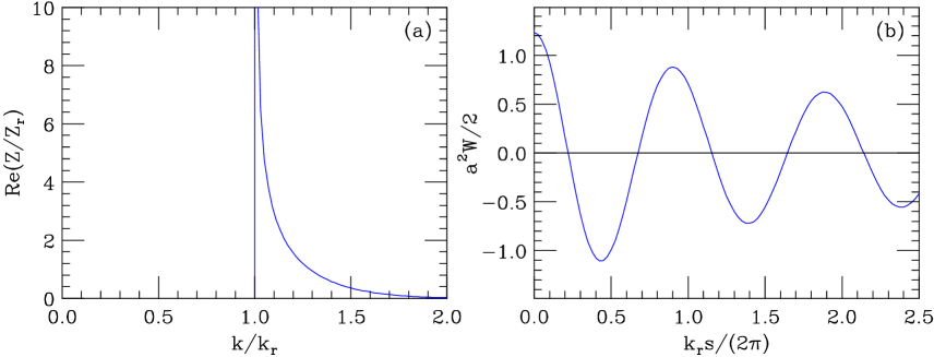
Figure 3: For the case of two corrugated plates ($w\rightarrow\infty$): ${\cal R}{\rm e}(Z)$ (a) and the wake (b), with $k_{r}=\sqrt{p/(a\delta g)}$ and $Z_{r}=\pi/(a^{2}k_{r}c)$.

Finally, we should point out that it has been observed for the case of the cylindrically symmetric problem that, if the small corrugations are replaced by a thin dielectric layer of thickness $\delta$, and if the correspondence is made that the dielectric constant $\epsilon=p/(p-g)$, then the results for the two problems are the same Bane and Novokhatski (1999). Recently the modes in a rectangular structure of Fig. 1, but with the corrugated surfaces replaced by dielectric slabs, have been obtained by Xiao et al., also using a field matching approach L. Xiao, W. Gai, X. Sun (2001). If we take their results, letting the thickness of the dielectric layers ($\delta$) be small, we obtain our results for $k$, $v_{g}$, and $\kappa$ when we make the correspondence $\epsilon=p/(p-g)$.

III.1 Comparison with Numerical Results

To test the validity of the analytical approximations in the case of small corrugations, we compare with numerical results obtained by the Mathematica field matching program (the method of solution is described in Appendix B). Consider as an example a square beam tube ($w/a=2$) with $p/a=0.05$, $g/a=0.025$, and $\delta/a=0.025$, and let us consider the lowest ($m=1$) mode. In the field matching program we take ${\cal S}=4$ and ${\cal N}=4$, i.e. 5 space harmonics are kept in the cavity region and 9 in the tube region. (We find that, for the example geometry, keeping more terms has no significant effect on the results.)

We begin by comparing the dispersion curve (see Fig. 4). Shown are the field matching result (the solid curve) and the approximation, Eq. (15) (the dashes). We see that the two agree well except far from the synchronous phase. The cross plotting symbol locates the synchronous point, with $kp=0.200\pi$, a result which is 7.5% larger than the analytical value of Eq. (16). It is interesting to note that this dispersion curve is almost identical to the one obtained (also by field matching) for the same geometry but in a round beam pipe Bane and Novokhatski (1999). As for the loss factor, we find that it is a factor 0.84 as large as the analytical approximation, Eq. 18.

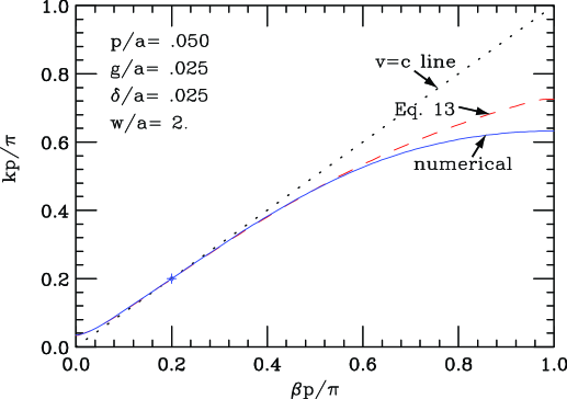
Figure 4: A dispersion curve example: shown are the numerical result (solid), the synchronous point (the cross plotting symbol), and the approximation, Eq. (15) (dashes). Also shown is the speed of light line (dots).

These results confirm the validity of the analytical approximations for the structure with small corrugations, provided that the depth of corrugation $\delta$ is not small compared to the corrugation period $p$. However, in Ref. Bane and Novokhatski (1999) it was shown that for the analogous round structure the corresponding analytical formulas break down when $\delta$ becomes small compared to $p$: as $\delta$ decreases the frequency first increases than decreases as compared to the analytical result; meanwhile the loss factor continually decreases. When $\delta$ is small compared to $p$ the impedance is no longer well characterized by a single resonance, and is best described by a different model Stupakov (2001). As expected, we find the same kind of behavior in our rectangular structure. If, for example, we reduce $\delta$ in our example problem by a factor of 2, we find that the frequency becomes 18% larger, and the loss factor 30% smaller, than the values given by the analytical formulas.

III.2 Discussion

Our result for the loss factor, Eq. (18), is independent of the depth of corrugation $\delta$, as was found previously for the analogous cylindrically symmetric problem Bane and Novokhatski (1999); Bane and Stupakov (2000). This result, however, is in disagreement with the result of Mostacci et al., where the loss factor was found to be directly proportional to $\delta$. This discrepancy is important to resolve.

There is a general relation that holds for the wake directly behind the driving particle

$$W(0^{+})={2\over\pi}\int_{0}^{\infty}{\cal R}{\rm e}Z(\omega)\,d\omega=2\sum_{m}\kappa_{m}\quad,$$ (22)

a relation that does not depend on the specific boundary conditions at the wall. To discuss it, consider first the analogous cylindrically symmetric problem. It was earlier found that, as long as the corrugations are small and the depth $\delta\gtrsim p$, the contribution of one mode dominates the wake sum. In this case, it was found that, as here, $W(0^{+})$ (or $\kappa$) is independent of $\delta$ Bane and Novokhatski (1999). If the corrugations are replaced by a thin dielectric layer, $W(0^{+})$ does not depend on the dielectric properties (neither $\delta$ nor $\epsilon$) Novokhatski and Mosnier (1997). In the same way, if the corrugations are replaced by a lossy metal, $W(0^{+})$ will not depend on the conductivity Chao (1993). And in all three cases the answer is the same: $W(0^{+})=4/a^{2}$. [In fact, this relation is also valid for the (steady-state) wake of a periodic accelerator structure, with $a$ the iris radius Gluckstern (1989); com .]

We expect the same type of behavior to hold in a corrugated, rectangular structure, i.e. that $W(0^{+})$ depends only on the cross-section geometry of the beam pipe. In Fig. 5 we plot, for our rectangular structure, $a^{2}W(0^{+})/2=a^{2}\sum_{m}\kappa_{m}$, as function of $\pi a/w$ (the solid curve). Also shown is the contribution of only the first ($m=1$) term (dashes), and the approximation $8(\pi a/w)^{2}\exp(-2\pi a/w)$ (dots). Note that, for $\pi a/w$ small, many modes contribute to the sum; for $\pi a/w\gtrsim 1$, one mode dominates. As with the cylindrically-symmetric case, $W(0^{+})$ must still be correct if we replace the corrugated surfaces by thin dielectric slabs, or by lossy metal plates. We know of no published result for $W(0^{+})$ in our rectangular geometry to compare with; nevertheless, Henke and Napoly found $W(0^{+})$ between two resistive parallel plates Henke and Napoli (1990), which becomes the limit of our geometry as $w\rightarrow\infty$. Their result, $a^{2}W(0^{+})/2=\pi^{2}/8$, agrees with our calculation for $\pi a/w\rightarrow 0$, and confirms our result.

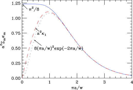
Figure 5: The sum of the loss factors $a^{2}\sum_{m}\kappa_{m}$ [$=a^{2}W(0^{+})/2$] as function of $\pi a/w$ (solid). Also shown are the contribution of the first mode, $a^{2}\kappa_{1}$ (dashes), and the approximation $8(\pi a/w)^{2}\exp(-2\pi a/w)$ (dots).

For a given bunch shape and fixed $\delta/p$, as the depth of corrugation $\delta$ decreases, we expect the induced voltage (the convolution of the bunch shape with the wake) to also decrease. If the loss factor does not depend on $\delta$ how does this happen? The answer is that as $\delta$ decreases, the mode frequency $k$ increases, and the wake, when convolved with the bunch shape, will yield an induced voltage that will decrease (at least as fast as $1/k$). Concerning this question, the wake of this structure behaves similarly to the resistive wall wake for very short bunches as the conductivity increases: $W(0^{+})$ also does not change but the wake first zero crossing moves closer to $s=0$.

IV CONCLUSION

We studied the impedance of a structure with rectangular, periodic corrugations on two opposing sides of a rectangular beam tube using the method of field matching. We described a formalism that, for arbitrary corrugation size, can find the resonant frequencies $k$, group velocities $v_{g}$, and loss factors $\kappa$. In addition, for the case of small corrugations, but where the depth of corrugation is not small compared to the period, we generated analytical perturbation solutions for $k$, $v_{g}$, and $\kappa$ for the dominant mode. We then compared, for such a structure, the results of the computer program and the analytical formulas, and found good agreement.

In general, we found that, for the structure of interest, the results are very similar to what was found earlier for a structure consisting of small corrugations on a round beam pipe: if $w\sim a$, where $w$ is the beam pipe width and $a$ is the beam pipe half-height, then one mode dominates the impedance, with $k\sim 1/\sqrt{a\delta}$ ($\delta$ is the depth of corrugation), $(1-v_{g}/c)\sim\delta$, and $\kappa\sim 1/a^{2}$. If, however, $w$ is large compared to $a$ we find that many nearby modes contribute to the impedance, resulting in a wakefield that Landau damps.

Appendix A Excitation of a synchronous mode by a moving relativistic point charge

Consider first a cavity of frequency $\omega$ with the electric field of an eigenmode $\textnormal{\boldmath$\cal{E}$}(\textnormal{\boldmath$r$})e^{j\omega t}.$ The energy in the eigenmode is denoted by $U$. If a point charge $q$ passes through the cavity, it excites this mode to the amplitude $A_{s}$ (where $A_{s}$ is a complex number), so that after the passage through the cavity the electric field of the mode will be $A_{s}\textnormal{\boldmath$\cal{E}$}(\textnormal{\boldmath$r$})e^{j\omega t},$ and the energy lost by the charge is equal to $|A_{s}|^{2}U$. In quantum language, this is spontaneous radiation of the charge into the mode under consideration which is indicated by the subscript $s$. It is clear that $A_{s}$ is proportional to the charge of the particle $q$.

To calculate the amplitude $A_{s}$, let us consider a situation when, before the charge enters the cavity, the latter already has this mode excited by an external agent (RF source) to the amplitude $A_{0}$. Due to linearity of Maxwell’s equation, after the passage of the charge, the field in the cavity will be equal to the sum of the initial mode $A_{0}$ and the spontaneously radiated mode $A_{s}$, with the energy given by $|A_{s}+A_{0}|^{2}U$. The change of the energy $\Delta W$ in the cavity is

$$\Delta W=|A_{s}+A_{0}|^{2}U-|A_{0}|^{2}U=(A_{s}A_{0}+\mathrm{c.c.})U+|A_{s}|^{2}U\,,$$ (23)

where c.c. denoted a complex conjugate. Let us consider the limit of small charges, $q\rightarrow 0$, then we can neglect the last term on the right hand side of Eq. (23), which scales as $q^{2}$, and keep only the first term that is linear in $q$,

$$\Delta W=(A_{s}A_{0}+\mathrm{c.c.})U\,.$$ (24)

Discarding the term $\propto q^{2}$ means that we neglect the beam loading effect.

We can now balance the energy change $\Delta W$ with the work done by the external field $A_{0}$ during the passage of the charge. This work is equalt to the integral of the electric field ${\cal{E}}_{z}(z)$ along the particle’s orbit

$$\Delta W=-q{\cal R}{\rm e}A_{0}\int dz{\cal{E}}_{z}(z)e^{j\omega z/v}=-\frac{qA_{0}}{2}\int dz{\cal{E}}_{z}(z)e^{j\omega z/v}+\mathrm{c.c.}$$

Comparing Eq. (24) with Eq. (A) we conclude that

$$A_{s}=-\frac{q}{2U}\int dz{\cal{E}}_{z}(z)e^{j\omega z/v}.$$ (25)

Hence we found the amplitude of spontaneous radiation of the particle in terms of the integral along the particle’s orbit of the electric field.

The energy lost by the particle (loss factor) is

$$|A_{s}|^{2}U=\frac{q^{2}|V|^{2}}{4U},$$ (26)

where the voltage $V=\int dz{\cal{E}}_{z}(z)e^{j\omega z/v}$.

Let us now apply the same approach as above to the excitation of a mode that propagates with the speed of light in a waveguide. To deal with a mode of finite energy we consider a wave packet, and assume that the packet has a length $L$, as shown in Fig. 6 below.

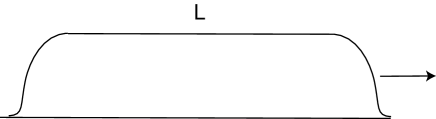
Figure 6: The shape of the wave packet of the synchronous mode. The packet has a long plateau of length $L$ and short edges.

It propagates in the pipe with the group velocity $v_{g}$. The energy in the mode $U$ can be related to the energy flow $P$ (integrated over the cross section averaged over time the Pointing vector) if we note that $U/L$ is the energy per unit length, and hence $(U/L)v_{g}$ is the energy flow equal to $P$, hence

$$U=\frac{PL}{v_{g}}\,.$$ (27)

Now, the particle is synchronous with the wave and stays all the time in the same phase, so it sees the same longitudinal electric field ${\cal{E}}_{z}$ which we denote by ${\cal E}_{zs}$. The integral from Eq. (25) can be written as

$$\int dz{\cal{E}}_{z}(z)e^{j\omega z/v}\rightarrow cT{\cal E}_{zs}\,,$$ (28)

where $T$ is the interaction time between the wave and the particle. This is actually the time when the particle stays in the wave, and taking into account that the wave is moving with velocity $v_{g}$ and the particle is moving with $c$

$$T=\frac{L}{c-v_{g}}.$$ (29)

Hence, for the amplitude of the radiated wave we find

$$A_{s}=-\frac{q}{2U}{\cal E}_{zs}\frac{cL}{c-v_{g}}\,,$$ (30)

and the energy $W$ radiated by the particle

$$W=A_{s}^{2}U=\frac{q^{2}}{4U}{\cal E}_{zs}^{2}\frac{c^{2}L^{2}}{(c-v_{g})^{2}}.$$ (31)

To find the energy radiated per unit length of the path, we divide $W$ by the length of the interaction path $Lc/(c-v_{g})$, which gives

$$\frac{dW}{dz}=\frac{q^{2}}{4u}{\cal E}_{zs}^{2}\frac{c}{(c-v_{g})},$$ (32)

where the energy per unit length of the path $u=U/L$. Finally, since the loss factor $\kappa=q^{-2}dW/dz$, we arrive at Eq. (11).

Appendix B FIELD MATCHING, THE GENERAL SOLUTION

In Section II we presented Hertz vectors and wave numbers for Regions I and II, and also the four equations that need to be matched at the interface $y=\pm a$. We continue with the notation introduced there: We multiply the matching equations for ${\cal E}_{z}$ and ${\cal E}_{x}$ by $e^{j\beta_{n^{\prime}}z}$ and integrate over $[-p/2,p/2]$; and we multiply the matching equations for ${\cal H}_{z}$ and ${\cal H}_{x}$ by $\sin[\alpha_{s^{\prime}}(z+g/2)]$ and $\cos[\alpha_{s^{\prime}}(z+g/2)]$ and integrate over $[-g/2,g/2]$. We obtain the infinite set of equations:

$$(C^{\prime}_{n}kk_{yn}^{I}w-B^{\prime}_{n}m\pi\beta_{n})\cosh(k_{yn}^{I}b) = {g\over p}\sum_{s}N_{ns}(-F^{\prime}_{s}kk_{ys}^{II}w+E^{\prime}_{s}m\pi\alpha_{s})\sin(k_{ys}^{II}\delta)$$

$$-B^{\prime}_{n}\cosh(k_{yn}^{I}b) = {g\over p}\sum_{s}M_{ns}E^{\prime}_{s}\sin(k_{ys}^{II}\delta)$$

$$(E^{\prime}_{s}kk_{ys}^{II}w+F^{\prime}_{s}m\pi\alpha_{s})\cos(k_{ys}^{II}\delta) = 2\sum_{n}M_{sn}(B^{\prime}_{n}kk_{yn}^{I}w-C_{n}m\pi\beta_{n})\sinh(k_{yn}^{I}b)$$

$$(1+\delta_{s0})F^{\prime}_{s}\cos(k_{ys}^{II}\delta) = -2\sum_{n}C^{\prime}_{n}N_{sn}\sinh(k_{yn}^{I}b)\quad.$$ (33)

Here

$$B^{\prime}_{n},C^{\prime}_{n}=jB_{n},jC_{n}\quad,\quad\quad\quad E^{\prime}_{s},F^{\prime}_{s}=\left\{\begin{array}[]{r@{\quad:\quad}l}E_{s},F_{s}&s\ {\rm even}\\ jE_{s},jF_{s}&s\ {\rm odd}\end{array}\right.\ ,$$ (34)

$$\left\{\begin{array}[]{c}N_{ns}\\ M_{ns}\end{array}\right\}=\left\{\begin{array}[]{c}\beta_{n}\\ \alpha_{s}\end{array}\right\}{2\over(\beta_{n}^{2}-\alpha_{s}^{2})g}\left[\begin{array}[]{r@{\quad:\quad}l}\sin(\beta_{n}g/2)&s\ {\rm even}\\ \cos(\beta_{n}g/2)&s\ {\rm odd}\end{array}\right.\ ,$$ (35)

and $\delta_{ss^{\prime}}$ the Kronecker delta.

This system of equations can be written as a homogenous matrix equation:

$$\left[\left(\begin{array}[]{cc}G(H^{2}-I^{2})&-GH\\ -GH&G\end{array}\right)+\left(\begin{array}[]{cc}N&0\\ 0&M\end{array}\right)\left(\begin{array}[]{cc}P(Q^{2}+R^{2})/S&-PQ\\ -PQ/S&P\end{array}\right)\left(\begin{array}[]{cc}N^{T}&0\\ 0&M^{T}\end{array}\right)\right]\left(\begin{array}[]{c}B^{\prime\prime}\\ C^{\prime\prime}\end{array}\right)=0$$ (36)

with superscript $T$ indicating the transpose of a matrix. The diagonal elements of diagonal matrices are: $G_{n}=\coth(k_{yn}^{I}b)/(kk_{yn}^{I}w)$, $H_{n}=m\pi\beta_{n}$, $I_{n}=kk_{yn}^{I}w$; $P_{s}=2g\tan(k_{ys}^{II}\delta)/(pkk_{ys}^{II}w)$, $Q_{s}=m\pi\alpha_{s}$, $R_{s}=kk_{ys}^{II}w$, $S_{s}=(1+\delta_{s0})$. Note that the system matrix is real. The expansion coefficients are: $B_{n}^{\prime\prime}=-\sinh(k_{yn}^{I}b)C^{\prime}_{n}$ and $C_{n}^{\prime\prime}=\sinh(k_{yn}^{I}b)(kk_{yn}^{I}wB^{\prime}_{n}-m\pi\beta_{n}C^{\prime}_{n})$.

To solve the matrix equation we truncate to dimension $2(2{\cal N}+1)\times 2(2{\cal N}+1)$, where ${\cal N}$ is the largest value of $n$ that is kept. Therefore, subscript $n$, representing space harmonic number in the tube region, runs from $-{\cal N}$ to ${\cal N}$; subscript $s$, representing space harmonic number in the cavity region, runs from $0$ to ${\cal S}$, the largest value kept. Note that the values ${\cal N}$, ${\cal S}$, should be chosen so that $(2{\cal N}+1)/p\approx({\cal S}+1)/g$. The system matrix $U$ is a function of $\beta_{0}$ and of $k$. To find synchronous modes, we need to first set, for one space harmonic $n^{\prime}$, $\beta_{n^{\prime}}=k$ and then numerically search for the value of $k$ for which the determinant of $U$ becomes zero. The value $n^{\prime}$ should be taken to be the nearest integer to $kp/(2\pi)$. To find values of the dispersion curve, we, for various values of $\beta_{n^{\prime}}$ [where again $n^{\prime}$ is the nearest integer to $kp/(2\pi)$], numerically search for the value of $k$ for which the determinant of $U$ becomes zero.

Once we have found the frequency we can find the eigenfunctions, from which we obtain $|{\cal E}_{zs}|^{2}$ on axis,

$$|{\cal E}_{zs}|^{2}=k^{2}\left|B_{ns}^{\prime}k_{x}-C_{ns}^{\prime}k_{y}^{I}\right|^{2}\quad,$$ (37)

(where $ns$ represents the synchronous space harmonic) and the energy per unit length $u$. For example, the stored energy in Region I is given by

$$u^{I}={\displaystyle{1\over 32\pi p}}{\displaystyle\sum_{n}}\left(B_{n}^{\prime 2}\left[2k^{2}k^{2}_{-}a+\left(k^{4}_{-}+k_{x}^{2}k_{y}^{I2}+k_{x}^{2}\beta_{n}^{2}\right)\sinh(2k_{yn}^{I}a)/k_{yn}^{I}\right]\right.\quad\quad\quad\quad\quad\quad\quad\quad\quad\quad$$

$$\left.+C_{n}^{\prime 2}\left[-2k^{2}k^{2}_{-}a+\left(k^{2}k_{y}^{I2}+k^{2}\beta_{n}^{2}\right)\sinh(2k_{yn}^{I}a)/k_{yn}^{I}\right]-4B_{n}^{\prime}C_{n}^{\prime}kk_{x}\beta_{n}\sinh(2k_{yn}^{I}a)\right)$$ (38)

with $k_{-}^{2}=k^{2}-k_{x}^{2}$, with a corresponding equation giving the energy stored in Region II. Note that for small corrugations, $u^{II}\ll u^{I}$. The quantity $1/(1-v_{g}/c)$ is obtained by first calculating the dispersion curve, and then finding the slope at the synchronous point numerically. Knowing $|{\cal E}_{zs}|^{2}$, $u$, and $1/(1-v_{g}/c)$ we can finally obtain the loss factor $\kappa$.