Femtosecond Resolution Experiments at Third-Generation Light Sources: a Concept Based on the Statistical Properties of Synchrotron Radiation

Abstract

The paper describes a new concept of visible pump/X-ray probe/slow detector experiments that could be performed at third-generation synchrotron light sources. We propose a technique that would allow time resolution up to femtosecond capabilities to be recovered from a long (100 ps) X-ray probe pulse. The visible pump pulse must be as short as the desired time resolution. The principle of operation of the proposed pump-probe scheme is essentially based on the statistical properties of the synchrotron radiation. These properties are well known in statistical optics as properties of completely chaotic polarized light. Our technique utilizes the fact that, for any synchrotron light beam there exist some characteristic time (coherence time), which determines the time-scale of the random fluctuations. The typical coherence time of soft X-ray synchrotron light at the exit of monochromator is in the femtosecond range. An excited state is prepared with a pump pulse and then projected with a probe pulse onto a final ion state. The first statistical quantity of interest is the variance of the number of photoelectrons detected during synchrotron radiation pulse. The statistics of concern are defined over an ensemble of synchrotron radiation pulses. From a set of variances measured as a function of coherence time (inversely proportional to monochromator bandwidth) it is possible to reconstruct the femtosecond dynamical process.

DESY 02-127

September 2002

, ,

1 Introduction

Time-resolved experiments are used to monitor time-dependent phenomena. The study of dynamics in physical systems often requires time resolution beyond the picosecond capabilities presently available with synchrotron radiation. Femtosecond ($10^{-15}$s) capabilities have been available for many years at visible wavelengths. There exists a wide interest in the extension of femtosecond techniques to the soft X-ray, and X-ray regions of spectrum.

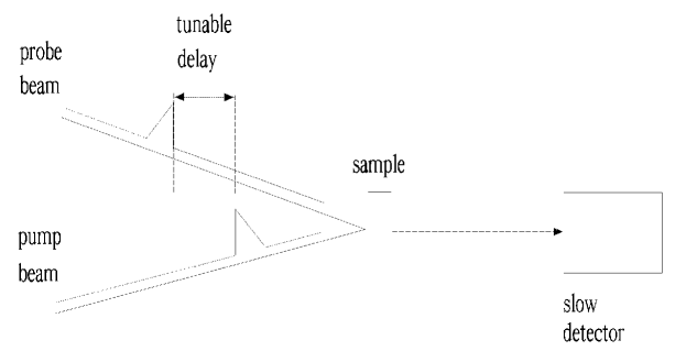
Figure 1: Typical scheme of a ”short pump-short probe” experiment

The time resolution of pump-probe experiment is, obviously, determined by the duration of the pump as well as the resolution of the probing. The pump pulse must always be as short as the desired time resolution. In typical scheme of a pump-probe experiment (see Fig. 1) the short probe pulse follows the pump pulse at some specified delay. The signal recorded by the slow detector then reflects the state of the sample during the brief probing. The experiment must be repeated many times with different delays in order to reconstruct the femtosecond dynamical process [1, 2].

The obvious temporal limitation of the typical visible pump/X-ray probe technique is the duration of the X-ray probe. Here we will concentrate on the performance obtained with third-generation storage rings. At these sources, the X-ray pulse duration is about 100 ps. The new principle of pump-probe techniques described below offers a way around this difficulty. We propose visible pump / X-ray probe technique that would allow time resolution up to femtosecond capabilities to be recovered from a long X-ray probe pulses (see Fig. 2). The principle of operation of the proposed pump-probe scheme is essentially based on the statistical properties of the synchrotron radiation. Synchrotron radiation is a stochastic object and at a given time it is impossible to predict the amount of energy which flows to a sample. For any synchrotron light beam there exist some characteristic time, which determines the time-scale of the random fluctuations. This characteristic time is called, in general, the coherence time $\tau_{\mathrm{c}}$ of the synchrotron light beam. Its magnitude is of the order of the inverse of the frequency spread of the beam. In all the theory that follows, attention is restricted to synchrotron light beams whose frequency spreads are small compared with the mean frequency, that is, where $\omega_{0}\tau_{\mathrm{c}}$ is very much larger than unity. Figure 3 illustrates the type of fluctuations that occur in the synchrotron radiation beam intensity and phase. The figures have been constructed by a computer simulation of a synchrotron light source in which the summation is carried out explicitly for the real number of electrons $(N\simeq 10^{10})$ in the electron bunch. It is seen that substantial changes in intensity (and phase) occur over a time span $\tau_{\mathrm{c}}$, but these quantities are reasonably constant over time intervals $\Delta t\ll\tau_{\mathrm{c}}$.

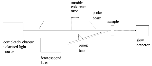
Figure 2: The new scheme of ”pump-probe” experiment. The principle of operation of the proposed scheme is based essentially on the statistical properties of synchrotron radiation, which possesses all the features corresponding completely chaotic polarized light

Figure 3: Time-dependence of the intensity (upper plot) and phase (lower plot) for synchrotron light, obtained from a computer simulation.The dashed line shows the mean value of the intensity averaged over an ensemble of radiation pulses

Our technique utilizes the fact that, over the long probe pulse, time correlations exist in the probe pulse intensity. It was shown that the femtosecond timescale associated with intensity fluctuations in synchrotron light pulses make them well suited for time-resolved studies. The first statistical quantity of interest is the variance of the detector counts. The statistics of concern are defined over an ensemble of synchrotron radiation pulses. From a set of variances measured as a function of correlation time it is possible to reconstruct the femtosecond dynamical process.

2 The principle of pump-probe techniques based on the statistical properties of synchrotron light

The shot noise in the electron beam causes fluctuations of the beam density which are random in time and space. As a result, the radiation, produced by such a beam, has random amplitudes and phases in time and space. These kinds of radiation fields can be described in terms of statistical optics, branch of optics that has been developed intensively during the last few decades and there exists a lot of experience and a theoretical basis for the description of fluctuating electromagnetic fields [3, 4].

We will begin in this section by dealing with some general notions of statistical optics. Some of the statements will be quite precise, other only partially precise. In the framework of statistical optics the radiation field is characterized by notions such as time and space coherence. Let us illustrate these notions. To be specific, we consider the radiation pulse of nearly monochromatic radiation having a duration and bandwidth equal to $T$ and $\Delta\omega$, respectively. If $T\gg 1/\Delta\omega$, the radiation is partially coherent in time. The time coherence is of about $\tau_{\mathrm{c}}\simeq 1/\Delta\omega$. The physical sense of this notion is as follows. Let us separate the radiation pulse by a splitter. These two pulses pass different path lengths and are then combined together. If the difference between the path lengths is less than $c\tau_{\mathrm{c}}$, we see the interference pattern at the end for a shot-to-shot averaging (averaging over a large number of radiation pulses). Using simple physical language, we can say that the radiation field is correlated within the time of coherence.

The notion of space coherence can be explained in the same way. Let us direct the radiation onto a screen with two pinholes and look at the interference pattern in the far diffraction zone when changing the distance between the pinholes. When the pinholes are located close to each other, we see a clear diffraction pattern. As the distance between the holes increases to some value, $D>\Delta r_{\mathrm{c}}$, we come to the situation when we do not see an interference pattern after averaging over the ensemble of pulses. Qualitatively, the value of $\pi(\Delta r_{\mathrm{c}})^{2}$ is referred as the area of coherence of the radiation pulse. The coherence volume is defined as the product of the coherence area, $\pi(\Delta r_{\mathrm{c}})^{2}$, with the coherence length, $c\tau_{\mathrm{c}}$. If one uses the notions of quantum mechanics, this volume corresponds to one cell in the phase space of the photons. The number of photons in the coherence volume is also referred to as the degeneracy parameter, $\delta_{\mathrm{W}}$. Physically this parameter means the average number of photons which can interfere, or the number of photons in one quantum state (one mode). It should be noted that third-generation synchrotron light sources can produce soft X-ray radiation with very high degeneracy parameter and in such cases we can state that the classical approach is adequate for a description of the statistical properties of the synchrotron radiation.

Electron beam is composed of large number of electrons, thus fluctuations always exist in the electron beam density due to the effect of shot noise. When the electron beam enters the undulator, the presence of the beam modulation at frequencies close to the resonance frequency initiates the process of radiation. The shot noise in the electron beam is a Gaussian random process. The monochromator can be considered as a linear filter which does not change the statistics of the signal. As a result, we can define general statistical properties of the radiation after monochromator without any calculations. For instance, the real and imaginary parts of the slowly varying complex amplitudes of the electric field of the electromagnetic wave have a Gaussian distribution, the instantaneous radiation power fluctuates in accordance with the negative exponential distribution, and the energy in the radiation pulse fluctuates in accordance with the gamma distribution. We can also state that the spectral density of the radiation energy and the first-order time correlation function should form a Fourier transform pair (this is so-called Wiener Khintchine theorem). Also, the higher-order correlation functions (time and spectral) should be expressed in terms of the first-order correlation functions. These properties are well known in statistical optics as properties of completely chaotic polarized radiation [4]. This demonstrate one of the most beautiful things about statistical optics - how much can be deduced from so little. This brings up an interesting question: Why is it that the noise in the electron bunch is a Gaussian random process? We will give an explanation in section 3.

The arrangement of components for a long probe pulse experiment is shown in Fig. 4. In order to use the radiation from synchrotron light source it first has to be spatially filtered and monochromatized. We assume that synchrotron radiation reaching the sample surface has full transverse coherence. With this assumption, attention can be concentrated completely on temporal coherence effects. The coherence time of synchrotron light is inversely proportional to the monochromator bandwidth. So the narrower we make the monochromator exit slit, the wider the coherence time gets. Any measurement of photodetector counts will be accompanied by certain unavoidable fluctuations and we wish to determine the statistical distribution of the number of photocounts observed in any radiation pulse.

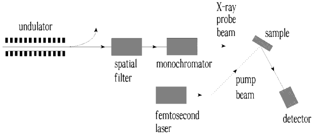
Figure 4: Proposed pump-probe experimental setup

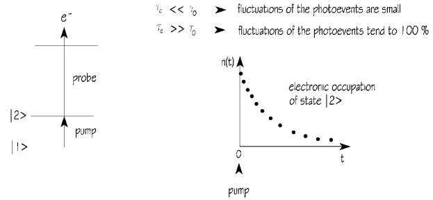
Figure 5: Schematic ionization scheme for pump-probe ionization in the visible pump/X-ray probe transition. A typical experiment would be to couple two electronic state $|1\rangle$ and $|2\rangle$ resonantly by a femtosecond pump-field. The dynamics is then probed by ionization and detection of the fluctuations of photoelectron counts per pulse as a function of the coherence time of the probe synchrotron radiation pulse

Now we wish to consider one example which shows the relationship between the fluctuations of photocounts and the coherence time in a circumstances that easy to understand. We will not discuss applications of the proposed pump-probe scheme. There are, in fact, many applications that could be discussed. We have chosen for emphasis here experiments aimed at measuring the lifetime of electronic excitation in condensed matter. For our present purposes we would like to imagine a somewhat idealized experiment. Several assumptions are made about the process of internal conversion of the electronic excitation. First, the time dependence of the electronic occupation is assumed to be known a priory – this is the exponential dependence $n(t)=n_{0}\exp(-t/\tau_{0})$. In practice, this is a good assumption. The purpose of the measurement is presumably to determine the lifetime $\tau_{0}$. The typical lifetime of the electronic excitation is in the femtosecond range. This type of time-resolved experiments may be understood as preparing an excited state with a pump pulse and then projecting it with a probe pulse onto a final state. The final state should be well characterized. Photoionization detection has several advantages. The ion state may be well characterized by independent methods such as high resolution photoelectron spectroscopy. Schematic ionization scheme for pump-probe ionization is illustrated in Fig. 5. A typical experiment would be to couple two electronic state $\mid 1\rangle$ and $\mid 2\rangle$ resonantly by a femtosecond pump-field at a frequency $\omega$ in the visible range. The dynamics is then probed by ionization and detection of the photoelectrons as a function of the coherence time of the probe synchrotron radiation pulse. A time-resolved experiment inherently begins with the initiation of the process under study, at some more or less accurately defined instant in time. We assume that the pump pulse can be approximated by a $\delta$-function. With that simplifying assumption, the number of photoelectrons $K$ detected during a synchrotron radiation pulse is directly proportional to the integrated value of the physical parameter (occupation number) to be measured:

$$K\propto\int\limits^{\infty}_{0}I(t)n_{0}\exp(-t/\tau_{0})\mathop{\mathrm{d}}t\ ,$$

where $I(t)$ is the instantaneous intensity of synchrotron radiation. At time $t=0$ the pump pulse perturbs the sample. Here we assume that the pump-probe process under consideration can be separated from what might be called parasitic processes. In practice, not every count will be detected, and some false counts will register. We are not considering such details because our interest is in the fundamental aspects of the problem.

A quantity of considerable physical interest is the variance of the photocount distribution

$$\sigma^{2}_{\mathrm{K}}=\frac{\langle K^{2}\rangle-\langle K\rangle^{2}}{\langle K\rangle^{2}}\ .$$

Determination of the variance $\sigma_{\mathrm{K}}^{2}$ as a function of the monochromator bandwidth $\Delta\omega_{\mathrm{m}}$ gives us information on the lifetime $\tau_{0}$. Why? First, for a lifetime $\tau_{0}$ that is much shorter than the coherence time $\tau_{\mathrm{c}}$ of the probe pulse, the number of photoelectrons is to an excellent approximation, simply the product of the instantaneous intensity and the lifetime $\tau_{0}$,

$$K\propto\int\limits^{\infty}_{0}I(t)n_{0}\exp(-t/\tau_{0})\mathop{\mathrm{d}}t\simeq I(0)n_{0}\tau_{0}\qquad{\mathrm{for}}\quad\Delta\omega_{\mathrm{m}}\tau_{0}\ll 1\ .$$

Within the scaling factor, therefore, the probability density function of $K$ is approximately the same as the density function of the instantaneous intensity. Using the well-known results obtained in the framework of statistical optics, we can state that when the lifetime is much shorter than the inverse of the monochromator bandwidth, the variance tends to unity:

$$\sigma^{2}_{\mathrm{K}}\simeq 1\qquad{\mathrm{for}}\quad\Delta\omega_{\mathrm{m}}\tau_{0}\ll 1\ .$$

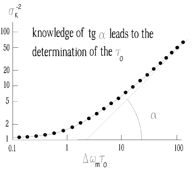
Figure 6: Typical behavior of the variance associated with the measurement of the number of photoelectrons per pulse as a function of lifetime and monochromator bandwidth

At the opposite extreme, with a lifetime much longer than the coherence time, the fact that many independent fluctuations of the instantaneous intensity occur within the interval $\tau_{0}$ implies, according to the theory of completely chaotic light, that the variance is inversely proportional to the monochromator bandwidth. So, we obtain the rule that the product of lifetime and monochromator bandwidth is of the order of

$$\Delta\omega_{\mathrm{m}}\tau_{0}\simeq\sigma^{-2}_{\mathrm{K}}\qquad{\mathrm{for}}\quad\Delta\omega_{\mathrm{m}}\tau_{0}\gg 1\ .$$

This relation is illustrated in Fig. 6, which shows the parameter $\sigma^{-2}_{\mathrm{K}}$ plotted against $\Delta\omega_{\mathrm{m}}\tau_{0}$. The exact results can in fact be found for certain monochromator line shapes using the formalism introduced in Section 2. The dependence of $\sigma^{-2}_{\mathrm{K}}$ on the exact shape of the signal and of the monochromator profile is rather weak and can be ignored outside the range $0.1<\Delta\omega_{\mathrm{m}}\tau_{0}<10$.

It is important to note that the photocount fluctuations discussed above originate from the shot noise in the electron beam. Nevertheless, the problem of photocount fluctuations is more complicated and there is another (parasitic) fluctuation effect that can be important for the proposed pump-probe experiments. The problem is the time jitter of electron bunch and pump pulse. Any measurement of photocounts will be accompanied by these unavoidable fluctuations. To solve this problem, femtosecond pump pulses from the laser system should be synchronized to the master clock of the storage ring rf system with phase-locking technique. At present the best achievable synchronization between the optical laser and the synchrotron light source is of the order of a few picoseconds. On the other hand the electron bunch length is about of 100 ps. Assuming that the electron bunch envelope is Gaussian distribution (in practice, this is a good assumption) we can find that the parasitic photocount variance reaches a value of about a per cent only. Thus we find that pump pulse jitter should not be a serious limitation in our case.

The next problem is to define the sensitivity of the proposed pump-probe method. A general study of the noise fluctuations associated with the photoevents would be nontrivial. The difficulty arises in simultaneously including the effects of both the classically induced fluctuations and Poisson noise fluctuations associated with the basic interaction of light and matter. The ratio of the classical variance to the ”photon noise” variance is named as a photocount degeneracy parameter $\delta_{\mathrm{c}}$ (see section 4). Physically speaking, the count degeneracy parameter can be interpreted as the average number of counts that occur in a single coherence interval of the incident (transversely coherent) radiation. It can also be described as the average number of counts per ”degree of freedom” or per ”mode” of the incident wave. When $\delta_{\mathrm{c}}\ll 1$, it is highly probable that there will be no more than one count per coherence interval of the wave, with the result that quantum noise predominates over classically induced noise. On the other hand, when $\delta_{\mathrm{c}}\gg 1$, there are many photoevents presented in each coherence interval of the wave. The result is a ”bunching” of the photoevents by the classical intensity fluctuations, and an increase of the variance of the counts to the point where the classically induced fluctuations are far stronger than the quantum noise variations.

Let us consider the case when the degeneracy parameter is much larger than unity, $\delta_{\mathrm{c}}\gg 1$. The fluctuations of the photoevents are defined mainly by the classical noise in this case and the signal-to-noise ratio for the proposed device can be written in the form

$$\frac{S}{N}=\frac{\sqrt{N_{\mathrm{shot}}}\langle(K-\langle K\rangle)^{2}\rangle}{\sqrt{\langle(K-\langle K\rangle)^{4}\rangle-\langle(K-\langle K\rangle)^{2}\rangle^{2}}}\qquad{\mathrm{for}}\qquad\delta_{\mathrm{c}}\gg 1\ ,$$ (1)

where $N_{\mathrm{shot}}$ is the number of independent measurements averaged in the accumulator (total number of shots). The determination of the signal-to-noise ratio is a nontrivial problem. Fortunately, in the particular case, namely, $\tau_{\mathrm{c}}\gg\tau_{0}$, a much simplified analysis is sufficient. In this case the expression (1) can be reduced to

$$S/N\simeq\sqrt{N_{\mathrm{shot}}/8}\qquad{\mathrm{for}}\qquad\delta_{\mathrm{c}}\gg 1\ ,\quad\Delta\omega_{\mathrm{m}}\tau_{0}\ll 1\ .$$

The signal-to-noise ratio depends on the degeneracy parameter when $\delta_{\mathrm{c}}$ is much less than unity. In this case one can derive that

$$S/N\simeq\delta^{3/2}_{\mathrm{c}}\sqrt{N_{\mathrm{shot}}}\qquad{\mathrm{for}}\qquad\delta_{\mathrm{c}}\ll 1\ ,\quad\Delta\omega_{\mathrm{m}}\tau_{0}\ll 1\ .$$

The significance of the result we have obtained cannot be fully appreciated until we determine typical values of the degeneracy parameter that can be expected in practice. Let us consider the case of radiation with a sufficiently long coherence time that $\tau_{\mathrm{c}}\gg\tau_{0}$. Under such condition, the photocount degeneracy parameter can be estimated simply as (see section 5)

$$\delta_{\mathrm{c}}\simeq\eta(\Delta\omega_{\mathrm{m}}\tau_{0})\left(R_{\mathrm{m}}\frac{\lambda^{3}B_{\mathrm{peak}}}{4c}\right)\qquad{\mathrm{for}}\qquad\Delta\omega_{\mathrm{m}}\tau_{0}\ll 1\ ,$$ (2)

where $\eta$ is the quantum efficiency of photoelectron production, $R_{\mathrm{m}}$ is the monochromator throughput, $\lambda$ is the radiation wavelength, $B_{\mathrm{peak}}$ is the peak spectral brightness. Our physical interpretation of the result (2) is as follows. In order to use the radiation from the undulator it first has to be spatially filtered and monochromatized (see Fig. 4). We interpret the factor $R_{\mathrm{m}}\lambda^{3}B_{\mathrm{peak}}/(4c)$ as representing the number of photons per coherence interval at the monochromator exit, whereas the factor $\Delta\omega_{\mathrm{m}}\tau_{0}$ represents a ratio of integration time $\tau_{0}$ to coherence interval $\tau_{\mathrm{c}}\simeq 1/\Delta\omega_{\mathrm{m}}$. Let us present a specific numerical example for the case of a third-generation synchrotron light source. The spectral brightness delivered by an undulators at a wavelength of $\lambda\simeq 10$ nm is about $B_{\mathrm{peak}}\simeq 10^{21}$ photons/s/0.1%BW/${\mathrm{mm}}^{2}/{\mathrm{mrad}}^{2}$ and the degeneracy parameter is about $\delta_{\mathrm{c}}\simeq 10^{3}\eta R_{\mathrm{m}}$ for the case when $\tau_{\mathrm{c}}\simeq\tau_{0}$.

As we mentioned above, the dependence of $\sigma^{-2}_{\mathrm{K}}(\tau_{\mathrm{c}})$ on the exact shape of the signal is rather weak. As a result, the behaviour of the variance as a function of synchrotron radiation coherence time provides only very little information on the sample dynamics. Nevertheless, the described pump-probe technique can be used to quote a ”characteristic time” of the sample dynamics. The typical procedure is to assume a signal shape (generally exponential shape), and to ”determine” the relaxation time $\tau_{0}$ from the known ratio between the $\tau_{0}/\tau_{\mathrm{c}}$ and $\sigma_{\mathrm{K}}^{2}$.

A more complex instrument can be used to characterize the shape of the signal function. The pump-probe technique based on a correlation principle we are describe in section 7 is to use two spatially separated samples and record correlation of the count fluctuations for each value of the delay $\tau$ between two pump laser pulses. Averaged (shot to shot) count product contains information about the shape of the signal function. Another advantage of the correlator measurement is the possibility to remove the monochromator between spatial filter and sample and thus to increase the count degeneracy parameter.

3 Statistical properties of synchrotron radiation

The present section considers the statistical properties of the intensity fluctuations in synchrotron light. In order to give the subject a semblance of continuity, it will be desirable to introduce considerable matter which will be found in any of standard works on statistical optics. Much of the credit for stimulating modern development in statistical analysis of synchrotron radiation is due to Professor’s Goodman book [4], which laid the groundwork for the principles of pump-probe techniques based on statistical properties of synchrotron light. Quite basic similarities between the methods described here and the methods introduced into X-ray free electron laser physics by authors in [5] should be recognized. We here consider the classical theory of the fluctuation experiment, reserving the quantum discussion for section 4, where the theory of intensity fluctuations is reconsidered in terms of the quantized radiation field.

3.1 Shot noise in the electron beam

In this subsection we study the statistical properties of the shot noise in the electron beam. It should be noted that the process under study is nonstationary with finite pulse duration, so in what follows the averaging symbol $\langle\cdots\rangle$ means the ensemble average over bunches.

Let us consider the microscopic picture of the electron beam current at the entrance of the undulator. The electron beam current is made up of moving electrons randomly arriving at the entrance to the undulator:

$$J(t)=(-e)\sum^{N}_{k=1}\delta(t-t_{k})\ ,$$

where $\delta(\cdots)$ is the delta function, $(-e)$ is the charge of the electron, $N$ is the number of electrons in a bunch, and $t_{k}$ is the random arrival time of the electron at the undulator entrance. The electron bunch profile is described by the profile function $F(t)$. The beam current averaged over an ensemble of bunches can be written in the form:

$$\langle J(t)\rangle=(-e)NF(t)\ .$$

For instance for an electron beam with Gaussian distribution of the current along the beam, the profile function is:

$$F(t)=\frac{1}{\sqrt{2\pi}\sigma_{\mathrm{T}}}\exp\left(-\frac{t^{2}}{2\sigma^{2}_{\mathrm{T}}}\right)\ .$$

The probability of arrival of an electron during the time interval $(t,t+\mathop{\mathrm{d}}t)$ is equal to $F(t)\mathop{\mathrm{d}}t$.

The electron beam current, $J(t)$, and its Fourier transform, $\bar{J}(\omega)$, are connected by

$$\bar{J}(\omega)=\int\limits^{\infty}_{-\infty}e^{\mathop{\mathrm{i}}\omega t}J(t)\mathop{\mathrm{d}}t=(-e)\sum^{N}_{k=1}e^{\mathop{\mathrm{i}}\omega t_{k}}\ ,$$ (3)

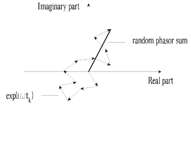
Figure 7: Diagram to show the amplitude and phase of the resultant vector (total complex amplitude) formed by a large number of unit vectors (elementary complex-valued contributions $\exp(\mathop{\mathrm{i}}\omega t_{k})$), each of which has a randomly chosen phase angle

$$J(t)=\frac{1}{2\pi}\int\limits^{\infty}_{-\infty}\bar{J}(\omega)e^{-\mathop{\mathrm{i}}\omega t}\mathop{\mathrm{d}}\omega=(-e)\sum^{N}_{k=1}\delta(t-t_{k})\ .$$

It follows from these expressions that the Fourier transform of the input current, $\bar{J}(\omega)$, is the sum of a large number of complex phasors with random phases $\phi_{k}=\omega t_{k}$. When the electron pulse duration, $\sigma_{\mathrm{T}}$, is long, $\omega\sigma_{\mathrm{T}}\gg 1$, the phases $\phi_{k}$ can be regarded as uniformly distributed on the interval $(0,2\pi)$. The formal summation of the phasors is illustrated in Fig. 7. The calculation is an example of the ”random walk” problem, well known in the theory of stochastic process. In this case we can use the central limit theorem and conclude that the real part and the imaginary part of $\bar{J}(\omega)$ are distributed in accordance with the Gaussian law [4]. The probability density distribution of $\mid\bar{J}(\omega)\mid^{2}$ is given by the negative exponential distribution:

$$p(\mid\bar{J}(\omega)\mid^{2})=\frac{1}{\langle\mid\bar{J}(\omega)\mid^{2}\rangle}\exp\left(-\frac{\mid\bar{J}(\omega)\mid^{2}}{\langle\mid\bar{J}(\omega)\mid^{2}\rangle}\right)\ .$$ (4)

3.2 First-order spectral correlation

Let us calculate the first-order correlation of the complex Fourier harmonics $\bar{J}(\omega)$ and $\bar{J}(\omega^{\prime})$:

$$\langle\bar{J}(\omega)\bar{J}^{*}(\omega^{\prime})\rangle=e^{2}\langle\sum^{N}_{k=1}\sum^{N}_{n=1}\exp(\mathop{\mathrm{i}}\omega t_{k}-\mathop{\mathrm{i}}\omega^{\prime}t_{n})\rangle\ .$$

Expanding this relation, we can write:

$$\langle\bar{J}(\omega)\bar{J}^{*}(\omega^{\prime})\rangle=e^{2}\langle\sum^{N}_{k=1}\exp[\mathop{\mathrm{i}}(\omega-\omega^{\prime})t_{k}]\rangle+e^{2}\sum_{k\neq n}\langle\exp(\mathop{\mathrm{i}}\omega t_{k})\rangle\langle\exp(-\mathop{\mathrm{i}}\omega^{\prime}t_{n})\rangle\ .$$

Expression $\langle\exp(\mathop{\mathrm{i}}\omega t_{k})\rangle$ is equal to the Fourier transformation of the bunch profile function $F(t)$:

$$\langle\exp(\mathop{\mathrm{i}}\omega t_{k})\rangle=\int\limits^{\infty}_{-\infty}F(t_{k})e^{\mathop{\mathrm{i}}\omega t_{k}}\mathop{\mathrm{d}}t_{k}=\bar{F}(\omega)\ .$$

Thus we can write:

$$\langle\bar{J}(\omega)\bar{J}^{*}(\omega^{\prime})\rangle=e^{2}N\bar{F}(\omega-\omega^{\prime})+e^{2}N(N-1)\bar{F}(\omega)\bar{F}(\omega^{\prime})\ .$$

When

$$N\mid\bar{F}(\omega)\mid^{2}\ll 1\ ,$$ (5)

we can write the following expression for the first-order spectral correlation:

$$\langle\bar{J}(\omega)\bar{J}^{*}(\omega^{\prime})\rangle=e^{2}N\bar{F}(\omega-\omega^{\prime})\ .$$ (6)

The Fourier transform of the Gaussian profile function has the form:

$$\bar{F}(\omega)=\exp\left(-\frac{\omega^{2}\sigma_{\mathrm{T}}^{2}}{2}\right)\ .$$

For the specific cases of a Gaussian profile of the electron bunch, the first-order correlation of the complex Fourier harmonics, $\bar{J}(\omega)$ and $\bar{J}(\omega^{\prime})$, has the form:

$$\langle\bar{J}(\omega)\bar{J}^{*}(\omega^{\prime})\rangle=e^{2}N\exp\left[-\frac{(\omega-\omega^{\prime})^{2}\sigma^{2}_{\mathrm{T}}}{2}\right]\ .$$ (7)

Let us discuss the region of validity of the approximation (5). The physical meaning of (5) is that the frequency $\omega$ has to be large enough, $\omega\sigma_{\mathrm{T}}\gg 1$. To be specific, we consider a numerical example for a Gaussian bunch profile. The value of $\mid\bar{F}(\omega)\mid^{2}$ is equal to $\exp(-10^{12})$ when $\sigma_{\mathrm{T}}\omega=10^{6}$. So condition (5) is always fulfilled in practice.

3.3 Second-order spectral correlation

Let us calculate the second order correlation of the complex Fourier harmonics $\bar{J}(\omega)$ and $\bar{J}(\omega^{\prime})$:

$$\langle\mid\bar{J}(\omega)\mid^{2}\mid\bar{J}(\omega^{\prime})\mid^{2}\rangle=e^{4}\langle\sum^{N}_{n=1}\sum^{N}_{m=1}\sum^{N}_{p=1}\sum^{N}_{q=1}\exp[\mathop{\mathrm{i}}\omega(t_{n}-t_{m})+\mathop{\mathrm{i}}\omega^{\prime}(t_{p}-t_{q})]\rangle\ .$$

The $N^{4}$ terms in this sum can be set in 15 classes [4]. When condition (5) is fulfilled, only two of them are of importance, corresponding to $(n=m,\quad p=q,\quad n\neq p)$ and $(n=q,\quad m=p,\quad n\neq m)$. Thus we can write:

$$\langle\mid\bar{J}(\omega)\mid^{2}\mid\bar{J}(\omega^{\prime})\mid^{2}\rangle=\langle\mid\bar{J}(\omega)\mid^{2}\rangle\langle\mid\bar{J}(\omega^{\prime})\mid^{2}\rangle+\mid\langle\bar{J}(\omega)\bar{J}(\omega^{\prime})\rangle\mid^{2}\ .$$ (8)

Substituting (7) into (8) we obtain:

$$\langle\mid\bar{J}(\omega)\mid^{2}\mid\bar{J}(\omega^{\prime})\mid^{2}\rangle=e^{4}N^{2}(1+\mid\bar{F}(\omega-\omega^{\prime})\mid^{2})\ .$$ (9)

3.4 The origin of shot noise in the electron beam

Why is it that the noise in electron beam is a Gaussian random process? Why is this the right rule, what is the fundamental reason for it, and how is it connected to anything else? The explanation is deep down in quantum mechanics. It is generally accepted that quantum mechanics provides the best current picture of physical phenomena, and the most complete description of the radiation field must be sought in quantum-mechanical terms. The quantum theory of radiation predicts the existence of zero-point electromagnetic field. The first step is to show that a field mode is equivalent to harmonic oscillator. To describe a field mode quantum mechanically, we simply describe the equivalent harmonic oscillator quantum mechanically. The vacuum state $\mid 0\rangle$ has no photons, but predicts that it nevertheless has an energy $\hbar\omega/2$. From the probability distribution for a ground-state harmonic oscillator, we easily obtain the probability distribution for the electric field in vacuum state $\mid 0\rangle$. What is the physical significance of these vacuum-state expectation values? One thing they indicate is that the electromagnetic vacuum is a stationary state of the field with statistical fluctuations of the electric and magnetic fields. As far as measurements are concerned, however, it is often argued that the entire universe is evidently bathed in zero-point electromagnetic field, which is distributed according to a Gaussian probability distribution [6].

Relativistic electron beam passing through bending magnets emits synchrotron radiation, a process that leads to damping. In standard classical electrodynamics there is only the radiation reaction field to act on a single particle in the vacuum. All six degrees of freedom for electron motion in storage ring are damped and the actual value of electron beam emittance would be equal to zero. We deduce the synchrotron radiation formula using a classical treatment. So, the reasonable question arises of whether such a classical model describes correctly the synchrotron radiation in the storage ring. Simple physical considerations show that such a description is valid for any practical situation. The classical electrodynamics approach can be used when the energy of the radiated photon $\hbar\omega$ is much less than the energy of the electron. As a rule , $\hbar\omega/(mc^{2}\gamma)\simeq 10^{-5}$ and quantum effects are negligible. Classically we generally assume implicitly that the homogeneous solution of the Maxwell equations is that in which the electric and magnetic fields vanish identically. That is, we assume that there are no fields in the absence of any sources. In the absence of sources the vacuum field is simply zero, with no energy or fluctuations whatsoever. This is not to say that we cannot have source-free fields in classical electrodynamics. Rather, the absence of zero-point fields in standard classical theory lies in the assumption that there are no fields in the absence of any sources.

We can go beyond standard classical theory and postulate the existence of zero-point electric and magnetic fields in the absence of any sources. The difference between classical and quantum electrodynamics, together with the evident importance of the fluctuating vacuum field in quantum electrodynamics, suggests the adoption of a different boundary conditions in classical electrodynamics: instead of assuming that the classical field vanishes in the absence of sources, we can assume that there is a fluctuating classical field with zero energy $\hbar\omega/2$ per mode. As long as this field satisfies the Maxwell’s equations there is no a priori inconsistency in this assumption. The appearance of $\hbar$ in this modification of classical electrodynamics implies no deviation from conventional classical ideas, for $\hbar$ is regarded as nothing more than a number chosen to obtain consistency of the predictions of the theory with experiment. The resulting theory is able to account quantum effects within a fully classical framework [6].

We note that electron storage rings have provided strong evidence for the reality of zero-point energy. In the experiments with stored electrons the zero-point energy sets a lower limit to freezing of the electron motion. If there were no noise associated with the vacuum fields, the actual value of electron beam emittance would be equal to zero. In storage rings damping will counteract quantum excitation leading to an equilibrium. If one looks over the derivation of the quantum diffusion of the electrons in the storage ring, it becomes clear that the argument can be couched in the language of stochastic electrodynamics rather than quantum electrodynamics. That is , all that is really required in that derivation is zero-point energy $\hbar\omega/2$ per mode of the electromagnetic field. Whether this zero-point energy is of quantum or classical origin is irrelevant for the purpose of deriving the diffusion coefficient - stochastic electrodynamics accounts perfectly well for the quantum diffusion of electrons in storage ring. In this case both the field and the particles are treated classically and we have no practical need in accelerator physics for quantum electrodynamics.

The diffusion terms will introduce a statistical mixing of the phases and after some damping times any initial azimuthal variation of the phase space density will be washed out. Electrons in a storage ring are evidently bathed in zero-point electromagnetic field, which is distributed according to a Gaussian probability distribution. This is the explanation of the relation between vacuum fluctuations and shot noise in the electron beam.

3.5 Analysis of synchrotron radiation properties in the frequency domain

Above we described the properties of the input shot noise signal in the frequency domain. The next step is the derivation of the spectral function connecting the Fourier amplitudes of the output field and the Fourier amplitudes of the input noise signal. In the first analysis of the problem, we adopt some rather simplifying assumptions that are only occasionally met in practice. Following this simplified analysis, however, we show how the validity of the results can be extended to a far wider range of conditions than might have been thought at the start.

We will investigate the synchrotron radiation in the framework of the one-dimensional model. For simplicity we consider linear polarization of synchrotron radiation, and use a scalar representation of the radiation field. Nevertheless, all the results are valid for any polarization. The one-dimensional model describes the radiation of the plane electromagnetic wave

$$E_{y}(t)=\tilde{E}_{y}(t)\exp[\mathop{\mathrm{i}}\omega(z/c-t)]+{\mathrm{C.C.}}\ ,$$

by the electron beam in the planar undulator. The electric field of the electromagnetic wave in the time domain, $E_{y}(t)$, and its Fourier transform, $\bar{E}(\omega)$, are connected by

$$E_{y}(t)=\frac{1}{2\pi}\int\limits^{\infty}_{-\infty}\bar{E}(\omega)e^{-\mathop{\mathrm{i}}\omega t}\mathop{\mathrm{d}}\omega\ .$$

When $\omega<0$ the Fourier harmonic is defined by the relation $\bar{E}^{*}(\omega)=\bar{E}(-\omega)$. The Fourier harmonic of the transversely coherent electromagnetic field at the spatial filter exit and the Fourier harmonic of the current at the undulator entrance are connected by the relation:

$$\bar{E}(\omega)=A(\omega)\bar{J}(\omega)\ ,\quad\omega>0\ ,$$ (10)

where $A(\omega)$ is the spectral function of the undulator. For an undulator of $N_{\mathrm{w}}$ periods each electron oscillates through $N_{\mathrm{w}}$ cycles of its motion and thus radiates a wavetrain consisting of $N_{\mathrm{w}}$ cycles of the electric field. The Fourier transform of this waveform which gives the spectral content of the fields, is $\sin(x)/x$, where $x=N_{\mathrm{w}}\pi(\Delta\omega/\omega_{0})$ and $\Delta\omega=(\omega-\omega_{0})$ is the frequency shift away from the central maximum at $\omega_{0}$. Thus we can write (see section 4):

$$\mid A(\omega)\mid^{2}=A_{0}\frac{\sin^{2}(N_{\mathrm{w}}\pi\Delta\omega/\omega_{0})}{(N_{\mathrm{w}}\pi\Delta\omega/\omega_{0})^{2}}\ .$$

It is relevant to make some remarks on the region of applicability of the one-dimensional theory. One-dimensional model assumes the input shot noise and output radiation to have full transverse coherence. This assumption allow us to assume that the input shot noise signal is defined by the value of beam current (10). In reality the fluctuations of the electron beam current density are uncorrelated in the transverse dimension. Using the notion of the beam radiation modes, we can say that many transverse radiation modes are radiated when the electron beam enters the undulator. The one-dimensional model can be used for the calculations of statistical properties of transversely coherent synchrotron radiation. In practice such an assumption is valid for synchrotron light at the exit of a spatial filter. During the spatial filtering process, the number of transverse modes decreases, and the contribution of the coherent radiation into the total radiation power is increased up to full coherence. With this assumption, attention can be concentrated completely on temporal coherence effects.

Here we have used the simplest model of synchrotron light source with zero energy spread into electron beam. In addition, it is assumed that the electrons move along constrained sinusoidal trajectories in parallel with the undulator axis. The first assumption is primarily a statement that the energy spread, $\Delta\gamma/\gamma$, is so small that $N_{\mathrm{w}}\Delta\gamma/\gamma\ll 1$. Such a condition is generally valid in practice. The second assumption is not generally valid in practice, but it will be removed in section 5.

Above we studied the properties of the Fourier harmonics of the shot noise in the frequency domain. The Fourier harmonics of the output radiation field are connected with the Fourier harmonics of the input shot noise by (10). It follows from (10) that statistical properties of the Fourier amplitudes $\bar{E}(\omega)$ are defined by the statistical properties of the Fourier amplitudes of the input current $\bar{J}(\omega)$. In particular, it follows immediately from (4) that $\mid\bar{E}(\omega)\mid^{2}$ is distributed in accordance with the negative exponential probability density function:

$$p(\mid\bar{E}(\omega)\mid^{2})=\frac{1}{\langle\mid\bar{E}(\omega)\mid^{2}\rangle}\exp\left(-\frac{\mid\bar{E}(\omega)\mid^{2}}{\langle\mid\bar{E}(\omega)\mid^{2}\rangle}\right)\ .$$ (11)

For many practical applications of the synchrotron radiation a monochromator has to be installed at the undulator exit. We denote the frequency profile function of the monochromator as $G_{\mathrm{m}}(\omega)$. The linearity of Maxwell’s equations and the fact that a monochromator can be treated as a linear filter allows one to write the Fourier components of the electric field of the synchrotron radiation in the following form:

$$\bar{E}(\omega)=A(\omega)G_{\mathrm{m}}(\omega)\bar{J}(\omega)\ ,\qquad\omega>0\ ,$$ (12)

Let us calculate the correlation of the complex Fourier harmonics $\bar{E}(\omega)$ and $\bar{E}(\omega^{\prime})$. When the monochromator bandwidth is much less than the spectral bandwidth of the undulator radiation we obtain:

$$\langle\bar{E}(\omega)\bar{E}^{*}(\omega^{\prime})\rangle=\mid A(\omega_{0})\mid^{2}G_{\mathrm{m}}(\omega-\omega_{0})G_{\mathrm{m}}^{*}(\omega^{\prime}-\omega_{0})\langle\bar{J}(\omega)\bar{J}^{*}(\omega^{\prime})\rangle\ .$$ (13)

It is seen from (6) that one can write (13) as

$$\langle\bar{E}(\omega)\bar{E}^{*}(\omega^{\prime})\rangle=e^{2}N\mid A(\omega_{0})\mid^{2}G_{\mathrm{m}}(\omega-\omega_{0})G_{\mathrm{m}}^{*}(\omega^{\prime}-\omega_{0})\bar{F}(\omega-\omega^{\prime})\ .$$ (14)

The first-order spectral correlation function is defined as

$$g_{1}(\omega-\omega^{\prime})=\frac{\langle\bar{E}(\omega)\bar{E}^{*}(\omega^{\prime})\rangle}{\sqrt{\langle\mid\bar{E}(\omega)\mid^{2}\rangle\langle\mid\bar{E}(\omega^{\prime})\mid^{2}\rangle}}\ .$$ (15)

Substituting (14) into (15), we obtain

$$\mid g_{1}(\omega-\omega^{\prime})\mid=\mid\bar{F}(\omega-\omega^{\prime})\mid\ .$$ (16)

The explicit expression for the first-order spectral correlation function of the synchrotron radiation emitted by the electron bunch with Gaussian profile has the form:

$$g_{1}(\omega-\omega^{\prime})=\exp\left[-\frac{(\omega-\omega^{\prime})^{2}\sigma_{\mathrm{T}}^{2}}{2}\right]\ .$$ (17)

We define the interval of spectral coherence as

$$\Delta\omega_{\mathrm{c}}=\int\limits^{\infty}_{-\infty}\mid g_{1}(\Delta\omega)\mid^{2}\mathop{\mathrm{d}}(\Delta\omega)\ .$$ (18)

The value of the spectral coherence for the synchrotron source with a Gaussian electron bunch is given by

$$\Delta\omega_{\mathrm{c}}=\int\limits^{\infty}_{-\infty}\mid\bar{F}(\Delta\omega)\mid^{2}\mathop{\mathrm{d}}(\Delta\omega)=\frac{\sqrt{\pi}}{\sigma_{\mathrm{T}}}\ .$$ (19)

The second-order spectral correlation function is defined as

$$g_{2}(\omega-\omega^{\prime})=\frac{\langle\mid\bar{E}(\omega)\mid^{2}\mid\bar{E}(\omega^{\prime})\mid^{2}\rangle}{\langle\mid\bar{E}(\omega)\mid^{2}\rangle\langle\mid\bar{E}(\omega^{\prime})\mid^{2}\rangle}\ .$$ (20)

Using (9), (12) and (20) we obtain that the first and second order correlation functions are connected by the relation:

$$g_{2}(\omega-\omega^{\prime})=1+\mid g_{1}(\omega-\omega^{\prime})\mid^{2}\ ,$$ (21)

which is also a general property of completely chaotic polarized radiation. The explicit expression for the second-order spectral correlation function for the synchrotron source with Gaussian electron bunch has the form:

$$g_{2}(\omega-\omega^{\prime})=1+\mid\bar{F}(\omega-\omega^{\prime})\mid^{2}=1+\exp\left[-(\omega-\omega^{\prime})^{2}\sigma_{\mathrm{T}}^{2}\right]\ .$$

3.6 Energy fluctuation experiment

In this subsection we are going to discuss the application of statistical optics to a practical device. We will find that many of the features of this specific problem are quite common in the general statistical theory of synchrotron light, and we will learn a great deal by considering this one problem in detail.

Figure 8 shows the fluctuation experiment geometry under consideration. The problem is a description of the fluctuations of the energy of the radiation pulse $W$ at the detector installed after the spatial filter and monochromator. The experiment is here analyzed in some detail to determine the conditions under which the field fluctuations, resulting from the chaotic nature of the light source, affect the energy fluctuations. Note that in this experiment, both monochromator resolution and radiation pulse duration play a role. There is no X-ray monochromator providing the coherence time $\tau_{\mathrm{c}}\simeq\lambda^{2}/c\Delta\lambda$ comparable with radiation pulse duration (100 ps). The model experiment ignores these technical limitations.

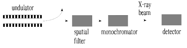
Figure 8: Set-up of model experiment

Using the expression for Poynting’s vector and Parseval’s theorem, we calculate the radiation energy in one radiation pulse:

$$W=\frac{cS}{4\pi}\int\limits^{\infty}_{-\infty}E_{y}^{2}(t)\mathop{\mathrm{d}}t=\frac{cS}{4\pi^{2}}\int\limits^{\infty}_{0}\mid\bar{E}(\omega)\mid^{2}\mathop{\mathrm{d}}\omega\ ,$$

where $S$ is the transverse area of the detector. The energy, averaged over an ensemble, is given by the expression:

$$\langle W\rangle=\frac{cS}{4\pi^{2}}\int\limits^{\infty}_{0}\langle\mid\bar{E}(\omega)\mid^{2}\rangle\mathop{\mathrm{d}}\omega\ ,$$ (22)

where $\langle\mid\bar{E}(\omega)\mid^{2}\rangle$ is calculated using (6) and (13):

$$\langle\mid\bar{E}(\omega)\mid^{2}\rangle=\mid A(\omega)\mid^{2}\mid G_{\mathrm{m}}(\omega)\mid^{2}\langle\mid\bar{I}(\omega)\mid^{2}\rangle=e^{2}N\mid A(\omega)\mid^{2}\mid G_{\mathrm{m}}(\omega)\mid^{2}\ .$$ (23)

Using (22) and (23), we calculate the average energy measured after the monochromator:

$$\langle W\rangle=\frac{cS}{4\pi^{2}}\int\limits^{\infty}_{0}\langle\mid\bar{E}(\omega)\mid^{2}\rangle\mathop{\mathrm{d}}\omega=\frac{ce^{2}SN}{4\pi^{2}}\int\limits^{\infty}_{0}\mid A(\omega)\mid^{2}\mid G_{\mathrm{m}}(\omega)\mid^{2}\d\omega\ .$$

It is seen that the average energy is a function of the frequency profile of the monochromator and undulator.

The variance of the energy distribution is calculated as follows:

$$\sigma^{2}_{\mathrm{W}}=\frac{\langle(W-\langle W\rangle)^{2}\rangle}{\langle W\rangle^{2}}=\frac{\int\limits^{\infty}_{0}\mathop{\mathrm{d}}\omega\int\limits^{\infty}_{0}\mathop{\mathrm{d}}\omega^{\prime}\langle\mid\bar{E}(\omega)\mid^{2}\mid\bar{E}(\omega^{\prime})\mid^{2}\rangle}{\int\limits^{\infty}_{0}\mathop{\mathrm{d}}\omega\langle\mid\bar{E}(\omega)\mid^{2}\rangle\int\limits^{\infty}_{0}\mathop{\mathrm{d}}\omega^{\prime}\langle\mid\bar{E}(\omega^{\prime})\mid^{2}\rangle}-1\ .$$

Using definition (20) of the second-order correlation function and (21), we reduce this expression to

$$\sigma^{2}_{\mathrm{W}}=\frac{\int\limits^{\infty}_{0}\mathop{\mathrm{d}}\omega\int\limits^{\infty}_{0}\mathop{\mathrm{d}}\omega^{\prime}\langle\mid\bar{E}(\omega)\mid^{2}\rangle\langle\mid\bar{E}(\omega^{\prime})\mid^{2}\rangle\mid g_{1}(\omega-\omega^{\prime})\mid^{2}}{\int\limits^{\infty}_{0}\mathop{\mathrm{d}}\omega\langle\mid\bar{E}(\omega)\mid^{2}\rangle\int\limits^{\infty}_{0}\mathop{\mathrm{d}}\omega^{\prime}\langle\mid\bar{E}(\omega^{\prime})\mid^{2}\rangle}\ .$$ (24)

The analysis of this expression shows that the variance of the energy distribution after the monochromator is a function of the frequency profile of the monochromator, of the frequency profile of the undulator, and of the electron bunch formfactor $\bar{F}(\omega-\omega^{\prime})$.

Let us consider the case of an electron bunch with a Gaussian profile and a monochromator with a rectangular line:

$$\mid G_{\mathrm{m}}(\omega-\omega_{0})\mid^{2}=1\qquad{\mathrm{for}}\qquad\mid\omega-\omega_{0}\mid<\frac{\Delta\omega_{\mathrm{m}}}{2}\ ,$$

$$\mid G_{\mathrm{m}}(\omega-\omega_{0})\mid^{2}=0\qquad{\mathrm{for}}\qquad\mid\omega-\omega_{0}\mid>\frac{\Delta\omega_{\mathrm{m}}}{2}\ .$$

For simplicity we assume that the bandwidth of the monochromator is small and $A(\omega)$ is constant within the monochromator bandwidth. Then the integration of the expression (24) provides the following result:

$$\sigma^{2}_{\mathrm{W}}=\frac{\Delta\omega_{\mathrm{c}}}{\Delta\omega_{\mathrm{m}}}{\mathrm{erf}}\left(\frac{\sqrt{\pi}\Delta\omega_{\mathrm{m}}}{\Delta\omega_{\mathrm{c}}}\right)-\frac{1}{\pi}\left(\frac{\Delta\omega_{\mathrm{c}}}{\Delta\omega_{\mathrm{m}}}\right)^{2}\left\{1-\exp\left[-\pi\left(\frac{\Delta\omega_{\mathrm{m}}}{\Delta\omega_{\mathrm{c}}}\right)^{2}\right]\right\}\ ,$$ (25)

where ${\mathrm{erf}}(x)$ is the error function and $\Delta\omega_{\mathrm{c}}$ is given by expression (19).

Let us study the asymptotic behavior of (25). When the monochromator bandwidth is much less than the interval of spectral coherence, the normalized dispersion tends to unity:

$$\sigma^{2}_{\mathrm{W}}\simeq 1\qquad{\mathrm{for}}\qquad\Delta\omega_{\mathrm{m}}\ll\Delta\omega_{\mathrm{c}}\ .$$

When the monochromator bandwidth is much larger than the interval of spectral coherence, the variance is inversely proportional to the monochromator bandwidth:

$$\sigma^{2}_{\mathrm{W}}\simeq\frac{\Delta\omega_{\mathrm{c}}}{\Delta\omega_{\mathrm{m}}}\qquad{\mathrm{for}}\qquad\Delta\omega_{\mathrm{c}}\ll\Delta\omega_{\mathrm{m}}\ .$$

The next practical problem is to find the probability density distribution of the radiation energy after the monochromator, $p(W)$. Using the well-known results obtained in the framework of statistical optics, we can state that the distribution of the radiation energy after the monochromator is described rather well by the gamma probability density function:

$$p(W)=\frac{M^{M}}{\Gamma(M)}\left(\frac{W}{\langle{W}\rangle}\right)^{M-1}\frac{1}{\langle{W}\rangle}\exp\left(-M\frac{W}{\langle{W}\rangle}\right)\ ,$$ (26)

where $\Gamma(M)$ is the gamma function of argument $M$, and $1/M=\sigma^{2}_{\mathrm{W}}$. This distribution provides correct values for the mean value of $W$ and for the variance $\sigma^{2}_{\mathrm{W}}$:

$$\int\limits^{\infty}_{0}Wp(W)\mathop{\mathrm{d}}W=\langle W\rangle\ ,\quad\int\limits^{\infty}_{0}\frac{(W-\langle W\rangle)^{2}}{\langle W\rangle^{2}}p(W)\mathop{\mathrm{d}}W=\frac{1}{M}\ .$$

The parameter $M$ can be interpreted as the average number of degrees of freedom (or modes) in the radiation pulse. It follows from (24) that this parameter cannot be less than unity. When $M$ tends to the unity, (26) tends to the negative exponential distribution (11). For large values of $M$ the distribution (26) tends to a Gaussian distribution.

3.7 Analysis of the radiation properties in the time domain

An expression for the electric field of the electromagnetic wave as a function of time $t$ can be obtained using the Fourier transform of (12). It is convenient to isolate explicitly the slowly varying complex amplitude:

$$E_{y}(t)=\tilde{E}(t)e^{-\mathop{\mathrm{i}}\omega_{0}t}+{\mathrm{C.C.}}\ ,$$ (27)

where

$$\tilde{E}(t)e^{-\mathop{\mathrm{i}}\omega_{0}t}=\frac{1}{2\pi}\int\limits^{\infty}_{0}\bar{E}(\omega)e^{-\mathop{\mathrm{i}}\omega t}\mathop{\mathrm{d}}\omega\ .$$

Let us consider the specific case of a Gaussian monochromator line profile

$$\mid G_{\mathrm{m}}(\omega)\mid^{2}=\exp\left[-\frac{(\omega-\omega_{0})^{2}}{2\sigma^{2}_{\mathrm{m}}}\right]$$ (28)

allowing calculations of the complex amplitude $\tilde{E}(t)$ of the electric field at the monochromator exit in the limit of small monochromator bandwidth. In other words, we assume $A(\omega)$ to be constant within the monochromator bandwidth.

Using (10), (3), (28) and (27), we obtain:

$$\tilde{E}(t)=E_{0}\left\{\frac{1}{N}\sum^{N}_{k=1}\exp(\mathop{\mathrm{i}}\omega_{0}t_{k})\exp[-\sigma_{\mathrm{m}}^{2}(t-t_{k})^{2}]\right\}\ .$$ (29)

Since $\sigma_{\mathrm{m}}\ll\omega_{0}$, we can approximately let the amplitude and the phase of each random phasor contributing to the sum in (29) be independent of each other, and the phases be uniformly distributed on the interval $(0,2\pi)$. Thus, the distribution of the instantaneous radiation power density $(\ \propto\ \mid\tilde{E}(t)\mid^{2})$ is the negative exponential distribution:

$$p(\mid\tilde{E}(t)\mid^{2})=\frac{1}{\langle\mid\tilde{E}(t)\mid^{2}\rangle}\exp\left(-\frac{\mid\tilde{E}(t)\mid^{2}}{\langle\mid\tilde{E}(t)\mid^{2}\rangle}\right)\ .$$ (30)

The correlation between the radiation fields at times $t$ and $t^{\prime}$ has the form:

$$\langle\tilde{E}(t)\tilde{E}^{*}(t^{\prime})\rangle\exp[-\mathop{\mathrm{i}}\omega_{0}(t-t^{\prime})]$$

$$=\frac{1}{4\pi^{2}}\int\limits^{\infty}_{0}\mathop{\mathrm{d}}\omega\int\limits^{\infty}_{0}\mathop{\mathrm{d}}\omega^{\prime}\exp(-\mathop{\mathrm{i}}\omega t+\mathop{\mathrm{i}}\omega^{\prime}t^{\prime})\langle\bar{E}(\omega)\bar{E}^{*}(\omega^{\prime})\rangle$$

$$=\frac{1}{4\pi^{2}}\int\limits^{\infty}_{0}\mathop{\mathrm{d}}\omega\int\limits^{\infty}_{0}\mathop{\mathrm{d}}\omega^{\prime}\exp(-\mathop{\mathrm{i}}\omega t+\mathop{\mathrm{i}}\omega^{\prime}t^{\prime})$$

$$\times[\langle\mid\bar{E}(\omega)\mid^{2}\rangle\langle\mid\bar{E}(\omega^{\prime})\mid^{2}\rangle]^{1/2}\bar{F}(\omega-\omega^{\prime})\ .$$ (31)

Here (15) and (16) have been used when rewriting the integral. In the present consideration we use the approximation which assumes the interval of spectral coherence is much less than the monochromator bandwidth

$$\Delta\omega_{\mathrm{c}}\ll\sigma_{\mathrm{m}}\ .$$ (32)

Thus we can simplify the integral in the following way. We replace the expression in square brackets by $\langle\mid\bar{E}(\omega)\mid^{2}\rangle$, and after integration over $\omega$ and $\Delta\omega=(\omega-\omega^{\prime})$ we obtain:

$$\langle\tilde{E}(t)\tilde{E}^{*}(t^{\prime})\rangle\exp[-\mathop{\mathrm{i}}\omega_{0}(t-t^{\prime})]$$

$$=\frac{1}{4\pi^{2}}\int\limits^{\infty}_{0}\mathop{\mathrm{d}}(\Delta\omega)\exp(-\mathop{\mathrm{i}}\Delta\omega t)\bar{F}(\Delta\omega)\int\limits^{\infty}_{0}\mathop{\mathrm{d}}\omega\exp[-\mathop{\mathrm{i}}\omega(t-t^{\prime})]\langle\mid\bar{E}(\omega)\mid^{2}\rangle$$

$$=\frac{F(t)}{2\pi}\int\limits^{\infty}_{0}\mathop{\mathrm{d}}\omega\exp[-\mathop{\mathrm{i}}\omega(t-t^{\prime})]\langle\mid\bar{E}(\omega)\mid^{2}\rangle\ ,$$ (33)

where $F(t)$ is the radiation pulse profile. We define the first-order time correlation function as follows:

$$g_{1}(t-t^{\prime})=\frac{\langle\tilde{E}(t)\tilde{E}^{*}(t^{\prime})\rangle}{\left[\langle\mid\tilde{E}(t)\mid^{2}\rangle\langle\mid\tilde{E}(t^{\prime})\mid^{2}\rangle\right]^{1/2}}\ .$$

Using (33), we can write

$$g_{1}(t-t^{\prime})=\frac{\int\limits^{\infty}_{0}\mathop{\mathrm{d}}\omega\langle\mid\bar{E}(\omega)\mid^{2}\rangle\exp[-\mathop{\mathrm{i}}(\omega-\omega_{0})(t-t^{\prime})]}{\int\limits^{\infty}_{0}\mathop{\mathrm{d}}\omega\langle\mid\bar{E}(\omega)\mid^{2}\rangle}$$

Since we deal with a narrow-band signal, the latter expression may be rewritten as follows

$$g_{1}(t-t^{\prime})=\frac{\int\limits^{\infty}_{-\infty}\mathop{\mathrm{d}}(\Delta\omega)\langle\mid\bar{E}(\Delta\omega)\mid^{2}\rangle\exp[-\mathop{\mathrm{i}}(\Delta\omega)(t-t^{\prime})]}{\int\limits^{\infty}_{-\infty}\mathop{\mathrm{d}}(\Delta\omega)\langle\mid\bar{E}(\Delta\omega)\mid^{2}\rangle}\ ,$$ (34)

where $\Delta\omega=(\omega-\omega_{0})$. Therefore, the slowly varying correlation function and the normalized spectrum of the narrow-band signal are a Fourier transform pair. Remembering relation (10), we rewrite (34) in the following way:

$$g_{1}(t-t^{\prime})=\frac{\int\limits^{\infty}_{-\infty}\mathop{\mathrm{d}}(\Delta\omega)\mid G_{\mathrm{m}}(\Delta\omega)\mid^{2}\exp[-\mathop{\mathrm{i}}(\Delta\omega)(t-t^{\prime})]}{\int\limits^{\infty}_{-\infty}\mathop{\mathrm{d}}(\Delta\omega)\mid G_{\mathrm{m}}(\Delta\omega)\mid^{2}}\ .$$

It is seen from this expression that the first-order correlation function possesses the property $g_{1}(t-t^{\prime})=g_{1}^{*}(t^{\prime}-t)$. When the monochromator line profile is symmetrical the function $g_{1}$ is real. For instance, for a monochromator with Gaussian line profile the correlation function $g_{1}$ is

$$g_{1}(\tau)=\exp\left(-\frac{\sigma^{2}_{\mathrm{m}}\tau^{2}}{2}\right)\ ,$$ (35)

where $\tau=(t-t^{\prime})$. Following the approach of Mandel, we define the coherence time, $\tau_{\mathrm{c}}$, as

$$\tau_{\mathrm{c}}=\int\limits^{\infty}_{-\infty}\mid g_{1}(\tau)\mid^{2}\mathop{\mathrm{d}}\tau\ .$$

For the case of the Gaussian line profile , the explicit expression for the coherence time is

$$\tau_{\mathrm{c}}=\frac{\sqrt{\pi}}{\sigma_{\mathrm{m}}}\ .$$ (36)

The correlation between the radiation intensities at times $t$ and $t^{\prime}$ is defined as

$$\langle\mid\tilde{E}(t)\mid^{2}\mid\tilde{E}(t^{\prime})\mid^{2}\rangle$$

$$=\frac{1}{16\pi^{4}}\int\limits^{\infty}_{0}\mathop{\mathrm{d}}\omega_{1}\int\limits^{\infty}_{0}\mathop{\mathrm{d}}\omega_{2}\int\limits^{\infty}_{0}\mathop{\mathrm{d}}\omega_{3}\int\limits^{\infty}_{0}\mathop{\mathrm{d}}\omega_{4}\exp[-\mathop{\mathrm{i}}(\omega_{1}-\omega_{2})t-\mathop{\mathrm{i}}(\omega_{3}-\omega_{4})t^{\prime})]$$

$$\times\langle\bar{E}(\omega_{1})\bar{E}(\omega_{3})\bar{E}^{*}(\omega_{2})\bar{E}^{*}(\omega_{4})\rangle\ .$$ (37)

Taking into account (12), (3) and (5), we simplify the correlation in the integrand of (37) in the following way:

$$\langle\bar{E}(\omega_{1})\bar{E}(\omega_{3})\bar{E}^{*}(\omega_{2})\bar{E}^{*}(\omega_{4})\rangle$$

$$=\langle\bar{E}(\omega_{1})\bar{E}^{*}(\omega_{2})\rangle\langle\bar{E}(\omega_{3})\bar{E}^{*}(\omega_{4})\rangle$$

$$+\langle\bar{E}(\omega_{1})\bar{E}^{*}(\omega_{4})\rangle\langle\bar{E}(\omega_{3})\bar{E}^{*}(\omega_{2})\rangle\ ,$$ (38)

and present the integral (37) as the sum of two terms. To calculate the integral, one should take into account (15), (16), (33) and (32) , which leads to

$$\langle\mid\tilde{E}(t)\mid^{2}\mid\tilde{E}(t^{\prime})\mid^{2}\rangle=\langle\mid\tilde{E}(t)\mid^{2}\rangle\langle\mid\tilde{E}(t^{\prime})\mid^{2}\rangle+\mid\langle\tilde{E}(t)\tilde{E}^{*}(t^{\prime})\rangle\mid^{2}\ .$$ (39)

The second-order time correlation function is defined as follows:

$$g_{2}(t-t^{\prime})=\frac{\langle\mid\tilde{E}(t)\mid^{2}\mid\tilde{E}(t^{\prime})\mid^{2}\rangle}{\langle\mid\tilde{E}(t)\mid^{2}\rangle\langle\mid\tilde{E}(t^{\prime})\mid^{2}\rangle}\ .$$ (40)

It follows from (39) and definitions of $g_{1}(t-t^{\prime})$ and $g_{2}(t-t^{\prime})$ that

$$g_{2}(t-t^{\prime})=1+\mid g_{1}(t-t^{\prime})\mid^{2}\ .$$ (41)

The analysis of the obtained relations (30) and (41) shows that the synchrotron radiation possesses all the features of completely chaotic polarized light (see also (11) and (21) obtained in the frequency domain).

3.8 Statistical properties of the integrated intensity

In a variety of problems, related with photon-counting statistics, finite-time integrals of instantaneous intensity occur. In many cases the fluctuations in the intensity are too rapid for direct observation, and what is measured is some average of the fluctuations over detector response time. The calculation can be performed without great difficulty in two limiting cases, namely, the response time very long and very short compared with the electron pulse duration. In section 3.6 we discussed in detail fluctuations of the energy of the radiation pulse at the slow detector installed after the monochromator (see Fig. 5). Note that for this class of experiments we actually assume that the integration time is much longer than the electron pulse duration.

Next let us consider the opposite extreme. For our simplified discussion here let us assume that the integration time is much shorter than the electron pulse duration, leaving the electron pulse envelope unaffected. There is no photodetector providing a time resolution much shorter than the X-ray pulse duration. Present-day X-ray detection will be limited in time resolution of about 100 ps. The situation is somewhat different in pump-probe experiments. A pump-probe experiment has analogies with a femtosecond photodetector measurement. The basic analogy is that a femtosecond pump pulse interacts with the sample and excites it into non-equilibrium state. The sample thereafter relaxes towards a new equilibrium state. Typical relaxation times are in the femtosecond range. This process can be mapped by sending a X-ray probe pulse onto the sample. Such a device could be discussed as a femtosecond X-ray detector by recording a secondary process such as photoelectrons.

Several assumptions are made about the profile of the photodetector gating function. For the present, consideration is restricted to the simplest case from the analytical point of view, namely, completely chaotic polarized radiation and an ideal detector with a stepped profile gating function. So, the next problem is the description of the fluctuations of the radiation energy $W$ detected during a finite time interval $\delta T$:

$$W=\int\limits^{t+\delta T}_{t}I(t)\mathop{\mathrm{d}}t\ .$$

The variance is calculated as follows:

$$\sigma^{2}_{\mathrm{W}}=\frac{\langle(W-\langle W\rangle)^{2}\rangle}{\langle W\rangle^{2}}=\frac{1}{(\delta T)^{2}}\int\limits^{t+\delta T}_{t}\mathop{\mathrm{d}}t^{\prime}\int\limits^{t+\delta T}_{t}\mathop{\mathrm{d}}t^{\prime\prime}\frac{\langle I(t^{\prime})I(t^{\prime\prime})\rangle}{\langle I\rangle^{2}}-1$$

$$=\frac{1}{(\delta T)^{2}}\int\limits^{t+\delta T}_{t}\mathop{\mathrm{d}}t^{\prime}\int\limits^{t+\delta T}_{t}\mathop{\mathrm{d}}t^{\prime\prime}\frac{\langle\mid\tilde{E}(t^{\prime})\mid^{2}\mid\tilde{E}(t^{\prime\prime})\mid^{2}\rangle}{\langle\mid\tilde{E}(t^{\prime})\mid^{2}\rangle\langle\mid\tilde{E}(t^{\prime\prime})\mid^{2}\rangle}-1$$

$$=\frac{1}{(\delta T)^{2}}\int\limits^{\delta T}_{0}\mathop{\mathrm{d}}u\int\limits^{\delta T}_{0}\mathop{\mathrm{d}}vg_{2}(u-v)-1\ .$$ (42)

Substituting (40), (41) and (35) into (42) we obtain the following expression for the variance of the energy distribution detected during time interval $\delta T$ for the Gaussian monochromator line profile:

$$\sigma^{2}_{\mathrm{W}}=\frac{1}{(\delta T)^{2}}\int\limits^{\delta T}_{0}\mathop{\mathrm{d}}u\int\limits^{\delta T}_{0}\mathop{\mathrm{d}}v\mid g_{1}(u-v)\mid^{2}$$

$$=\frac{1}{(\delta T)^{2}}\int\limits^{\delta T}_{-\delta T}(\delta T-\tau)\mid g_{1}(\tau)\mid^{2}\mathop{\mathrm{d}}\tau$$

$$=\frac{\sqrt{\pi}}{\delta T\sigma_{\mathrm{m}}}{\mathrm{erf}}(\delta T\sigma_{\mathrm{m}})-\frac{1-\exp[-(\delta T\sigma_{\mathrm{m}})^{2}]}{(\delta T\sigma_{\mathrm{m}})^{2}}\ .$$ (43)

It can be shown that the integrated intensity distribution is described rather well by the gamma probability density function (21) with parameter $M$ equal to $\sigma_{\mathrm{W}}^{-2}$. When $\delta T$ is less than the coherence time $\tau_{\mathrm{c}}$ (36), the parameter $M$ tends to unity and the gamma distribution tends to the negative exponential distribution. In the opposite case, when $\delta T\gg\tau_{\mathrm{c}}$, we can write:

$$M^{-1}=\frac{\sqrt{\pi}}{\delta T\sigma_{\mathrm{m}}}=\frac{\tau_{\mathrm{c}}}{\delta T}\ ,$$

and the gamma distribution tends to a Gaussian distribution.

In some experiments, such as one in which a long probe pulse is being used to measure lifetime of internal conversion of electronic excitation, the photocount time dependence is exponential dependence. In this case the detector gating function is an exponential function and the variance is calculated as follows:

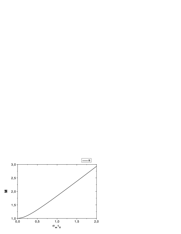
Figure 9: Plot of $M=\sigma^{-2}_{\mathrm{W}}$ versus $\sigma_{\mathrm{m}}\tau_{0}$, exact solution for Gaussian spectral profile and exponential dependence of gating function

$$\sigma^{2}_{\mathrm{W}}=\frac{\int\limits^{\infty}_{0}\mathop{\mathrm{d}}t\int\limits^{\infty}_{0}\mathop{\mathrm{d}}t^{\prime}\exp(-t/\tau_{0})\exp(-t^{\prime}/\tau_{0})\langle\mid\tilde{E}(t)\mid^{2}\mid\tilde{E}(t^{\prime})\mid^{2}\rangle}{\int\limits^{\infty}_{0}\mathop{\mathrm{d}}t\exp(-t/\tau_{0})\langle\mid\tilde{E}(t)\mid^{2}\rangle\int\limits^{\infty}_{0}\mathop{\mathrm{d}}t^{\prime}\exp(-t^{\prime}/\tau_{0})\langle\mid\tilde{E}(t^{\prime})\mid^{2}\rangle}-1\ .$$ (44)

Let the monochromator line profile be Gaussian. Substituting (40), (41) and (35) into (44) we obtain an expression for the variance of the energy distribution:

$$\sigma^{2}_{\mathrm{W}}=\int\limits^{\infty}_{0}\mathop{\mathrm{d}}u\exp(-u)\int\limits^{\infty}_{0}\mathop{\mathrm{d}}v\exp(-v)\exp[-\sigma^{2}_{\mathrm{m}}\tau^{2}_{0}(u-v)^{2}]\ .$$ (45)

There is no simple analytical expression for the variance in this case. In Fig. 9 we present the results of numerical calculations.

Our discussion of integrated intensity fluctuations would be incomplete if we did not refer the reader to another method of calculation. The sample dynamics is in the femtosecond range and $\langle I\rangle={\mathrm{const.}}$ is a good assumption. Clearly, we can assume that the synchrotron light in question is adequately modelled as an ergodic and hence stationary random process. Surely the preferred way to solve the problem of integrated intensity fluctuations must be stationary random process way. Although the origins of the above viewpoint are quite clear and understandable, the conclusions reached regarding the relative merits of stationary and nonstationary analysis are very greatly in error, for several important reasons.

The second method of calculation has the advantage of conceptual simplicity but the disadvantage of being not quite as general as the first method. In defence of our nonstationary analysis we must say that models constructed for nonstationary analysis are inherently more general and flexible. Indeed, they invariably contain the model of a stationary random process as a special case. In the normal course of events, a physicist first encounters statistical optics in an entirely stationary random process framework. In this case correlation functions in the frequency domain are represented by delta functions. The physicists emerging from such an introductory course may feel confident that they have grasped the basic statistical optics concepts and are ready to find a precise answer to almost any problem that comes their way. Nevertheless, there is no difficulty in compiling a long list of examples for which an analysis of nonstationary random processes is required.

The nonstationary random process approach is needed somewhat more complex than the stationary random process approach, for it requires knowledge of the statistical properties of synchrotron radiation not only in the time domain but also in the frequency domain. In the long run, however, the nonstationary random process model is far more powerful and useful than the stationary random process model in solving physical problems of practical interest.

4 Photocount fluctuations in the detector of synchrotron radiation

Almost all devices that measure the intensity of a light beam depend for their operation on the absorption of a portion of the beam, whose energy is converted to a detectable form. The photographic plate, the photomultiplier tube, and ionization and detection of photoelectrons in pump-probe experiments all fall into this category. The present section therefore considers the absorption of light in more detail in order to understand the nature of the intensity measurement process. It is convenient to base the discussion on a practical intensity-measuring device, and we select the photodetector. The photodetector depends for its operation on the photoelectric effect. Since the vast majority of pump-probe detection problems do indeed rest on the photoelectric effect, there is relatively little loss of generality by making this assumption.

Consider a storage ring synchrotron light source. The light from this source falls on the photosurface, and we wish to determine the statistical distribution of the number of photoevents observed in any radiation pulse. Any measurement of light will be accompanied by certain unavoidable fluctuations. We attribute these fluctuations to quantum effects; that is, light can be absorbed only in quanta. We shall deal with the so-called semiclassical theory of photodetection. Such an approach has the benefit of being comparatively simple in terms of the mathematical background required, as well as allowing a greater use of physical intuition. The distinguishing characteristic of this formalism is the fact that electromagnetic fields are treated in a completely classical manner until they interact with the atoms of the photosensitive material on which they are incident. Thus there is no necessity to deal with quantization of the electromagnetic field; only the interaction of the classical field and matter is quantized. Fortunately it has been shown that the predictions of the semiclassical theory are in complete agreement wit the predictions of the more rigorous quantum mechanical approach for all detection problems involving the photoelectric effect [4].

We assume that the radiation reaching the detector has full transverse coherence and that the statistical properties of the radiation follow the laws described in the previous section. It has been shown above that the energy, $W$, in the radiation pulse is unpredictable. Thus, we can predict the probability density $p(W)$ only. In this case the probability of detection of $K$ photons is given by Mandel’s semiclassical formula [4]:

$$P(K)=\int\limits^{\infty}_{0}\frac{(\alpha W)^{K}}{K!}\exp(-\alpha W)P(W)\mathop{\mathrm{d}}W\ ,$$ (46)

where $\alpha=\eta/\hbar\omega_{0}$ and $\eta$ is the quantum efficiency of the photodetector. It should be noted that, when conditioned by knowledge of energy $W$, the number of counts $K$ is a Poisson variable with mean $\alpha W$. Using formula (46) we get the expression for the mean and for the variance of the value of $K$:

$$\langle K\rangle=\alpha\langle W\rangle\ ,\quad\sigma^{2}_{\mathrm{K}}=\frac{\langle K^{2}\rangle-\langle K\rangle^{2}}{\langle K\rangle^{2}}=\frac{1}{\langle K\rangle}+\sigma^{2}_{\mathrm{W}}\ ,$$ (47)

where $\sigma^{2}_{\mathrm{W}}=1/M$ is given by the expression (24). The expression for photocount fluctuations contains two terms. The first term corresponds to the photon ”shot noise” and its origin is in the Poisson distribution. The second term corresponds to the classical fluctuations of the energy in the radiation bunch and takes its origin from the shot noise in the electron bunch. The ratio of the classical variance to the ”photon shot noise” variance is named as a photocount degeneracy parameter $\delta_{\mathrm{c}}$:

$$\delta_{\mathrm{c}}=\frac{\langle K\rangle}{M}\ .$$ (48)

The probability density of the integrated synchrotron radiation intensity, $p(W)$, is the gamma distribution. Substituting (26) into Mandel’s formula (46) and performing integration we come to the negative binomial distribution [4]:

$$P(K)=\frac{\Gamma(K+M)}{\Gamma(K+1)\Gamma(M)}\left(1+\frac{M}{\langle K\rangle}\right)^{-K}\left(1+\frac{\langle K\rangle}{M}\right)^{-M}\ .$$ (49)

When the monochromator has a narrow linewidth, $\Delta\omega_{\mathrm{m}}\tau_{0}\ll 1$, parameter $M$ tends to the unity, and the negative binomial distribution transforms to the Bose distribution:

$$\lim_{M\to 1}P(K)=\frac{\langle K\rangle^{K}}{(1+\langle K\rangle)^{K+1}}\ .$$

The negative binomial distribution tends to the gamma distribution at large values of the count degeneracy parameter $\delta_{\mathrm{c}}$. In particular, the Bose distribution tends to the negative exponential distribution ($\delta_{\mathrm{c}}\simeq\langle K\rangle$ in this case):

$$\lim_{\langle K\rangle\to\infty}\frac{\langle K\rangle^{K}}{(1+\langle K\rangle)^{K+1}}=\frac{1}{\langle K\rangle}\exp\left(-\frac{K}{\langle K\rangle}\right)\ .$$ (50)

In the opposite case, at $\delta_{\mathrm{c}}\to 0$, the negative binomial distribution (49) transforms to the Poisson distribution:

$$\lim_{\delta_{\mathrm{c}}\to 0}P(K)=\frac{\langle K\rangle^{K}}{K!}\exp(-\langle K\rangle)\ .$$

5 Characteristics of undulator radiation

For the proposed concept of time-resolved experiments based on the statistical properties, the critical parameter determining the performance is the count degeneracy parameter, or the average number of photoevents produced in a single coherence interval of the incident radiation. The important role of this parameter is emphasized by giving it a name of its own. Because the count degeneracy parameter is proportional to $\langle K\rangle$, it is also proportional to the quantum efficiency of the photosurface. Sometimes it is useful to remove this dependence on the characteristics of the particular detector that may be present, and to deal with a degeneracy parameter that is a property of the synchrotron light itself. We thus define the wave degeneracy parameter as $\delta_{\mathrm{W}}=\delta_{\mathrm{c}}/\eta$. This new degeneracy parameter may be considered to be the count degeneracy parameter that would be obtained with an ideal detector having a quantum efficiency of unity. The wave degeneracy parameter is simply the average number of photons per mode.

In this section we are particularly concerned about the wave degeneracy parameter. From this section we will see that the degeneracy parameter is $\delta_{\mathrm{W}}\simeq\lambda^{3}B_{\mathrm{peak}}/(4c)$, where $B_{\mathrm{peak}}$ is the peak spectral brightness of the radiation source. Third-generation synchrotron light sources achieve high spectral brightness through very low-emittance electron beams and by inserting into the electron beam a device known as an undulator. The undulator causes the electron beam to undulate or bend back and forth, and this produces very bright and coherent light.

5.1 Number of photons radiated in the central radiation cone

Let us introduce the basic features of undulator radiation. The undulator equation

$$\omega=2ck_{\mathrm{w}}\gamma^{2}\left[1+\frac{K_{\mathrm{w}}^{2}}{2}+\gamma^{2}\theta^{2}\right]^{-1}$$

tells us the frequency of radiation as a function of undulator period $\lambda_{\mathrm{w}}=2\pi k_{\mathrm{w}}$, undulator parameter $K_{\mathrm{w}}$, electron energy $m_{0}c^{2}\gamma$, and polar angle of observation $\theta$. Note that for radiation within the cone of half angle

$$\theta_{\mathrm{cen}}=\frac{\sqrt{1+K_{\mathrm{w}}^{2}/2}}{\gamma\sqrt{N_{\mathrm{w}}}}\ ,$$

the relative spectral FWHM bandwidth is $\Delta\omega/\omega=0.88/N_{\mathrm{w}}$, where $N_{\mathrm{w}}$ is the number of undulator periods. The spectral and angular density of the radiation energy emitted by a single electron during the undulator pass is given by the expression (at zero angle):

$$\frac{\mathop{\mathrm{d}}^{2}{\cal E}}{\mathop{\mathrm{d}}\omega\mathop{\mathrm{d}}\Omega}=\frac{e^{2}N_{\mathrm{w}}\gamma^{2}A^{2}_{\mathrm{JJ}}K_{\mathrm{w}}^{2}}{2c(1+K_{\mathrm{w}}^{2}/2)^{2}}\frac{\sin^{2}[\pi N_{\mathrm{w}}(\omega-\omega_{0})/\omega_{0}]}{[\pi N_{\mathrm{w}}(\omega-\omega_{0})/\omega_{0}]^{2}}\ .$$

Here $\omega_{0}=2\gamma^{2}k_{\mathrm{w}}/(1+K_{\mathrm{w}}^{2}/2)$ is the resonance frequency, $A_{\mathrm{JJ}}=[J_{0}(Q)-J_{1}(Q)]$, where $J_{n}$ is the Bessel function of $n$th order, and $Q=K_{\mathrm{w}}^{2}/(4+2K_{\mathrm{w}}^{2})$. Now we would like to calculate the energy radiated into the central cone. In the small-angle approximation the solid angle is equal to $\mathop{\mathrm{d}}\Omega=\theta\mathop{\mathrm{d}}\theta\mathop{\mathrm{d}}\varphi$. Integration of spectral and angular density over $\omega$ and $\varphi$ gives us factors $\omega_{0}/N_{\mathrm{w}}$ and $2\pi$, respectively. We also have to integrate over $\theta$ from $0$ to $\theta_{\mathrm{cen}}$. Thus, the energy radiated into the central cone by a single electron is given by

$$\Delta{\cal E}_{\mathrm{cen}}\simeq\frac{\pi e^{2}A^{2}_{\mathrm{JJ}}\omega_{0}K_{\mathrm{w}}^{2}}{c(1+K_{\mathrm{w}}^{2}/2)}\ .$$

Individual positions of electrons in the bunch are random, thus the radiated fields due to different electrons are uncorrelated, and the average energy radiated by the bunch is a simple sum of the radiated energy from the individual electrons.

Beyond the natural broadening, due to the finite number $N_{\mathrm{w}}$ of oscillations, further spectral broadening can be incurred with the passage of many electrons through the undulator in a bunch of finite size, divergence, and energy spread [8]. If there is an electron energy (rms) spread within the bunch, $\Delta\gamma/\gamma$, there will be a corresponding photon energy spread given by $\Delta E_{\mathrm{ph}}/E_{\mathrm{ph}}=2\Delta\gamma/\gamma$, where the factor of two is due to the square relationship between photon energy and electron energy. A more significant effect is that due to angular distribution within the bunch. As a result, some electrons traverse the undulator not along or parallel to the $z$-axis, but at a small angle $\theta_{x,y}$. These electrons undergo the same number $N_{\mathrm{w}}$ of oscillations, but experience a somewhat longer period $\lambda_{\mathrm{w}}/\cos(\theta_{x,y})$. If there is an rms angular divergence $\sigma^{\prime}$ within the bunch, there will be a corresponding photon energy spread given by $\Delta E_{\mathrm{ph}}/E_{\mathrm{ph}}=\gamma^{2}(\sigma^{\prime})^{2}/(1+K_{\mathrm{w}}^{2}/2)$. In what follows we use the following assumption:

$$4\frac{\Delta\gamma}{\gamma}\ll\frac{1}{N_{\mathrm{w}}}\ ,\quad(\sigma^{\prime})^{2}\ll\frac{1+K_{\mathrm{w}}^{2}/2}{\gamma^{2}N_{\mathrm{w}}}\ .$$ (51)

When these conditions are satisfied, the energy spread and angular divergence cause a spectral broadening less than $1/N_{\mathrm{w}}$ and the central cone will be rather well defined in terms of both its angular definition and spectrum.

To complete the calculation of the undulator characteristics an expression is needed for the photon flux within the central cone. We divide the radiated energy by the energy per photon $\hbar\omega_{0}$, and obtain

$$\frac{\mathop{\mathrm{d}}N_{\mathrm{cen}}}{\mathop{\mathrm{d}}t}=\frac{\pi\alpha A^{2}_{\mathrm{JJ}}K_{\mathrm{w}}^{2}Nf}{1+K_{\mathrm{w}}^{2}/2}\ ,$$

where $\alpha\simeq 1/137$ is fine-structure constant, $N$ is the number of electrons in a bunch, $f$ is the bunch repetition rate.

5.2 Spectral brightness of undulator radiation

The quality of the radiation source is described usually by the spectral brightness defined as the density of photons in the six-dimensional phase space volume [7]:

$$B=\frac{1}{4\pi^{2}\sigma_{x}\sigma_{x}^{\prime}\sigma_{y}\sigma_{y}^{\prime}}\left(\lambda\frac{\mathop{\mathrm{d}}^{2}N_{\mathrm{ph}}}{\mathop{\mathrm{d}}\lambda\mathop{\mathrm{d}}t}\right)\ ,$$

where $\sigma_{x,y}$ and $(\sigma_{x,y})^{\prime}$ are the (horizontal and vertical) photon beam Gaussian ($1/\sqrt{e}$) radius and Gaussian half angle respectively. In the case of finite particle beam emittance the photon brightness is reduced. The amount of reduction, however, depends on the matching to the photon beam. The particle beam parameters are

$$(\sigma_{\mathrm{e}})^{2}_{x,y}=(\epsilon_{\mathrm{e}})_{x,y}\beta_{x,y}\ ,\quad(\sigma^{\prime}_{\mathrm{e}})^{2}_{x,y}=(\epsilon_{\mathrm{e}})_{x,y}/\beta_{x,y}\ ,$$

where $\beta_{x,y}$ is the betatron function in the undulator, $\epsilon_{x,y}$ is the horizontal and vertical electron beam emittance, respectively. To modify the expression for spectral brightness for the case of undulator radiation, we can use the previously calculated photon flux in the central radiation cone, $\mathop{\mathrm{d}}N_{\mathrm{cen}}/\mathop{\mathrm{d}}t$, which was defined as having a relative spectral bandwidth (BW) of $\Delta\omega/\omega_{0}=1/N_{\mathrm{w}}$ (under condition (51)) and radiation cone of half angle $\theta_{\mathrm{cen}}$. Taking into account the contribution of diffraction effects, we may wright the following expressions for the size and angular divergence of the photon beam:

$$(\sigma_{\mathrm{tot}})^{2}_{x,y}=(\sigma_{\mathrm{e}})^{2}_{x,y}+\sigma^{2}_{\mathrm{d}}\ ,\quad(\sigma^{\prime}_{\mathrm{tot}})^{2}_{x,y}=(\sigma^{\prime}_{\mathrm{e}})^{2}_{x,y}+(\sigma^{\prime}_{\mathrm{d}})^{2}\ ,$$

where $\sigma_{\mathrm{d}}=\sqrt{\lambda L_{\mathrm{w}}/(8\pi^{2})}$ is the diffraction limited radiation beam size, $\sigma^{\prime}_{\mathrm{d}}=\sqrt{\lambda/(2L_{\mathrm{w}})}$ is the diffraction limited radiation beam divergence, and $L_{\mathrm{w}}$ is the undulator length [7]. It is frequently used in the synchrotron radiation community to express the spectral brightness in terms of relative spectral bandwidth of $10^{-3}$. The expression for $B$ in terms of photon flux within the central cone is [8]:

$$B=\frac{(\mathop{\mathrm{d}}N_{\mathrm{cen}}/\mathop{\mathrm{d}}t)(N_{\mathrm{w}}/1000)}{4\pi^{2}(\sigma_{\mathrm{tot}})_{x}(\sigma_{\mathrm{tot}})_{y}(\sigma^{\prime}_{\mathrm{tot}})_{x}(\sigma^{\prime}_{\mathrm{tot}})_{y}}\frac{{\mathrm{photons/s}}}{{\mathrm{mm}}^{2}{\mathrm{mrad}}^{2}{\mathrm{(0.1\%BW)}}}\ .$$

5.3 Spatial and spectral filtering of undulator radiation

Our previous discussion assumed that the synchrotron light striking the photosurface was completely coherent in a spatial sense. In such a case the number of degrees of freedom $M$ is determined strictly by temporal effects. When the wave is not spatially coherent, its spatial structure can affect the number of degrees of freedom; at any given time, different parts of the photosensitive surface may experience different levels of incident intensity. One of the way to overcome this problem is based on the idea to use a spatial filter. This possibility to create spatially coherent radiation is important for many experiments specifically for our scheme for time-resolved experiments and we will discuss in more detail the conditions for the synchrotron light source to emit such radiation.

As an example of pinhole spatial filtering, Fig. 10 illustrates how the technique is used to obtain spatially coherent radiation from a periodic undulator [8]. The limiting condition of spatially coherent radiation is a space-angle product $d\cdot\theta=\lambda/(2\pi)$, where $d$ is a Gaussian $1/\sqrt{e}$ diameter and $\theta$ is the Gaussian half angle [8]. In general the phase space volume of photons in the central radiation cone is larger than the limiting condition required for spatial coherence. Thus, for experiments that require spatial coherence, a pinhole and angular acceptance aperture are to be introduced. This pinhole spatial filter is used to narrow, or filter, the phase space of transmitted radiation. Filtering to $d\cdot\theta=\lambda/(2\pi)$ requires the use of both a small pinhole ($d$), and some limitation on $\theta$, such that the product is equal to $\lambda/(2\pi)$.

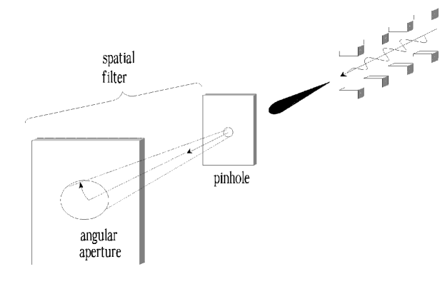
Figure 10: Undulator radiation with a pinhole spatial filter

The radiation is transversely coherent when

$$(\sigma_{\mathrm{e}})_{x,y}(\sigma^{\prime}_{\mathrm{e}})_{xy}\ll\lambda/(4\pi)\ ,\quad\beta\simeq L_{\mathrm{w}}\ .$$

Under these conditions, one has $(\sigma_{x,y})^{2}\ll(\sigma_{\mathrm{d}})^{2}$ and $(\sigma^{\prime}_{x,y})^{2}\ll(\sigma^{\prime}_{\mathrm{d}})^{2}$ and the spectral-angular dependence of the radiation emitted by an electron beam can be approximated by the spectral-angular dependence of the radiation emitted by a single electron. This limit corresponds to the maximum spectral brightness

$$B=\frac{4(\mathop{\mathrm{d}}N_{\mathrm{cen}}/\mathop{\mathrm{d}}t)(N_{\mathrm{w}}/1000)}{\lambda^{2}}\frac{{\mathrm{photons/s}}}{{\mathrm{mm}}^{2}{\mathrm{mrad}}^{2}{\mathrm{(0.1\%BW)}}}\ .$$

When the electron beam emittance is large,

$$(\sigma_{\mathrm{e}})_{x,y}(\sigma^{\prime}_{\mathrm{e}})_{xy}\gg\lambda/(4\pi)\ ,$$

the radiation is partially coherent. One can show that the influence of the electron beam divergence on the properties of the undulator radiation can be neglected when the beta-function is large enough. In the region of parameters when

$$(\sigma_{x,y}^{\prime})^{2}<(\sigma_{\mathrm{d}}^{\prime})^{2}$$

a downstream diaphragm of aperture $d=2\sigma_{\mathrm{d}}$ is used for selection of the transversely coherent fraction of undulator radiation. Finally, in this limit, the flux of transversely coherent photons into the bandwidth $\Delta\omega/\omega=0.1\%$ can be estimated simply as

$$\frac{\mathop{\mathrm{d}}N_{\mathrm{ph}}}{\mathop{\mathrm{d}}t}\simeq\frac{\lambda^{2}B}{4}\ .$$

These remarks may be useful in estimating the conditions under which a spatially coherent plane wavefront may be obtained from a noncoherent source.

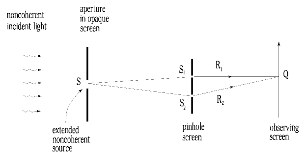
Figure 11: Young’s interferometer, for discussion of spatial coherence

5.4 Discussion of spatial coherence

The spatial coherence in a light beam generally has to do with the coherence between two points in the field illuminated by light source. The meaning of spatial coherence can best be understood with the help of Young’s two-pinhole experiment (see Fig. 11). In its elementary sense, the degree of coherence between the two points simply describes the contrast of the interference fringes that are obtained when the two points are taken as secondary sources. Let a source $S$ illuminate the two pinholes $S_{1}$ and $S_{2}$, as shown in Fig. 11. The source is perfectly noncoherent. That is to say, no interference fringes can be obtained by placing two pinholes in the plane of the source. It was shown, however, that if the two slits are placed far enough away from the noncoherent source, interference fringes of good contrast can be obtained (see Fig. 12). It is sometimes said that the spatial coherence in light beams increases with distance ”by mere propagation”. It would be nice to find an explanation which is elementary in the sense that we can see what is happening physically.

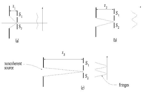
Figure 12: Interference-fringe amplitude, in Young’s interferometer, for three values of noncoherent source-pinhole screen distance

Suppose that a quasimonochromatic wave is incident on an aperture in an opaque screen, as illustrated in Fig. 13. In general, this wave may be partially coherent. The detailed structure of an optical wave undergoes changes at the wave propagates through space. In a similar fashion, the detailed structure of the spatial coherence undergoes changes, and in this sense the transverse coherence function is said to propagate. Knowing the spatial coherence on the aperture, we wish to find the spatial coherence on the observing screen at distance $z$ beyond the aperture. Synchrotron radiation is a stochastic object and for any synchrotron light beam there exist some characteristic linear dimension, $\Delta r_{\mathrm{c}}$, which determines the scale of spatially random fluctuations. Fig. 13 illustrates the type of spiky speckle pattern on an aperture in an opaque screen. When $\Delta r_{\mathrm{c}}\ll d$, the radiation beyond the aperture is partially coherent. This case is shown in Fig. 13. Here $\Delta r_{\mathrm{c}}$ may be estimated as the typical linear dimension of speckles.

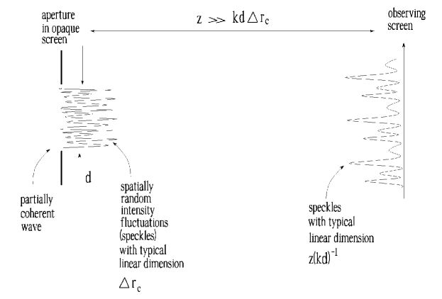
Figure 13: Geometry for propagation of spatial coherence

First we wish to calculate the (instantaneous) intensity distribution observed across a parallel plane at distance $z$ beyond the aperture. The observed intensity distribution can be found from a two-dimensional Fourier transform of the field. The radiation field across the aperture may be presented as a superposition of plane waves, all with the same wavenumber $k=\omega_{0}/c$. The value of $k_{\perp}/k$ gives the sine of the angle between the $z$ axis and the direction of propagation of the plane wave. In the paraxial approximation $k_{\perp}/k=\sin\theta\simeq\theta$. If the radiation beyond the aperture is partially coherent, a spiky angular spectrum is expected. The nature of the spikes in the angular spectrum is easily described in Fourier-transform notations. We can expect that the typical width of the angular spectrum envelope should be of the order of $(k\Delta r_{\mathrm{c}})^{-1}$. Also an angular spectrum of the source having transverse size $d$ should contain spikes with a typical width of about $(kd)^{-1}$, a consequence of the reciprocal width relations of Fourier transform pairs (see Fig. 14). It is the source linear dimension $d$ that determines the coherent area of the observed wave $z/(kd)$, but in addition the coherence linear dimension $\Delta r_{\mathrm{c}}$ of the source influences the distribution of average intensity over the observing screen with typical width $z/(k\Delta r_{\mathrm{c}})$. Thus, if the screen is placed far enough away from the noncoherent source, $z\gg d\Delta r_{\mathrm{c}}/\lambda$, a coherence area of large linear dimension can be obtained.

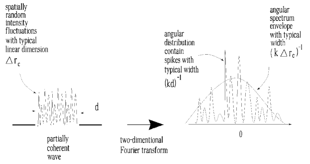
Figure 14: Reciprocal width relations of Fourier transform pairs

5.5 Grating monochromator considered as a spatial filter

In order to use the radiation from the source it first has to be filtered and monochromatized. Finally, to be complete, we should remark that in the experimental arrangement shown in Fig. 4 there is still one other effect which gives spatial filtering. A monochromator is just a spatial filter working in dispersive direction only. We would like to show next how it is that a monochromator can act like a spatial filter. Figure 15 shows the grating geometry under consideration. The finite size of the entrance and exit slits in the dispersive direction sets a limit to the achievable resolution. The slit-width-limited resolution can be obtained directly from the grating equation. In particular, the entrance slit-width-limited resolution is given by [9]:

$$\Delta\lambda=zd\cos(\alpha)/(nm)\ ,$$

where $\alpha$ is the angle of incidence, $N_{\mathrm{g}}$ is the number of lines on the grating, $D$ is the width of grating, $n=N_{\mathrm{g}}/D$ is the line density, $m$ is the order of the diffraction pattern, $d$ is the width of entrance slit, $z$ is the entrance slit-grating distance. We see that the resolution is equal to

$$\frac{\lambda}{\Delta\lambda}=\frac{zmN_{\mathrm{g}}\lambda}{Dd\cos(\alpha)}\ .$$

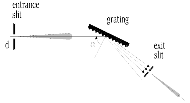
Figure 15: Illustration of grating monochromator. The finite size of the entrance slit in the dispersive direction sets a limit to the achievable resolution

The coefficient $(mN_{\mathrm{g}})^{-1}$ is just the minimal uncertainty in the wavelength that can be measured with the given grating. The coefficient of proportionality between $\lambda/\Delta\lambda$ and $mN_{\mathrm{g}}$ is $z\lambda/[Dd\cos(\alpha)]$. What does all this mean? This is an example in which transverse coherence plays an important role. The ability to spectrally filter radiation by a monochromator requires well-defined phase and amplitude variations of the fields across the grating. So in order that we shall have a sharp line in our spectrum corresponding to a definite wavelength with an uncertainty given by $(mN_{\mathrm{g}})^{-1}$, we have to have a wave transverse coherence area of at least the size $D\cos(\alpha)$. If the transverse coherence area is too small we are not using the entire grating. Suppose we have an entrance slit with aperture $d$ and send a beam of radiation at the grating with an aperture $D\cos(\alpha)$. The radiation reaching the grating is transversely coherent when the following condition for the space-angle product is fulfilled:

$$d\cdot\theta=Dd\cos(\alpha)/(2z)\simeq\lambda/(2\pi)\ .$$

We expect that only for pure transverse coherence, the grating will work right and the resolution $\lambda/\Delta\lambda$ and $mN_{\mathrm{g}}$ will be nearly equal. Importantly, in our scheme that incorporates an external pinhole spatial filter (see Fig. 4), the monochromator does not require an entrance slit.

5.6 Wave degeneracy parameter of undulator radiation

Physically the wave degeneracy parameter describes the average number of photons which can interfere, or, according to quantum theory, the number of photons in one quantum state (one ”mode”). We shall deal with two different approaches to the calculation of the wave degeneracy parameter. First we consider what can reasonably called ”fluctuation experiments in the frequency domain” (see subsection 3.6). For the frequency domain we use the notion of the wave degeneracy parameter $\delta_{\mathrm{W}}$ which is equal to the average number of transversely coherent photons radiated by the electron bunch inside the spectral interval of coherence $\Delta\omega_{\mathrm{c}}$. Taking into account that the ”emittance” of the diffraction limited photon beam is equal to

$$\min(\epsilon_{x,y})=\min(2\pi\sigma_{x,y}\sigma^{\prime}_{x,y})=\frac{\lambda}{2}\ ,$$

we calculate the average number of spatially coherent photons radiated within one pulse into the spectral interval of $\Delta\lambda/\lambda$:

$$(\Delta N_{\mathrm{ph}})_{\mathrm{coh}}=\frac{\lambda^{2}}{4}\frac{\Delta\lambda}{\lambda}\int^{\infty}_{-\infty}B(t)\mathop{\mathrm{d}}t\ ,$$

where $B(t)$ is the instantaneous spectral brightness of the synchrotron radiation. The value of $\Delta\lambda/\lambda$ is connected with the interval of the spectral coherence by the relation: $\Delta\lambda/\lambda=\Delta\omega_{\mathrm{c}}/\omega_{0}$. Using (16), (18) and Parseval’s theorem we obtain:

$$\frac{\Delta\omega_{\mathrm{c}}}{\omega_{0}}=\frac{1}{\omega_{0}}\int\limits^{\infty}_{-\infty}\mid g_{1}(\Delta\omega)\mid^{2}\mathop{\mathrm{d}}(\Delta\omega)=\frac{1}{\omega_{0}}\int\limits^{\infty}_{-\infty}\mid\bar{F}(\Delta\omega)\mid^{2}\mathop{\mathrm{d}}(\Delta\omega)=\frac{\lambda}{c}\int\limits^{\infty}_{-\infty}F^{2}(t)\mathop{\mathrm{d}}t\ .$$

Using the fact that the instantaneous spectral brightness $B(t)$ and the instantaneous value of the beam current $\langle I(t)\rangle$ are related by $B(t)\propto\langle I(t)\rangle$, we can equivalently write $B(t)={\mathrm{const}}.\times F(t)$. It is convenient to refer to the peak value of spectral brightness

$$\max(B)={\mathrm{const}}.\times\max(F)=B_{\mathrm{peak}}\ .$$

By convention, we represent the time integral of the instantaneous spectral brightness in the form

$$\int\limits^{\infty}_{-\infty}B(t)\mathop{\mathrm{d}}t={\mathrm{const}}.\times\int\limits^{\infty}_{-\infty}F(t)\mathop{\mathrm{d}}t=\frac{B_{\mathrm{peak}}}{\max(F)}\ .$$

Note that the dependence of the factor

$$A=\frac{1}{\max(F)}\int\limits^{\infty}_{-\infty}F^{2}(t)\mathop{\mathrm{d}}t$$

on the exact shape of the bunch is rather weak. The results are $A=1$ for the rectangular pulse-shape and $A=1/\sqrt{2}$ for the Gaussian pulse-shape. Thus $A\simeq 1$ is a reasonable approximation. Finally, the degeneracy parameter can be estimated simply as:

$$\delta_{\mathrm{W}}\simeq\frac{\lambda^{3}B_{\mathrm{peak}}}{4c}\ .$$ (52)

What about the other kinds of fluctuation experiments, for example, integrated intensity fluctuations? For the time domain we use the notion of the wave degeneracy parameter $\delta_{\mathrm{W}}$ which is equal to the average number of transversely coherent photons radiated by the electron bunch during the coherence time $\tau_{\mathrm{c}}$:

$$(\Delta N_{\mathrm{ph}})_{\mathrm{coh}}=\frac{\lambda^{2}}{4}\frac{\Delta\lambda}{\lambda}\left(\tau_{\mathrm{c}}B_{\mathrm{peak}}\right)\ .$$

Finally, the product $\tau_{\mathrm{c}}\Delta\lambda/\lambda$ is given by the expression

$$\tau_{\mathrm{c}}\Delta\lambda/\lambda=A^{\prime}\lambda/c\ .$$

The dependence of the factor $A^{\prime}$ on the exact shape of the spectral distribution is rather weak. Let us consider the specific case of a Gaussian line profile. The explicit expression for the coherence time is $\tau_{\mathrm{c}}=\sqrt{\pi}/\sigma_{\mathrm{m}}$. The FWHM bandwidth would be $\Delta\lambda/\lambda=2.36(\sigma_{\mathrm{m}}/\omega)$ giving, for $A^{\prime}=0.7$. Thus $A^{\prime}\simeq 1$ is a reasonable approximation and the wave degeneracy parameter $\delta_{\mathrm{W}}$ is given by the expression (52). The frequency domain calculations and time domain calculations give similar results.

Let us present a specific numerical example for the case of a third-generation synchrotron light source. The peak spectral brightness at a wavelength of 10 nm is equal to

$$B_{\mathrm{peak}}\simeq 10^{21}\frac{{\mathrm{photons/s}}}{{\mathrm{mm}}^{2}{\mathrm{mrad}}^{2}{\mathrm{(0.1\%BW)}}}\ .$$

Substituting this number into (52) we obtain that the wave degeneracy parameter is about $\delta_{\mathrm{W}}\simeq 10^{3}$. Hence in the soft X-ray region of the spectrum we expect classically induced fluctuations of photocounts to have a far stronger effect than pure quantum shot noise fluctuations. On the other hand, in the hard X-ray region of the spectrum ($\lambda\simeq 0.1$ nm), a source brightness in excess of

$$B_{\mathrm{peak}}\simeq 10^{24}\frac{{\mathrm{photons/s}}}{{\mathrm{mm}}^{2}{\mathrm{mrad}}^{2}{\mathrm{(0.1\%BW)}}}$$

is required to produce a wave degeneracy parameter greater than unity. Since third-generation sources have a peak brightness of only this value, we can conclude that in this region of the spectrum, the vast majority of third-generation synchrotron light sources encountered produce radiation with wave degeneracy parameters comparable with unity, and hence noise produced by the quantized nature of the radiation is comparable with the noise produced by classical fluctuations of the intensity.

A few additional comments are needed in closing this section. We have concentrated our attention on the wave degeneracy parameter, which is a property of the synchrotron radiation falling on the photodetector. That photodetector invariably has a quantum efficiency that is less than unity. In addition, the efficiency of the monochromator is less than unity, too. Hence the count degeneracy parameter will be even smaller than the wave degeneracy parameter. When the integration time is large, $\tau_{0}\gg\tau_{\mathrm{c}}$, the parameter $\delta_{\mathrm{c}}$ is given by:

$$\delta_{\mathrm{c}}=\eta R_{\mathrm{m}}\delta_{\mathrm{W}}\ .$$

where $R_{\mathrm{m}}$ is the monochromator throughput. In the opposite case, at $\tau_{0}\ll\tau_{\mathrm{c}}$, the parameter $\delta_{\mathrm{c}}$ is about

$$\delta_{\mathrm{c}}\simeq\eta R_{\mathrm{m}}(\Delta\omega_{\mathrm{m}}\tau_{0})\delta_{\mathrm{W}}\ .$$

In addition, it is possible that the sample or collecting optics may intercept only a fraction of one spatial mode from the source. In such a case the count degeneracy parameter may again be smaller than the wave degeneracy parameter, as a result of the incomplete capture of a spatial mode. Although the minimum value of $M$ is unity, the reduction of the energy striking the detector surface must be taken into account. In such a case, the count degeneracy parameter must be reduced from the normal value by a factor of the ratio of the effective measurement area to the coherence area of the incident light.

6 The signal-to-noise ratio associated with the output of the measurement system assumed for the pump-probe experiments

The principle of operation of the proposed pump-probe scheme is based essentially on the classical intensity fluctuations of synchrotron radiation. It is shown above that stochastic fluctuations of the classical intensity can influence the statistical properties of the photoevents that are observed. Note in particular that the variance $\sigma^{2}_{\mathrm{K}}$ of $K$ consists of two distinct terms, each of which has a physical interpretation:

$$\sigma^{2}_{\mathrm{K}}=\frac{\langle K^{2}\rangle-\langle K\rangle^{2}}{\langle K\rangle^{2}}=\frac{1}{\langle K\rangle}+\sigma^{2}_{\mathrm{W}}\$$ (53)

The first term is simply the variance of the counts that would be observed if the classical intensity were constant and the photocounts were purely Poisson. We refer to this contribution to the count fluctuations as ”quantum noise”. The second term, $\sigma^{2}_{\mathrm{W}}$, is clearly zero if there are no fluctuations of the classical intensity. For instance, in the case of laser light, this component would be identically zero, and the count variance would be simply that arising from Poisson-distributed counts. When synchrotron light is incident on the sample surface, the classical fluctuations are nonzero, and the variance of the photocounts is larger than that expected for a Poisson distribution by an amount that is proportional to the variance of the integrated intensity. This extra component of variance of the counts is often referred to as ”excess noise,” meaning that it is above and beyond that expected for pure Poisson fluctuations [4].

Our initial goal was to find expressions for the classical variance $\sigma^{2}_{\mathrm{W}}$ of the integrated intensity. Also of major interest is the signal-to-noise ratio, associated with the variance, which provides us with an indication of the magnitude of the fluctuations of classical variance relative to the expectation value. The general approach to calculating the output signal-to-noise ratio of the proposed device will be as follows. Following subtraction of the $\langle K\rangle$ associated with the quantum noise (see (53)), the signal-to-noise ratio takes the form

$$\frac{S}{N}=\frac{\sqrt{N_{\mathrm{shot}}}\sigma^{2}_{\mathrm{W}}\langle K\rangle^{2}}{\sqrt{\langle(K-\langle K\rangle)^{4}\rangle-\langle(K-\langle K\rangle)^{2}\rangle^{2}}}$$ (54)

where $\sigma^{2}_{\mathrm{W}}$ is calculated using (45), $N_{\mathrm{shot}}$ is the number of independent measurements averaged in the accumulator (total number of shots). The only requirement for the accuracy of this procedure is that the count fluctuations be uncorrelated from shot to shot, a property that does hold in our case.

A fully general study of the signal-to-noise ratio would be nontrivial. The difficulty arises in simultaneously including the effects on that noise of both the classically induced fluctuations and Poisson fluctuations of the counts. The full analysis, including both of these effects, is a difficult analytical problem. The calculation can be performed without great difficulty in two limiting cases, namely, the cases of degeneracy parameter very large and very small compared with 1. When $\delta_{\mathrm{c}}\gg 1$, there are many photoevents present in each coherence interval of the wave. The result is a ”bunching” of the photoevents by the classical intensity fluctuations, and an increase of the variance of the counts to the point where the classically induced fluctuations are far stronger than the quantum noise variations. When the degeneracy parameter is much larger than 1, the expression (54) can be replaced by

$$\frac{S}{N}=\frac{\sqrt{N_{\mathrm{shot}}}\langle(K-\langle K\rangle)^{2}\rangle}{\sqrt{\langle(K-\langle K\rangle)^{4}\rangle-\langle(K-\langle K\rangle)^{2}\rangle^{2}}}\quad{\mathrm{for}}\quad\delta_{\mathrm{c}}\gg 1\ .$$ (55)

Our consideration is restricted to the two simplest cases from the analytical point of view, namely, the cases of integration time $\tau_{0}$ very short and very long compared with the coherence time. For short integration time, the value of the incident intensity $I(t)$ is approximately constant over the entire counting interval. As a consequence, the integrated intensity $W$ is distributed in accordance with the negative exponential distribution (30). It follows that the $\langle K^{n}\rangle=\langle(\alpha W)^{n}\rangle$ can be expressed in terms of the mean as

$$\langle K^{n}\rangle/\langle K\rangle^{n}=n!\ .$$

Using the above expression, we find that the signal-to-noise ratio is given by the expression:

$$S/N\simeq\sqrt{N_{\mathrm{shot}}/8}\qquad{\mathrm{for}}\qquad\delta_{\mathrm{c}}\gg 1,\quad\tau_{\mathrm{c}}\gg\tau_{0}\ .$$ (56)

This calculation shows that the fluctuations of the $\langle(K-\langle K\rangle)^{2}\rangle$ is about $\sqrt{8}\simeq 3$ times larger than the fluctuations of the mean value $\langle K\rangle$.

At the opposite extreme, with an integration time much longer than the coherence time, the integrated intensity, $W$, is distributed in accordance with the Gaussian distribution. It follows that

$$S/N\simeq\sqrt{N_{\mathrm{shot}}/2}\qquad{\mathrm{for}}\qquad\delta_{\mathrm{c}}\gg 1,\quad\tau_{0}\gg\tau_{\mathrm{c}}\ .$$ (57)

We know that for the case when $\delta_{\mathrm{c}}\ll 1$ the fluctuations of photocounts are strongly dominated by pure quantum noise. Thus the probability of obtaining $K$ counts is, to a good approximation, given by the Poisson distribution. We cannot neglect the classically induced fluctuations of the counts when we calculate the signal component of the output, but we can neglect them when we calculate the noise, simply because their contribution to the noise is so small. For the final approximation we note that if the integration time $\tau_{0}$ is very short compared with the coherence time, the expression for the photocounts degeneracy parameter is equal to the average number of detected photoelectrons per pulse $\delta_{\mathrm{c}}\simeq\langle K\rangle$. Hence, when $\delta_{\mathrm{c}}\ll 1$ and $\tau_{0}\ll\tau_{\mathrm{c}}$ the following approximation is valid : $\langle K\rangle\ll 1$. As a reminder, recall that the factorial moments of the Poisson distribution are given by

$$\langle K(K-1)\cdots(K-n+1)\rangle=\langle K\rangle^{n}\ .$$

It follows that

$$\langle(K-\langle K\rangle)^{4}\rangle-\langle(K-\langle K\rangle)^{2}\rangle^{2}\simeq\langle K\rangle\qquad{\mathrm{for}}\quad\langle K\rangle\ll 1\ .$$

Substituting this result into (54) we find

$$S/N\simeq\delta^{3/2}_{\mathrm{c}}\sqrt{N_{\mathrm{shot}}}\qquad{\mathrm{for}}\qquad\delta_{\mathrm{c}}\ll 1\ ,\quad\tau_{0}\ll\tau_{\mathrm{c}}\ .$$

Note that this expression is independent of the integration time $\tau_{0}$. Therefore, the signal-to-noise ratio is not improved by using a longer ”characteristic time” of sample dynamics.

7 Pump-probe technique based on a correlation principle

A more complex instrument can be used to characterize the shape of the signal function. The technique we are to describe here is to use two spatially separated samples and record correlation of the count fluctuations for each value of the delay $\tau$ between two pump laser pulses. The new configuration is sketched in Fig. 16. In this case the transversely coherent probe X-ray beam is splitting and incidents on two spatially separated samples. The detected photoevents are than correlated, and the sample dynamics is determined from that correlation. Each detector is connected with a separate electronic counter. The version of apparatus for measurement of average count product depicted in Fig. 17. During one radiation pulse, each of two detectors registers $K_{1}$ and $K_{2}$ number of photocounts, respectively. After each shot, an electronic scheme multiplies these numbers and passes this product to an averaging accumulator, where it is added to the previously stored sum of count products. Finally, the total sum is divided by the number of shots. This result, averaged (shot to shot) count product $\langle K_{1}K_{2}\rangle$, contains information about the shape of the signal function. Another advantage of the correlator measurement is the possibility to remove the monochromator between spatial filter and sample and thus to increase the count degeneracy parameter.

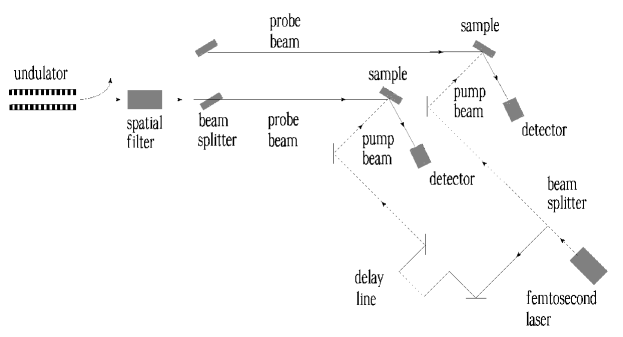
Figure 16: Scheme for pump-probe experiments employing correlator of count fluctuations

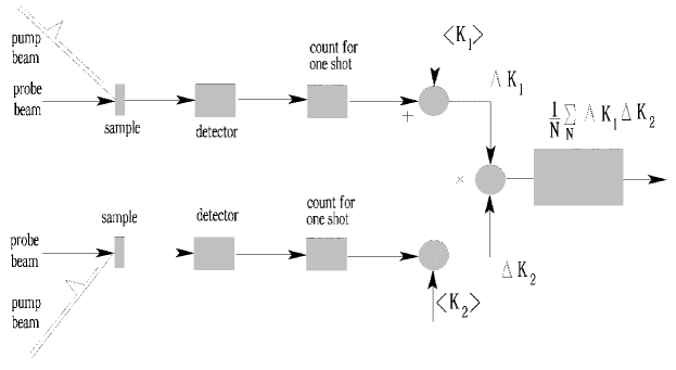
Figure 17: Correlation apparatus for analysis of sample dynamics

Now our goal is to find the relationship between the expected value of the average count product and the sample dynamics. In addition, we wish to find the variance of this quantity, so that the signal-to-noise ratio associated with the measurement can be determined and compared with the similar quantities found in the previous section.

7.1 The expected value of the count-fluctuation product and its relationship to the sample dynamics

By the ”count fluctuations” we mean explicitly the difference between the actual numbers of counts obtained in one shot at detector 1 and 2 and the expected values of these two number counts. Thus

$$\Delta K_{1}=K_{1}-\langle K_{1}\rangle\ ,\qquad\Delta K_{2}=K_{2}-\langle K_{2}\rangle\ .$$

The averaging accumulator at the output of the system depicted in Fig. 17 in effect produces an estimate of the expected value of the product of the two count fluctuations. Thus we are interested in statistical properties of the quantity $\langle\Delta K_{1}\Delta K_{2}\rangle$, and particular its mean and variance.

Let us calculate the expected average value of $\langle K_{1}K_{2}\rangle$:

$$\langle K_{1}K_{2}\rangle=\sum_{K_{1}=0}^{\infty}\sum_{K_{2}=0}^{\infty}K_{1}K_{2}P(K_{1},K_{2})\ ,$$

where $P(K_{1},K_{2})$ is the joint probability distribution of $K_{1}$ and $K_{2}$. It follows from the basic properties of the conditional probabilities that

$$P(K_{1},K_{2})=\int\limits^{\infty}_{0}\mathop{\mathrm{d}}W_{1}\int\limits^{\infty}_{0}\mathop{\mathrm{d}}W_{2}P(K_{1},K_{2}\mid W_{1},W_{2})P(W_{1},W_{2})\ ,$$

where $P(W_{1},W_{2})$ represents the joint probability distribution of integrated intensities $W_{1}$ and $W_{2}$. The values $W_{1,2}$ can be interpreted as the portion of X-ray pulse energy converted to a detectable form – photoelectrons for example (see section 2.7). Since $K_{1}$ and $K_{2}$ are independent when conditioned by the integrated intensities $W_{1}$ and $W_{2}$, respectively, we can write [4]:

$$P(K_{1},K_{2}\mid W_{1},W_{2})=P(K_{1}\mid W_{1})P(K_{2}\mid W_{2})\ ,$$

Using Mandel’s formula (46) we can write:

$$P(K\mid W)=\frac{(\alpha W)^{K}}{K!}\exp(-\alpha W)\ .$$

Using these facts, the following expression for the average of the count product can now be written

$$\langle K_{1}K_{2}\rangle=\sum^{\infty}_{K_{1}=0}\sum^{\infty}_{K_{2}=0}K_{1}K_{2}\int\limits^{\infty}_{0}\int\limits^{\infty}_{0}\frac{(\alpha W_{1})^{K_{1}}}{K_{1}!}\exp(-\alpha W_{1})\frac{(\alpha W_{2})^{K_{2}}}{K_{2}!}\exp(-\alpha W_{2})$$

$$\times P(W_{1},W_{2})\mathop{\mathrm{d}}W_{1}\mathop{\mathrm{d}}W_{2}\ .$$ (58)

At this point we interchange the orders of summation and integration in (58). Using the relationship

$$\sum^{\infty}_{K=0}K\frac{(\alpha W)^{K}}{K!}\exp(-\alpha W)=\alpha W\ ,$$

we can express the average of the count product in terms of the average of the classical integrated intensities at the two detectors [4],

$$\langle K_{1}K_{2}\rangle=\alpha^{2}\langle W_{1}W_{2}\rangle\ .$$

This result shows that much can be learnt about the classically induced fluctuations by studing the photocount correlation. So, the next problem is the description of the correlation of the classical integrated intensities

$$W_{1,2}=\int\limits^{\infty}_{-\infty}f_{1,2}(t)I_{1,2}(t)\mathop{\mathrm{d}}t\ ,$$

where $f(t)$ is the sample gating function (signal function). Suppose that the pump pulse interacts with the first and second sample at $t=0$ and $t=-\tau$, respectively. In this case the gating functions are: $f_{1}(t)=f(t),\quad f_{2}(t)=f(t+\tau)$. When the average intensities incident on the two samples are constant and equal,

$$\langle I_{1}(t)\rangle=\langle I_{2}(t)\rangle=\langle I\rangle={\mathrm{const.}}\ ,$$

the expression for the correlation of count fluctuations reduces to the useful form

$$\frac{\langle\Delta K_{1}\Delta K_{2}\rangle}{\langle K_{1}\rangle\langle K_{2}\rangle}=\frac{\langle\Delta W_{1}\Delta W_{2}\rangle}{\langle W_{1}\rangle\langle W_{2}\rangle}$$

$$=\frac{1}{\tau_{\mathrm{ch}}^{2}}\int\limits^{\infty}_{-\infty}\mathop{\mathrm{d}}t\int\limits^{\infty}_{-\infty}\mathop{\mathrm{d}}t^{\prime}f(t)f(t^{\prime}+\tau)\left[\frac{\langle I(t)I(t^{\prime})\rangle}{\langle I\rangle^{2}}-1\right]$$

$$=\frac{1}{\tau_{\mathrm{ch}}^{2}}\int\limits^{\infty}_{-\infty}\mathop{\mathrm{d}}t\int\limits^{\infty}_{-\infty}\mathop{\mathrm{d}}t^{\prime}f(t)f(t^{\prime}+\tau)\mid g_{1}(t-t^{\prime})\mid^{2}\ ,$$ (59)

where $\tau_{\mathrm{ch}}$ denotes:

$$\tau_{\mathrm{ch}}=\int\limits^{\infty}_{-\infty}f(t)\mathop{\mathrm{d}}t\ .$$

Then we remember that the behavior of $\mid g_{1}(t-t^{\prime})\mid^{2}$ for $\tau_{\mathrm{ch}}\gg\tau_{\mathrm{c}}$ approaches the behavior of the delta function (here $\tau_{\mathrm{ch}}$ is the ”characteristic time” of the sample dynamics). As a result we obtain

$$\frac{\langle\Delta K_{1}\Delta K_{2}\rangle}{\langle K_{1}\rangle\langle K_{2}\rangle}=\frac{\tau_{\mathrm{c}}}{\tau_{\mathrm{ch}}^{2}}\int\limits^{\infty}_{-\infty}f(t)f(t+\tau)\mathop{\mathrm{d}}t\qquad{\mathrm{for}}\qquad\tau_{\mathrm{ch}}\gg\tau_{\mathrm{c}}\ .$$ (60)

One can also write (60) as

$$\frac{\langle\Delta K_{1}\Delta K_{2}\rangle}{\langle K_{1}\rangle\langle K_{2}\rangle}=\sigma^{2}_{\mathrm{W}}\frac{\int\limits^{\infty}_{-\infty}f(t)f(t+\tau)\mathop{\mathrm{d}}t}{\int\limits^{\infty}_{-\infty}f^{2}(t)\mathop{\mathrm{d}}t}\ ,$$

where $\sigma^{2}_{\mathrm{W}}$ is the variance of the integrated intensity distribution ( for example see expression (45)). In the limit of a large photocount degeneracy parameter, $\delta_{\mathrm{c}}\gg 1$, we have $\sigma^{2}_{\mathrm{W}}\simeq\sigma^{2}_{\mathrm{K}}$.

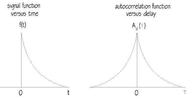
Figure 18: Some typical signal versus time and corresponding autocorrelation $A_{\mathrm{c}}(\tau)$

The expression

$$A_{\mathrm{c}}(\tau)=\int\limits^{\infty}_{-\infty}f(t)f(t+\tau)\mathop{\mathrm{d}}t$$

is called an autocorrelation. One immediately recognizes the physical meaning of the autocorrelation functions. The Fourier transform of the autocorrelation is $\bar{A}_{\mathrm{c}}(\omega)$, related to the Fourier transform of the signal by: $\bar{A}_{\mathrm{c}}(\omega)=\mid\bar{f}(\omega)\mid^{2}$. An autocorrelation is always a symmetric function. The Fourier transform of the autocorrelation is a real function, consistent with a symmetric function in the time domain. The question then naturally arises as to exactly what information about $f(t)$ can be derived from the measurement of cross-correlation (see Fig. 18). One can see that the proposed correlation technique provides the possibility to measure the modulus of the Fourier transform of the signal function, while information about its phase is missing. To provide reconstruction of the signal function from the autocorrelation function a special iterative technique should be used. Clearly, without loss of generality, we can assume that the signal function describing the sample dynamics is zero for $t<0$ and nonzero for $t>0$. Additionally we know that at $t=0$ the signal function is maximum. These relationships help us with the task at hand, namely determining the phase of $\bar{f}(\omega)$ from the knowledge of its modulus in the majority of cases involving functions $f(t)$ of considerable complexity. Nonetheless, it is possible to find cases in which ambiguities exist.

7.2 The signal-to-noise ratio associated with the output of the correlation apparatus

The signal-to-noise ratio for the proposed device (see Fig. 17) can be written in the form:

$$\frac{S}{N}=\frac{\sqrt{N_{\mathrm{shot}}}\langle\Delta K_{1}\Delta K_{2}\rangle}{\sqrt{\langle(\Delta K_{1}\Delta K_{2})^{2}\rangle-\langle\Delta K_{1}\Delta K_{2}\rangle^{2}}}\ ,$$ (61)

where $N_{\mathrm{shot}}$ is the number of independent measurements averaged in the accumulator. Let us consider the case when the degeneracy parameter is much larger than unity, $\delta_{\mathrm{c}}\gg 1$. The fluctuations of the photocounts are defined mainly by the classical noise in this case and (61) can be reduced to

$$\frac{S}{N}=\frac{\sqrt{N_{\mathrm{shot}}}\langle\Delta W_{1}\Delta W_{2}\rangle}{\sqrt{\langle(\Delta W_{1}\Delta W_{2})^{2}\rangle-\langle\Delta W_{1}\Delta W_{2}\rangle^{2}}}\ ,$$ (62)

Remembering that the integrated intensity is distributed in accordance with the Gaussian distribution one can derive that

$$\frac{\langle W_{1,2}^{2}\rangle}{\langle W_{1}\rangle^{2}}=1+\sigma^{2}_{\mathrm{W}}\ ,$$

$$\frac{\langle\Delta W_{1}\Delta W_{2}\rangle}{\langle W_{1}\rangle\langle W_{2}\rangle}=\sigma^{2}_{\mathrm{W}}A_{\mathrm{n}}(\tau)\ ,$$

$$\frac{\langle W_{1}^{2}W_{2}\rangle}{\langle W_{1}\rangle^{2}\langle W_{2}\rangle}=1+\sigma^{2}_{\mathrm{W}}+2\sigma^{2}_{\mathrm{W}}A_{\mathrm{n}}(\tau)\ ,$$

$$\frac{\langle W_{1}^{2}W_{2}^{2}\rangle}{\langle W_{1}\rangle^{2}\langle W_{2}\rangle^{2}}=1+2\sigma^{2}_{\mathrm{W}}+4\sigma^{2}_{\mathrm{W}}A_{\mathrm{n}}(\tau)+2\sigma^{4}_{\mathrm{W}}A^{2}_{\mathrm{n}}(\tau)+\sigma^{4}_{\mathrm{W}}\ ,$$ (63)

where $A_{\mathrm{n}}(\tau)$ denote

$$A_{\mathrm{n}}(\tau)=\frac{\int\limits^{\infty}_{-\infty}f(t)f(t+\tau)\mathop{\mathrm{d}}t}{\int\limits^{\infty}_{-\infty}f^{2}(t)\mathop{\mathrm{d}}t}\ .$$

Combining the above expressions, we find that the signal-to-noise ratio is given by the expression:

$$\frac{S}{N}=\frac{\sqrt{N_{\mathrm{shot}}}A_{\mathrm{n}}(\tau)}{\sqrt{1+A^{2}_{\mathrm{n}}(\tau)}}\qquad{\mathrm{for}}\qquad\delta_{\mathrm{c}}\gg 1\ .$$ (64)

Let us analyse the signal-to-noise ratio taking into account the quantum effects. When calculating the signal component (numerator of (61)), we can take into account classically induced fluctuations of the counts only. This can be done due to the fact that the quantum fluctuations of the counts at the outputs of two detectors are statistically independent. General calculations of the noise fluctuations associated with the output of the correlation apparatus (denominator of (61)) should include both the classical and the quantum effects. Taking into account these considerations we can derive the following relations:

$$\frac{\langle K_{1}^{2}K_{2}^{2}\rangle}{\langle K_{1}\rangle^{2}\langle K_{2}\rangle^{2}}=\frac{\langle(\alpha^{2}W_{1}^{2}+\alpha W_{1})(\alpha^{2}W_{2}^{2}+\alpha W_{2})\rangle}{\langle\alpha W_{1}\rangle^{2}\langle\alpha W_{2}\rangle^{2}}\ ,$$

$$\frac{\langle K_{1}^{2}K_{2}\rangle}{\langle K_{1}\rangle^{2}\langle K_{2}\rangle}=\frac{\langle(\alpha^{2}W_{1}^{2}+\alpha W_{1})\alpha W_{2}\rangle}{\langle\alpha W_{1}\rangle^{2}\langle\alpha W_{2}\rangle}\ ,$$

$$\frac{\langle K_{1,2}^{2}\rangle}{\langle K_{1,2}\rangle^{2}}=\frac{\langle\alpha^{2}W_{1,2}^{2}+\alpha W_{1,2}\rangle}{\langle\alpha W_{1,2}\rangle^{2}}\ .$$ (65)

We illustrate the technique for calculations of the above expressions for the value of $\langle K_{1}^{2}K_{2}^{2}\rangle$:

$$\langle K_{1}^{2}K_{2}^{2}\rangle=\sum_{K_{1}=0}^{\infty}\sum_{K_{2}=0}^{\infty}K_{1}^{2}K_{2}^{2}P(K_{1},K_{2})=$$

$$\int\limits_{0}^{\infty}\mathop{\mathrm{d}}W_{1}\int\limits\mathop{\mathrm{d}}W_{2}P(W_{1},W_{2})\times$$

$$\left[\sum_{K_{1}=0}^{\infty}K_{1}^{2}\frac{(\alpha W_{1})^{K_{1}}}{K_{1}!}\exp(-\alpha W_{1})\right]\times\left[\sum_{K_{2}=0}^{\infty}K_{2}^{2}\frac{(\alpha W_{2})^{K_{2}}}{K_{2}!}\exp(-\alpha W_{2})\right]=$$

$$\int\limits_{0}^{\infty}\mathop{\mathrm{d}}W_{1}\int\limits\mathop{\mathrm{d}}W_{2}P(W_{1},W_{2})(\alpha^{2}W_{1}^{2}+\alpha W_{1})(\alpha^{2}W_{2}^{2}+\alpha W_{2})=$$

$$\langle(\alpha^{2}W_{1}^{2}+\alpha W_{1})(\alpha^{2}W_{2}^{2}+\alpha W_{2})\rangle\ .$$ (66)

We will consider only the special case when the degeneracy parameter is much less than 1. Using the approximation $\delta_{\mathrm{c}}\ll 1$ we obtain $(\delta_{\mathrm{c}})_{1,2}\simeq\langle K_{1,2}\rangle$. Under such condition one would have, from (65), the variance

$$\langle(\Delta K_{1}\Delta K_{2})^{2}\rangle-\langle\Delta K_{1}\Delta K_{2}\rangle^{2}\simeq\langle K_{1}K_{2}\rangle\ ,$$

and the signal-to-noise ratio would be

$$\frac{S}{N}=\sqrt{N_{\mathrm{shot}}}\delta_{\mathrm{c}}A_{\mathrm{n}}(\tau)\qquad{\mathrm{for}}\qquad\delta_{\mathrm{c}}\ll 1\ .$$ (67)

The analysis of the obtained asymptotic expressions (64) and (67) for the signal-to-noise ratio allows one to make the following conclusions:

(i) The signal-to-noise ratio depends on the degeneracy parameter only when $\delta_{\mathrm{c}}$ is much less that 1. In this case the number of independent measurements for a given signal-to-noise ratio is proportional to $(1/\delta_{\mathrm{c}})^{2}$.

(ii) The signal-to-noise ratio is proportional to $A_{\mathrm{n}}(\tau)$. To hold the signal-to-noise ratio constant, the number of independent measurements must be proportional to $A^{-2}_{\mathrm{n}}(\tau)$.

7.3 Other autocorrelation techniques

There are other techniques to provide the possibility to measure the integrated intensity autocorrelation. They differ from each other in the beam splitters, the delay line and the detection system. We will now describe two new approaches. An alternative technique to generate $A_{\mathrm{n}}(\tau)$ is to use one pump beam and two probe beams. In the setup shown in Fig. 19 the pump pulse perturbs the sample at time $t=0$. A long X-ray pulse passes a beam splitter, generating two pulses travelling different paths. After the two paths are recombined, the two pulses impinge on the sample at a time difference $\tau$ which can be varied. The photocounts are recorded by a detector and the variance $\sigma^{2}_{\mathrm{K}}$ is studied as a function of $\tau$.

Now we describe the basic principles of autocorrelation measurement with this arrangement. In the limit of a large photocount degeneracy parameter the expression for the variance of counts reduces to the form ($\langle I_{1}\rangle=\langle I_{2}\rangle$ = const.):

$$\frac{\langle(\Delta K)^{2}\rangle}{\langle K\rangle^{2}}=\frac{\langle(\Delta W)^{2}\rangle}{\langle W\rangle^{2}}$$

$$=\frac{1}{\tau_{\mathrm{ch}}^{2}}\int\limits^{\infty}_{-\infty}\mathop{\mathrm{d}}t\int\limits^{\infty}_{-\infty}\mathop{\mathrm{d}}t^{\prime}f(t)f(t^{\prime})\left\{\frac{\langle[I_{1}(t)+I_{2}(t+\tau)][I_{1}(t^{\prime})+I_{2}(t^{\prime}+\tau)]\rangle}{\langle(I_{1}+I_{2})\rangle^{2}}-1\right]$$

$$=\frac{1}{2\tau_{\mathrm{ch}}^{2}}\int\limits^{\infty}_{-\infty}\mathop{\mathrm{d}}t\int\limits^{\infty}_{-\infty}\mathop{\mathrm{d}}t^{\prime}f(t)f(t^{\prime})\left[\mid g_{1}(t-t^{\prime})\mid^{2}+\mid g_{1}(t-t^{\prime}+\tau)\mid^{2}\right]\ .$$ (68)

Remembering that the behavior of $\mid g_{1}(t-t^{\prime})\mid^{2}$ for $\tau_{\mathrm{ch}}\gg\tau_{\mathrm{c}}$ approaches the behavior of the delta function we obtain

$$\sigma^{2}_{\mathrm{W}}(\tau)=\frac{1}{2}\left[\frac{\tau_{\mathrm{c}}}{\tau_{\mathrm{ch}}^{2}}\int\limits^{\infty}_{-\infty}f^{2}(t)\mathop{\mathrm{d}}t\right]\left[1+A_{\mathrm{n}}(\tau)\right]\qquad{\mathrm{for}}\qquad\tau_{\mathrm{ch}}\gg\tau_{\mathrm{c}}\ .$$ (69)

One can also write (69)

$$\sigma^{2}_{\mathrm{W}}(\tau)=\frac{1}{2}\sigma^{2}_{\mathrm{W}}(0)\left[1+A_{\mathrm{n}}(\tau)\right]\ ,$$

where $\sigma^{2}_{\mathrm{W}}(0)$ is the variance of the integrated intensity distribution for the single probe beam:

$$\sigma^{2}_{\mathrm{W}}(0)=\frac{\tau_{\mathrm{c}}}{\tau_{\mathrm{ch}}^{2}}\int\limits^{\infty}_{-\infty}f^{2}(t)\mathop{\mathrm{d}}t\ .$$

At $\tau=0$, the peak value of the function $\sigma^{2}_{\mathrm{W}}(\tau)$ is $\sigma^{2}_{\mathrm{W}}(0)$. For large delays compared to the ”characteristic time” of the sample dynamics, the cross product term vanishes, leaving a background of $\sigma^{2}_{\mathrm{W}}(\infty)=\sigma^{2}_{\mathrm{W}}(0)/2$. The variance as a function of delay time has thus a peak to background of 2 to 1. The measurement leading to $\sigma^{2}_{\mathrm{W}}(\tau)$ we can refer to as the integrated intensities autocorrelation with background, as opposed to the background free autocorrelation described in the previous subsection (see Fig. 16).

The most important and critical area of R&D for time-resolved experiments utilizing the autocorrelator will be the development of X-ray beam splitters and delay lines. Considerable work will need to be undertaken to make them routinely used optical elements.

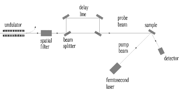
Figure 19: Scheme for autocorrelation pump-probe experiments employing two probe beams originating from the splitting of a single X-ray beam produced by an undulator (with one partial beam delayed relative to the other)

Figure 20: Scheme for autocorrelation pump-probe experiments employing two probe beams that are generated by the same electron bunch but from two undulators

The technique to use two probe X-ray beams that are generated by the same electron bunch but from two insertion devices (again with one beam delayed with respect to the other) may be a more promising approach. The concept is very interesting in view of the critical synchronization of probe beams (see Fig. 20). Using this technique precisely controlled temporal resolution down to several femtoseconds should be achievable. To delay the electron beam, a small magnetic chicane has to be applied. The trajectory of the electron beam in the chicane has the shape of an isosceles triangle with the base equal to $L$. The angle adjacent to the base, $\theta$, is considered to be small. The optimal parameters of the chicane can be calculated in the following way. The electron beam delay line needed for time resolved experiments has to satisfy two requirements. First, the electron beam extra path length, $L\theta^{2}/2$, must be long enough to reach a delay time of about 100 femtoseconds. A first question that arises is: why do we want to use 100 fs delay time? Here we direct the attention of the reader to the fact that we assume to use 5-10 fs visible pump pulses. On the other hand we assume that the pump pulse can be approximated by a delta function. One can never hope to achieve a visible laser pulse duration ten times shorter than the present. This limitation prevents the application of this technique to the timescale shorter than 100 fs.

Second, the effect of suppressing the beam density modulation due to the presence of the energy spread in the electron beam should be avoided in order to preserve the correlation of the radiation field within the delay time. The energy spread suppresses significantly the microbunching when $\omega_{0}L\theta^{2}\Delta\gamma/(c\gamma)$ is larger than or equal to unity. Parameters in our case are: $\Delta\gamma/\gamma\simeq 10^{-3}$, $L\theta^{2}\simeq 60\mu{\mathrm{m}}$. The delay time and energy spread in the electron beam dictates the choice of synchrotron radiation wavelengths. These results demonstrate that this scheme is adequate for the VUV spectral range, but cannot be used to produce X-ray probe beams. The situation is quite different for the first scheme of autocorrelator (see Fig. 19). Since in this case the probe beams are produced by X-ray splitter and delay line, the energy spread limitation does not exist at all.

8 Concluding remarks

A general objective in the development of synchrotron radiation sources is to produce radiation that is brighter than that from existing sources, or to produce radiation that comes in shorter pulses. Current machines produce bunch lengths in the 100-ps regime. Many experiments exploit this time dependence. Light-triggered time-resolved studies with 100 ps resolution are now frequently performed at synchrotron light sources. However, 100 picoseconds is longer than the time associated with many interesting physical phenomena. The storage ring technology itself approaches its limits of performance with respect to minimal pulse duration. No practical means have been found to allow bunches of less than a ten picoseconds duration to be stored. A proposed in this paper schemes for fast time-resolved experiments could offer the possibility to overcome this limitation. It was shown that the femtosecond timescale associated with intensity fluctuations in synchrotron light pulses make them well suited for time-resolved studies. The new concept eliminates the need for ultrashort X-ray pulses. This development in synchrotron based pump-probe experiments allows us to investigate phenomena in the time range down to 100 fs. It is the author’s hope that the general principles of pump-probe techniques based on statistical properties of synchrotron light, presented in this paper, may help in stimulating further inquiry and result in success in many exciting applications, some of which can now only be barely envisioned.

References

- [1] C. Rulliere (Ed.) ”Femtosecond Laser Pulses” (Springer, Berlin, 1998)
- [2] A. Rousse, C. Rischel and J.-C. Gauther, Rev. Mod. Phys., Vol. 73, No. 1, January 2001
- [3] R. Loudon , ”The Quantum Theory of Light” (Clarendon Press, Oxford, 1973)
- [4] J. Goodman, ”Statistical Optics” (Wiley, New York, 1985)
- [5] E. L. Saldin, E. A. Scheidmiller and M. V. Yurkov, ”The Physics of Free Electron Lasers” (Springer, Berlin, 1999)
- [6] P. W. Milonni, ”The Quantum Vacuum” (Academic Press, Inc., New York, 1994)
- [7] H. Wiedemann, Particle Accelerator Physics” (Springer, Berlin, 1995)
- [8] D. Attwood, ”Soft X-ray and Extreme Ultraviolet Radiation” (Cambridge University Press, 1999)
- [9] J. B. West and H. A. Padmore ”Optical Engineering” (Handbook on Synchrotron Radiation, Vol. 2, Elsevier Science Publishers B. V., 1987)