Scaling limit of virtual states of triatomic systems

Abstract

For a system with three identical atoms, the dependence of the $s-$wave virtual state energy on the weakly bound dimer and trimer binding energies is calculated in a form of a universal scaling function. The scaling function is obtained from a renormalizable three-body model with a pairwise Dirac-delta interaction. It was also discussed the threshold condition for the appearance of the trimer virtual state.

PACS 03.65.Ge, 11.80.Jy, 21.45.+v, 21.10.Dr

I Introduction

Weakly bound three-body zero-angular momentum states appear in a three boson system, with the number of states growing to infinity, condensing at zero energy as the pair interactions are just about to bind two particles in $s-$wave. These three-body states are known as Efimov states [1, 2]. Their wave functions, loosely bound, extend far beyond those of normal states and dominate the low-energy scattering phenomena in these systems. The Efimov states have been studied in a number of model calculations [3, 4, 5], in atomic and nuclear systems, without yet a clear experimental signature of their occurrence [2, 6, 7, 8, 9, 10].

Actually, the search of Efimov states in atomic systems is becoming more appealing, due to the experimental realization of Bose-Einstein condensation (BEC) [11], and due to the possibility of altering the effective scattering length of the low-energy atom-atom interaction in the trap, from large negative to large positive values crossing the dimer zero binding energy value, by using an external magnetic field [12]. This possibility of changing the two-body scattering length to large values, as recently shown in Ref. [13], can alter in an essential way the balance between the non-linear first few terms of the mean-field description presented in the equations that model Bose-Einstein condensed gases [14]. This can certainly open new perspectives for theoretical and experimental investigations related to the many-body behavior of condensate systems. Even in systems where the occurrence of an excited bound Efimov state has shown to be doubtful or even not possible, as for example, in the case of halo nuclei like ²⁰C or ¹⁸C (seen as a core with a halo of two neutrons) [8], one can verify the occurrence of three-body virtual states. The physics of these three-body systems is related to the unusually large size of the wave-function compared to the range of the potential. Thus, the detailed form of the short-ranged potential is not important for the three-body observables[15], which gives to the system universal properties, defined by few physical scales[8]. Strictly speaking, in the limit of a zero-range interaction the three-body system is parametrized by the physical two- and three-body scales, which are identified with the two-body scattering lengths and one three-body binding energy [9, 16]. The physical reason for the sensibility of the three-body binding energy to the interaction properties comes from the collapse of the system in the limit of a zero-range force, which is known as the Thomas effect [17].

In the present work, we analyze the possibility that an excited trimer state becomes a virtual state, when the physical scales of the system are changed. This is expected to occur, for example, near the limit when the two-body scattering length goes from large positive to large negative value: the corresponding two-body energy is close to zero and goes from a bound to a virtual state, with appearance of many bound and virtual three-body states. The three-body virtual state energy is a pole of the S-matrix in the second sheet of the complex energy plane. In a general case, as the strength of the two-body potential diminishes, the pole moves towards the first energy sheet to become a bound state [5]. More recently, this behavior of the Efimov state going to a virtual state with the increase of the strength of the interaction, has been confirmed in realistic calculation of the helium trimer [18]. Here, we study a new physical aspect of the emergence of the $s-$wave virtual state from an Efimov state: it appears when the ratio between the dimer and trimer binding energies grows. This approach goes beyond a previous analysis of excited three-body bound states with short-range interactions, that was performed in Ref. [9]. In Ref. [9], a scaling function was introduced to analyze the behavior of bound Efimov states when modifying the triatomic physical scales. Essentially, we are extending to the second sheet of the complex energy plane (to include virtual trimer states) a previous investigation on a universal scaling mechanism that was applied to two and three-body bound states[9, 10]. The extension of the scaling function to the second energy sheet is performed by following the Efimov states as they move from bound to virtual, accordingly to the variation of the ratio of the dimer to trimer bound state energies. On the other hand, as we present the discussion through a universal scaling mechanism with the results in dimensionless units, all the conclusions apply equally to any low-energy three-boson system. For the regularization and renormalization of the zero-range model, we compare two different approaches: by using a momentum cutoff parameter [9] and via kernel subtraction [16, 19, 20]. As the two-body energy goes to zero (or equivalently the regularization parameter goes to infinity), we conclude that the results of both methods do not differ.

The paper is organized as follows. In section II, we generalize the scaling function defined in Ref. [9] to include virtual trimer states. In this section, we also revise the connection between the Thomas and Efimov effects, while introducing our notation and the homogeneous integral equation for the Faddeev component of the vertex of the wave-function for zero-range potential. In section III we present our main numerical results. In the first subsection, we present the subtracted homogeneous Faddeev equation that we have used for determining the trimer bound and virtual states and we briefly explain how the renormalization method of Refs. [19, 20] implies in the subtracted three-body equation first formulated in Ref. [16]. In the next subsection, we present our new numerical results for the virtual state energies, including the bound-state previous results and we compare, as well, the results obtained by using the sharp-cutoff and the subtraction scheme. Comparison with other calculations are also discussed. Our conclusions are summarized in section IV.

II Thomas-Efimov Effect and the Generalized Scaling Function

In this section, we introduce the generalization of the scaling function defined in Ref. [9], to be used in the second energy sheet of the trimer energy. In order to become clear this extension, and to define our notation, we begin by revising the main findings of Refs. [9, 21].

The two-boson system in the limit of a zero-range interaction has only one physical scale, that one can choose the scattering length ($a$) or the energy of the bound or virtual state. The two-body $s-$wave scattering amplitude in units of $\hbar=m=1$ is parametrized as a function of the momentum $k$, by $f(k)=\left(k\cot\delta_{0}-{\rm i}k\right)^{-1},$ where the $s-$wave phase shift $\delta_{0}$ is given by $k\cot\delta_{0}=-a^{-1}+\frac{1}{2}r_{0}k^{2}+...,$ and $r_{0}$ is the effective range. For $a\ >\ 0$ the two-body system is bound, otherwise, for $a\ <\ 0$, it is virtual. A short range potential is characterized by $r_{0}|a|^{-1}<<1$ and, in this case, $f(k)=\left(-a^{-1}-{\rm i}k\right)^{-1}$ and $a^{-1}=\pm\sqrt{E_{2}}$ ($+$ for bound and $-$ for virtual state).

The three-boson system for $\ell=0$ in three dimensions collapses when $r_{0}\rightarrow 0$ with a fixed two-body scale, which is known as Thomas effect[17]. Thus, the three-body system has a characteristic physical scale independent of the two-body ones[16]. In one and two space dimensions the collapse is absent[15]. In the limit when the binding energy of the two-boson system goes to zero, the three-boson system has an infinite number of bound Efimov states [1] condensing at zero-energy. The Thomas and Efimov effects were shown to be physically equivalent [21], since in both cases the ratio between the interaction range and the two-body scattering length goes to zero.

The integral equation for the Faddeev components, $\phi$, of the three boson bound state vertex, for $\ell=0$, with the zero-range interaction, needs a momentum cut-off $(\Lambda$) of the order of $r_{0}^{-1}$, due to the Thomas collapse. According to Ref.[21], using units of $\Lambda=1$, we rescale the momentum variables and the two and three-body binding energies, respectively, such that $\vec{p}=\Lambda\vec{x}$, $\vec{q}=\Lambda\vec{y}$, $E_{2}=\Lambda^{2}\epsilon_{2}$, and $E_{3}=\Lambda^{2}\epsilon_{3}$. In this dimensionless variables, after redefining $\phi$ as $\chi(\vec{x})\equiv\Lambda^{3/2}\phi(\vec{p})$, we obtain the integral equation [21, 7, 8]:

$$\chi(\vec{y})=\frac{-\pi^{-2}}{\pm\sqrt{\epsilon_{2}}-\sqrt{\epsilon_{3}+\frac{3}{4}\vec{y}^{2}}}\int d^{3}x\;\frac{\theta(1-|\vec{x}|)}{\epsilon_{3}+\vec{y}^{2}+\vec{x}^{2}+\vec{y}.{\vec{x}}}\;\chi(\vec{x})\ .$$ (1)

The number of three-body bound states, given by the values of $\epsilon_{3}$ that satisfies Eq. (1), grows without limit when $\epsilon_{2}$ decreases to zero: $\epsilon_{3}=\epsilon_{3}^{(N)}$ $(N=0,1,2...)$, with $\epsilon_{3}^{(N)}/\epsilon_{3}^{(N+1)}\approx$ 500 [1]. They are the energies of the Efimov states, in units of $\Lambda=1$. But, the limit of $\epsilon_{2}$ going to zero, can be realized either by $E_{2}\rightarrow 0$ (with a fixed $\Lambda$) or by $\Lambda\sim r_{0}^{-1}\rightarrow\infty$ (with $E_{2}$ fixed). In this last case, the range of the interaction is set to zero and the system collapses: $E_{3}^{(0)}=\epsilon_{3}^{(0)}\Lambda^{2}\to\infty$. This is known as the Thomas collapse of the three-body ground state. Therefore, the Thomas and the Efimov states are given by the same limit $\epsilon_{2}\to 0$ of Eq. (1), and are related by a scale transformation[21].

Now, the concept of the scaling function is introduced according to Ref.[9]. For a nonvanishing $\epsilon_{2}$, the solutions of Eq. (1) defines the dimensionless three-body energies as functions of $\pm\sqrt{\epsilon_{2}}$: $\epsilon_{3}^{(N)}\equiv\epsilon_{3}^{(N)}\left(\pm\sqrt{\epsilon_{2}}\right)\$. Using the $N-$th energy to obtain $\Lambda$, then $\Lambda^{2}=E_{3}^{(N)}/\epsilon^{(N)}_{3}$, and

$$E_{3}^{(N+1)}=E_{3}^{(N)}\ .\ \frac{\epsilon_{3}^{(N+1)}\left(\xi\right)}{\epsilon_{3}^{(N)}}\ ,$$ (2)

where $\xi\equiv\pm\sqrt{\epsilon_{2}}=\pm{\left(E_{2}\;\epsilon^{(N)}_{3}/E^{(N)}_{3}\right)^{1/2}}$. In Eq.(2), the two and three body physical scales determines $E^{(N+1)}_{3}$, the next excited state above $E^{(N)}_{3}$. In Ref. [9], $E^{(N)}_{3}$ was identified with the three-body scale, as any state $N$ works equally well to set the trimer scale. However, we will be interested in the two most excited three-body states, that in practice we are going to identify with the ground and first excited state in triatomic systems. This identification is unambiguous because, with $N$ and $N+1$ two consecutive excited states, the limit

$$\frac{E_{3}^{(N+1)}}{E_{3}^{(N)}}\ =\ \lim_{N\rightarrow\infty}\frac{\epsilon_{3}^{(N+1)}\left(\xi\right)}{\epsilon_{3}^{(N)}}\ =\ {\cal F}\left(\pm\sqrt{\frac{E_{2}}{E^{(N)}_{3}}}\right)$$ (3)

exists and defines the scaling function ${\cal F}$[8, 9]. A qualitative argument to explain the scaling limit has been provided in Ref. [9] based on the notion of the long-range potential [1, 2, 22].

In the next, we provide the generalization of the scaling function (3), that is obtained by extending the formalism to the second sheet of the three-body complex energy plane. In the present approach, we only consider the two-body subsystem as bound. For this purpose, we define the general scaling function ${\cal K}$, given by

$$\ {\cal K}\left(\sqrt{\frac{E_{2}}{E^{(N)}_{3}}}\right)\ \equiv\pm\sqrt{\frac{E_{3}^{(N+1)}-E_{2}}{E_{3}^{(N)}}}\ =\pm\sqrt{\frac{\epsilon_{3}^{(N+1)}-\epsilon_{2}}{\epsilon_{3}^{(N)}}}\ .$$ (4)

This defined function ${\cal K}$ has its values on the imaginary axis of a three-body momentum space; a space that is defined with origin at the point in which the energies of the three-body system and the bound two-body subsystem are equal($E_{3}=E_{2}$). In this respect, relative to the bound subsystem, we can define bound and virtual states for the three-body system: ${\cal K}$ assumes a negative value for a three-body virtual state; and a positive value for a three-body bound-state. Schematically, we represent in Fig. 1 the energies of the two- and three- body system in the complex energy plane. The two-body subsystem is bound and the three-body system can be bound or virtual, with the energies given, respectively by $\epsilon_{3B}$ and $\epsilon_{3V}$. Through the elastic cut (corresponding to the atom-dimer elastic scattering) one defines two-sheets; in the first sheet, we have the three-body bound state energy at Re$(\epsilon)=-\epsilon_{3B}$; in the second sheet, the three-body virtual state energy at Re$(\epsilon)=-\epsilon_{3V}$, as illustrated in Fig. 1.

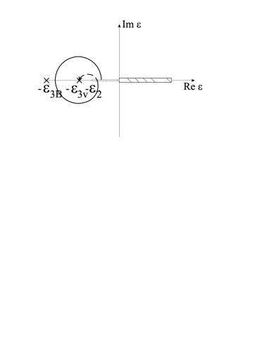
FIG. 1.: Schematical representation of the complex energy plane, in our dimensionless units. $\epsilon_{3B}$ and $\epsilon_{3V}$ are, respectively, pictorial representations of the positions of the three-body bound- and virtual-state energies in the first and second three-body energy sheet. The three-body cut is shown for Re$(\epsilon)>0$. The elastic cut (the narrow one) is shown with the origin at Re$(\epsilon)=-\epsilon_{2}$, where $\epsilon_{2}$ is the energy of the two-body bound state.

We would like to add one more comment to this section. The existence of a three-body scale implies in the low energy universality found in three-body systems, or correlations between three-body observables [23, 16]. In the scaling limit, one has

$${\cal{O}}\left(E,E_{3},E_{2}\right)=(E_{3})^{\eta}{\cal A}\left(\sqrt{E/E_{3}},\sqrt{E_{2}/E_{3}}\right)\ ,$$ (5)

where $\cal O$ is a general observable of the three-body system at energy $E$, with dimension of energy to the power $\eta$. The scattering amplitude of the elastic process a + bc $\rightarrow$ a + bc, $f_{3}=\sqrt{E_{3}}^{-1}\;F(\sqrt{E/E_{3}},\sqrt{E_{2}/E_{3}})$ for $E=E_{2}$, implies that the scattering length is given by a function $a_{3}=\sqrt{E_{3}}^{-1}\;F(\sqrt{E_{2}/E_{3}})$. In the three-nucleon system this originates the “Phillips plot”, the correlation between the doublet neutron-deuteron scattering length and the triton energy [24]. The scaling functions Eqs. (3) and (4) express the correlation between the excited or virtual state energies of the trimer and its ground state energy, which can be understood as particular cases of Eq. (5).

III Numerical Results for Virtual and Bound Trimers

In this section we present our main results for the trimer bound and virtual states. With the sake to be complete, we first briefly sketch a new derivation of the subtracted equations that were numerically solved.

A Renormalization and Subtracted Equations

The homogeneous form of the subtracted Faddeev equation [16] for the bound three-boson system with a zero-range interaction, is given by:

$$\chi(\vec{y})=\frac{-\pi^{-2}}{\pm\sqrt{\epsilon_{2}}-\sqrt{\epsilon_{3}+\frac{3}{4}\vec{y}^{2}}}\int d^{3}x\left(\frac{1}{\epsilon_{3}+\vec{y}^{2}+\vec{x}^{2}+\vec{y}.{\vec{x}}}-\frac{1}{1+\vec{y}^{2}+\vec{x}^{2}+\vec{y}.{\vec{x}}}\right){\chi(\vec{x})}\ ,$$ (6)

which is written in units such that the three-body subtraction energy is $\mu_{(3)}^{2}=1$. It has a similar form as Eq.(1) with a different regulator, that expresses the physical condition at the subtraction point.

We briefly explain below the main physical steps to derive the three-body renormalized equation [16] used in our numerical calculation of the scaling functions through Eq.(6) for the bound state and its analytic continuation to the second energy sheet for the virtual state. We begin from the general Lippman-Schwinger equation expressed in a subtracted form [19]:

$$T_{\cal R}(E)=T_{\cal R}(-\mu^{2})+T_{\cal R}(-\mu^{2})\ \left[G^{(+)}_{0}(E)-G_{0}(-\mu^{2})\right]T_{\cal R}(E),$$ (7)

where $T_{\cal R}(-\mu^{2})$, which is the T-matrix at a given energy scale $-\mu^{2}$ (negative energy, for convenience), $G_{0}^{(+)}(E)=[E-H_{0}+{\rm i}\delta]^{-1}$ and $H_{0}$ is the free Hamiltonian. Equation (7) defines the renormalized T-matrix in which $T_{\cal R}(-\mu^{2})$ is known and replace the original ill-defined potential $V$:

$$T_{\cal R}(-\mu^{2})=\left[1-VG_{0}(-\mu^{2})\right]^{-1}V\ .$$ (8)

The renormalized T-matrix does not depend on the arbitrary subtraction point $-\mu^{2}$ (once ${dV}/{d\mu^{2}}=0$), which implies in a Callan-Symanzik [19, 20] type equation for $T_{\cal R}(-\mu^{2})$:

$$\frac{d}{d\mu^{2}}T_{\cal R}(-\mu^{2})=T_{\cal R}(-\mu^{2})\left[G_{0}(-\mu^{2})\right]^{2}T_{\cal R}(-\mu^{2})\ .$$ (9)

This expresses the renormalization group invariance of the subtracted equation.

To solve Eq.(7) for the three-body T-matrix, $T^{(3)}_{\cal R}(E)$, a dynamical assumption has to be made at a particular subtraction point $-\mu^{2}_{(3)}$, where we assume that the three-body T-matrix is equal to the driving term, which is given by the sum of the pairwise two-body T-matrices. Thus, at the energy $-\mu^{2}_{(3)}$ it is assumed that the three-body multiple scattering series vanishes beyond the driving term. Observe that this is not true for a regular finite range potential, only in the limit of $\mu_{(3)}\rightarrow\infty$. However, in the scaling limit, in fact the actual value of $\mu_{(3)}$ tends to infinity such that $E_{2}/\mu^{2}_{(3)}$ goes to zero, as it be will be clear in our numerical calculations.

With our assumption, the T-matrix at the subtraction point $\mu_{(3)}$ is given by

$$T^{(3)}_{\cal R}(-\mu_{(3)}^{2})=\sum_{(ij)}T^{(2)}_{{\cal R}(ij)}\left(-\mu_{(3)}^{2}-\frac{q^{2}_{k}}{2m_{k(ij)}}\right),$$ (10)

where $(i,j,k)=(1,2,3),\;(2,3,1),\;(3,1,2)$. The summation is performed over all pairs and the renormalized two-body T-matrix elements for the pair $(ij)$ are given by $\langle{\vec{P}}^{\prime}|T^{(2)}_{\cal R}(E)|\vec{P}\rangle=1/\left[2\pi^{2}(\pm\sqrt{E_{2}}+i\sqrt{E})\right]\$. The argument of the two-body T-matrix is the center of mass pair energy, where $q_{k}$ is the Jacobi relative momentum canonically conjugated to the relative coordinate of the particle $k$ to the center of mass of the pair $(ij)$, and $m_{k(ij)}$ is the reduced mass.

Using Eqs. (7) and (10) and after some straightforward manipulations, the equations for the Faddeev components of the T-matrix at the bound state pole give Eq.(6), which has a natural momentum scale given by $\mu_{(3)}$. In principle $\mu_{(3)}$ can be varied without changing the content of the theory as long as the three-body T-matrix at the new subtraction-energy $-{\mu^{2}_{(3)}}$ is found from the solution of Eq. (9) with the boundary condition Eq.(10), and consequently Eq.(6) should be conveniently rewritten. In the scaling limit, Eq.(1) and Eq.(6) produce the same results (as we are going to illustrate numerically), since they are solved for $\epsilon_{2}$ going to zero, and the detailed form of the regularization implied in both equations is not important anymore. However, Eq.(6), has conceptual and practical advantages over Eq.(1), namely it is explicitly renormalization group invariant and it is as well regularized.

To simplify the notation of Eq. (6), we introduce another definition related to the two-body energy: $\kappa_{2}\equiv\pm\sqrt{\epsilon_{2}},$ where $+$ refers to bound and $-$ to virtual two-body state-energies. After partial wave projection of Eq.(6), the s-wave integral equation for the three-boson system is:

$$\chi_{s}(y) = \tau(y;\epsilon_{3};\kappa_{2})\int_{0}^{\infty}dx\;x^{2}G(y,x;\epsilon_{3})\chi_{s}(x)\ ,$$ (11)

where

$$\tau(y;\epsilon_{3};\kappa_{2}) = -\frac{2}{\pi}\left[\sqrt{\epsilon_{3}+\frac{3}{4}y^{2}}-\kappa_{2}\right]^{-1},$$ (12)

$$G(y,x;\epsilon_{3}) = \left(\epsilon_{3}-1\right)\int^{1}_{-1}dz\frac{1}{\left(\epsilon_{3}+y^{2}+x^{2}+yxz\right)\left(1+y^{2}+x^{2}+yxz\right)}$$ (13)

For the $\ell$-th angular momentum three-body state, the Thomas collapse is forbidden if $\ell>0$; consequently, no regularization is required and the integration over momentum can be extended to infinity even in the limit $\mu_{(3)}\rightarrow\infty$. For $\ell>0$, the original Skornyakov and Ter-Martirosian equation [25] is well defined and the three-body observables are completely determined by the two-body physical scale corresponding to $E_{2}$. One finds examples of the disappearance of the dependence on the three-body scale in $p-wave$ virtual states, for the trineutron system when $n-n$ is artificially bound [26, 27] and in three-body halo nuclei (represented as a core with a halo of two neutrons) [28].

The analytic continuation to the second energy sheet, of the scattering equations for separable potentials, is discussed in detail by Glöckle, in Ref. [26]. In the particular case of the zero-range three-body model [25], it is also given in Ref. [29]. On the second energy sheet, the integral equations are obtained by the analytical continuation through the two-body elastic scattering cut corresponding to the atom-dimer scattering. The elastic scattering cut comes through the pole of the atom-atom elastic scattering amplitude in Eq.(12). We perform the analytic continuation of Eq. (11) to the second energy sheet. By substituting the spectator function $\chi_{s}(y)$ by $\overline{\chi}_{s}(y)\equiv(\epsilon_{3v}-\epsilon_{2}+\frac{3}{4}y^{2})\chi_{s}(y)$, where $\epsilon_{3v}$ is the modulus of the virtual state energy, the resulting equation in the second energy sheet is given by:

$$\overline{\chi}_{s}(y) = \overline{\tau}(y;\epsilon_{3v};\kappa_{2})\frac{4\pi\kappa_{3v}}{3}G(y,-i\kappa_{3v};\epsilon_{3v})\overline{\chi}_{s}(-i\kappa_{3v})$$ (14)

$$+ \overline{\tau}(y;\epsilon_{3v};\kappa_{2})\int_{0}^{\infty}dx\;x^{2}\frac{G(y,x;\epsilon_{3v})\overline{\chi}_{s}(x)}{\epsilon_{3v}-\epsilon_{2}+\frac{3}{4}x^{2}},$$ (15)

where the on-energy-shell momentum at the virtual state is $\kappa_{3v}\equiv\sqrt{\frac{4}{3}(\epsilon_{3v}-\epsilon_{2})}$ and

$$\overline{\tau}(y;\epsilon_{3v};\kappa_{2}) \equiv -\frac{2}{\pi}\left[\sqrt{\epsilon_{3v}+\frac{3}{4}y^{2}}+\kappa_{2}\right]\ .$$ (16)

The cut of the elastic amplitude given by the exchange of one atom between the different possibilities of the bound dimer subsystems is near the physical region due to the small value of $\epsilon_{2}$. This cut is given by the values of imaginary $x$ between the extreme poles of the free three-body Green’s function, $G(y,x;\epsilon_{3v})$, given by Eq.(13) which appears in the right-hand-side of Eq.(15),

$$\epsilon_{3cut}+y^{2}+x^{2}+xyz=0,$$ (17)

with $-1<z<1$, $y=x=-i\kappa_{cut}$ and $\epsilon_{3cut}=\frac{3}{4}\kappa_{cut}^{2}+\epsilon_{2}$. With the above, the cut satisfies

$$4\epsilon_{2}\ >\ \epsilon_{3cut}\ >\ \frac{4}{3}\epsilon_{2}\ .$$ (18)

The virtual state energy $\epsilon_{3v}$ in the second energy sheet is found between the scattering threshold and the cut, $\epsilon_{2}<\epsilon_{3v}<\frac{4}{3}\epsilon_{2}$.

B Scaling Plots

It is usual to analyze how the Efimov states arise by varying the strength of the interaction to change the value of the two-body binding energy. In our case, instead of this procedure, we change directly the value of the energies in units of $\mu=1$ and by doing this we calculate the $s-$wave three-body energy evolution in the complex energy plane, corresponding to the bound and virtual triatomic states from Eqs. (11) and (15), respectively. As $\epsilon_{2}$ goes to zero a crescent number of weakly bound (in units of $\mu=1$) Efimov states appear. The Thomas-Efimov limit for $\epsilon_{2}$ going to zero is clearly seen in Fig. 2, where we plot $\epsilon_{3}^{(N)}$ as a function of $\epsilon_{2}$. In this figure we display only the energies of the first three states. The main purpose of Fig. 2 is to show the real nature of the energies of the Thomas-Efimov states. The small circles and triangles correspond, respectively, to the first and second excited virtual state energies, which begin at the cut from the one-particle exchange mechanism that gives $\epsilon_{3v}=(4/3)\epsilon_{2}$ (shown in the figure by the dotted line). The threshold, from which the virtual three-body states arise, are exhibited by down-arrows $(\downarrow)$. When the two-body energy is enough for a trimer bound state to exist, then a decrease in $\epsilon_{2}$ allows the virtual state to appear from the one-particle-exchange cut. Further decrease in $\epsilon_{2}$ favors the appearance of the excited state, which emerges from the second energy sheet to the first one at the threshold value $\epsilon_{3}=\epsilon_{2}$, (solid line), indicated by the up-arrow $(\uparrow)$. The critical value of $\epsilon_{2}$ is given by the ratio $(\epsilon_{2}/\epsilon_{3}^{(N)})^{1/2}=0.38$ where the excited state is labeled by $N+1$, and in the figure is indicated by the up-arrow. This figure also strongly suggests that the Thomas-Efimov states cannot be completely understood only through the absolute value of $E_{2}$ itself, because the critical value for the appearance of the $(N+1)$-excited state depends only on the ratio $E_{2}/E_{3}^{(N)}=\epsilon_{2}/\epsilon_{3}^{(N)}$, which is independent of the absolute scale. Therefore, to show that this argument is universal, we study the function $E_{3}^{(N+1)}/E_{2}=\epsilon_{3}^{(N+1)}/\epsilon_{2}$ as a function of $E_{2}/E_{3}^{(N)}=\epsilon_{2}/\epsilon_{3}^{(N)}$, where the $(N+1)$ state can be virtual or bound. This study is presented in Fig. 3.

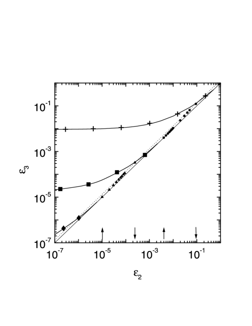
FIG. 2.: Trimer energies, $\epsilon_{3}$, as functions of the dimer bound state energy $\epsilon_{2}$. The trimer ground state energy ($\epsilon_{3}^{(0)}$) is shown by the curve with crosses; the first excited bound state ($\epsilon_{3}^{(1)}$) is shown by the curve with squares; and the second excited bound state ($\epsilon_{3}^{(2)}$) by the curve with diamonds. The behavior of two trimer virtual state energies, $\epsilon_{3v}^{(1)}$ (small circles) and $\epsilon_{3v}^{(2)}$ (small triangles) are also shown, as functions of the two-body energy, varying from the threshold $\epsilon_{3}=\epsilon_{2}$ (solid line) to the threshold for the one-particle-exchange cut $\epsilon_{3}=\frac{4}{3}\epsilon_{2}$ (dotted line). All the energies are given in arbitrary units.

The plot of Fig. 3 is constructed with the results for the first and second Thomas-Efimov states. This plot practically coincides with the corresponding one obtained from the second and third states (not shown). Figure 3 shows a universal route for the energy of the $(N+1)$ trimer state in the complex energy plane, from the second energy sheet to the first one as the ratio $E_{2}/E_{3}^{(N)}=\epsilon_{2}/\epsilon_{3}^{(N)}$ decreases. The three-body virtual state energy reaches $4E_{2}/3$ at $E_{2}/E_{3}^{(N)}=0.71$. Also realistic calculations for the helium-trimer are available and are displayed in this figure. The agreement between our calculations and the realistic ones, showns the power of our scaling picture. Unfortunately, there is not yet, to our knowledge realistic calculations of the virtual state in helium trimer or even in any other weakly bound three-boson system, in which our route should also applies. We emphasize that although we have presented results only for the second and third Thomas-Efimov states, the scaling limit is practically approached as we see in Fig. 3. We expect that going further in diminishing the absolute value of $E_{2}$ the new excited states will also follow the same route. The claim is of course that the route is universal for all states in the scaling limit.

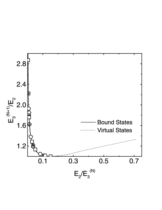
FIG. 3.: Ratio of the trimer excited or virtual $(N+1)-$th state energy as a function of the ratio of the dimer energy and trimer $N$-th bound state energy. The results for the trimer excited bound state energies are shown by the solid curve and the virtual state energies are shown by the dotted curves. Our calculations show that the results for $N=0$ and $N=1$ practically coincide. The symbols represent results from other calculations: empty squares ($s-$wave) and empty circles ($s+d$ waves) are from Ref. [30] (for $N=0$); crossed squares, from Ref. [31]; the crossed circle is from Ref. [32]; the triangle, from Ref. [33]; and the lozenge, from Ref. [34].

The results for the energy of the excited Efimov state in ⁴He₃ molecule given by ${\cal K}(z)$ ($z=[E_{2}/E_{3}^{(N)}]^{\frac{1}{2}}$), obtained by solving Eqs.(1), (11) and (15) in the scaling limit, are compared to the realistic model calculations also presented in Fig. 4. The homogeneous integral equation with the sharp cut-off momentum regulator, which generalizes Eq.(1) for the virtual trimer state is not written explicitly in the text as it can be easily derived. We observe the ratio $[({E^{(N+1)}_{3}}-E_{2})/{E^{(N)}_{3}}]^{\frac{1}{2}}$ depends on $z$ for realistic models, as well. In this plot we only show results for a bound dimer and $N=0$. The extreme limit of $z$ allowing the excited state are given by ${\cal K}(z)=0$ which gives $z=0.38$. The solution of Eqs.(1) and (11) in the scaling limit qualitatively reproduces the results for several interatomic potentials. A deviation is seen for $z\approx 0.4$ that are due to corrections from the finite range of the potential. The excited $(N+1)$ three-body state becomes virtual for $E_{2}/E_{3}^{(N)}>0.145$ (as seen in Fig. 3), implying that $E_{3}^{(N)}<6.9\;{\hbar^{2}}/{(ma^{2})}$ in this case. This threshold value agrees with the value previously found in Refs. [8, 9], recently confirmed in Ref. [35], for the condition of the disappearance of the excited trimer state in the limit of a zero-range interaction. Let us stress that the regularization schemes used in Eqs. (1) and (11) are consistent not only for the calculation of the bound excited trimer energies but also for the virtual trimer energies, as shown in Fig. 4. The small difference between the two regularization schemes tends to vanish fast for higher values of $N$.

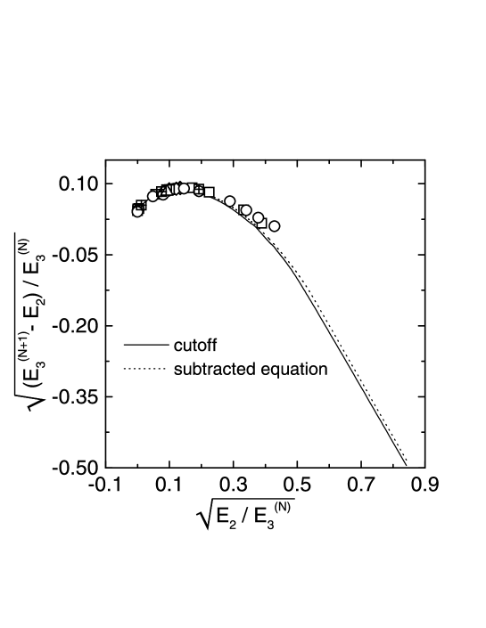
FIG. 4.: Results for the trimer bound and virtual excited $(N+1)-$th state energies, scaled by the $N-th$ bound-state energy. A comparison between calculations performed with cutoff and subtraction methods for the regularizations is given for $N=0$. We also present results from other calculations, as described in the caption of Fig. 3.

IV Conclusions

Natural scales determine the physics of quantum few-body systems with short-range interactions. The physical scales of three interacting particles, in the state of zero total angular momentum, are identified with the bound or virtual subsystems energy and the ground state three-body binding energy. The scaling limit is found when the ratio between the scattering length and the interaction range tends to infinity, while the ratio between the physical scales are kept fixed. This defines a scaling function for a given observable. From the formal point of view, we showed the relation of the scaling limit and the renormalization aspects of a few-body model with a zero-range interaction, through the derivation of subtracted three-body T-matrix equations, which are renormalization group invariant.

In the present work, we investigate the behavior of an excited Thomas-Efimov state as the binding energy of the subsystem increases with respect to the energy of the next lower bound three-body state. As shown, by allowing the two-body binding energy to increase in respect to the three-particle ground state energy, the excited three-body state disappears and a corresponding three-body virtual state emerges. The threshold for the three-body virtual state was found to be at the energy of the weakly bound trimer equal to $6.9\;{\hbar^{2}}/{(ma^{2})}$ for large positive scattering lengths $(a)$. The dependence of the $s-$wave virtual state three-body energy on the two and three atom ground state binding energies is calculated in the limit of a zero-range potential in a form of an universal scaling function. The scaling plots are an useful tool to classify observables and provide first guess to guide realistic calculations, as well as for planning experiments, with the aim of looking for weakly bound excited state of triatomic molecules.

The results of the present study can also be particularly relevant to the interpretation of experiments in atomic condensation, in which the effective atom-atom scattering length can be altered from negative to positive, in a wide range of values crossing zero-energy bound dimer [12]. For large positive scattering lengths, our estimate gives the threshold for the zero-binding trimer state, which allows to settle the experimental conditions for an investigation of the Efimov effect and search for their influence on the observables of condensed systems. On the other hand, large negative two-body scattering length have been recently investigated in Ref. [13]. There is the possibility that the observed discrepancy related with previous theoretical predictions can have their explanations in three-body effects, as well, because large two-body scattering lengths give the conditions where three-body (bound or virtual) Efimov states are likely to occur.

We would like to thank Fundação de Amparo à Pesquisa do Estado de São Paulo (FAPESP) and Conselho Nacional de Desenvolvimento Científico e Tecnológico (CNPq) for partial support.

REFERENCES

- [1] V. Efimov, Phys. Lett. B 33, 563 (1970) Nucl. Phys. A362, 45 (1981).
- [2] V. Efimov, Comm. Nucl. Part. Phys. 19, 271 (1990); and references therein.
- [3] D.V. Fedorov and A.S. Jensen, Phys. Rev. Lett. 71, 4103 (1993); D.V. Fedorov, A.S. Jensen and K. Riisager, Phys. Rev. Lett. 73, 2817 (1994); D.V. Fedorov, E. Garrido and A.S. Jensen, Phys. Rev. C51, 3052 (1995).
- [4] A. T. Stelbovics and L.R. Dodd, Phys. Lett. 39 B, 450 (1972); A.C. Antunes, V.L. Baltar and E.M. Ferreira, Nucl. Phys. A 265, 365 (1976).
- [5] S.K. Adhikari and L. Tomio, Phys. Rev. C26, 83 (1982); S.K. Adhikari, A.C. Fonseca and L.Tomio, Phys. Rev. C26, 77 (1982).
- [6] T.K. Lim, S.K. Duffy, and W.C. Damest, Phys. Rev. Lett. 38, 341 (1977); H.S. Huber, T.K. Lim and D.H. Feng, Phys. Rev. C 18, 1534 (1978).
- [7] A.E.A. Amorim, L. Tomio and T. Frederico, Phys. Rev. C46, 2224 (1992).
- [8] A.E.A. Amorim, T. Frederico and L. Tomio, Phys. Rev. C56, R2378 (1997).
- [9] T. Frederico, L. Tomio, A. Delfino, and A.E.A. Amorim, Phys. Rev. A60, R9 (1999).
- [10] A. Delfino, T. Frederico, L. Tomio, Few-Body Syst. 28, 259 (2000); J. Chem. Phys. 113, 7874 (2000).
- [11] M.H. Anderson, J.R. Ensher, M.R. Matthews, C.E. Wieman, E.A. Cornell, Science 269, 198 (1995); C.C. Bradley, C.A. Sackett, J.J. Tollett, and R.G. Hulet, Phys. Rev. Lett. 75, 1687 (1995); K.B. Davis, M.-O. Mewes, M.R. Andrews, N.J. van Druten, D.S. Durfee, D.M. Kurn, W. Ketterle, Phys. Rev. Lett. 75, 3969 (1995).
- [12] S. Inouye, M.R. Andrews, J. Stenger, H.-J. Miesner, D.M. Stamper-Kurn, W. Ketterle, Nature 392, 151 (1998); E. Timmermans, P. Tommasini, M. Hussein, and A. Kerman, Phys. Rep. 315, 199 (1999).
- [13] N.R. Claussen, E.A. Donley, S.T. Thompson, and C.E. Wieman, Phys. Rev. Lett. 89, 010401 (2002).
- [14] A. Gammal, T. Frederico, L. Tomio and Ph. Chomaz, J. of Phys. B 33, 4053 (2000); A. Gammal, T. Frederico, L. Tomio, and Ph. Chomaz, Phys. Rev. A 61, 051602 (2000); A. Gammal, T. Frederico, and L. Tomio, Phys. Rev. E 60, 2421 (1999).
- [15] E. Nielsen, D. V. Fedorov, A. S. Jensen, E. Garrido, Phys. Rep. 347, 373 (2001).
- [16] S. K. Adhikari, T.Frederico and I.D. Goldman, Phys. Rev. Lett. 74, 487 (1995); S.K. Adhikari and T. Frederico, Phys. Rev. Lett. 74, 4572(1995).
- [17] L.H. Thomas, Phys. Rev. 47, 903 (1935).
- [18] E.A. Kolganova and A.K. Motovilov, Phys. Atom. Nucl. 62, 1179 (1999).
- [19] T. Frederico, A. Delfino, L. Tomio, Phys. Lett. B 481, 143 (2000).
- [20] T. Frederico and H.-C. Pauli, Phys. Rev. D64: 054007 (2001); T. Frederico, A. Delfino, L. Tomio, V.S. Timóteo, Fixed Point Hamiltonians in Quantum Mechanics, hep-ph/01010165. T. Frederico, V.S. Timóteo, L. Tomio, Nucl. Phys. A 653, 209 (1999).
- [21] S.K. Adhikari, A. Delfino, T. Frederico, I. D. Goldman, L. Tomio, Phys. Rev. A37, 3666 (1988).
- [22] A.C. Fonseca, E.F. Redish, P.E. Shanley, Nucl. Phys. A 320, 273 (1979).
- [23] T. Frederico, I. D. Goldman, Phys. Rev. C36 R1661 (1987).
- [24] A. C. Phillips, Nucl. Phys. A 107, 109 (1968).
- [25] G.V. Skornyakov and K.A. Ter-Martirosian, Sov. Phys. JETP 4, 648 (1957).
- [26] W. Glöckle, Phys. Rev. C18, 564 (1978).
- [27] A. Delfino and T.Frederico, Phys. Rev. C53, 62 (1996).
- [28] A. Delfino, T. Frederico, M. S. Hussein, L. Tomio, Phys. Rev. C61, 051301(R) (2000).
- [29] T. Frederico, I.D. Goldman and A. Delfino, Phys. Rev. C 37, 497 (1988).
- [30] Th. Cornelius and W. Glöckle, J. Chem. Phys. 85, 3906 (1986).
- [31] S. Huber, Phys. Rev. A 31, 3981 (1985).
- [32] P. Barletta and A. Kievsky, Phys. Rev. A 64, 042514 (2001).
- [33] D.V. Fedorov, A.S. Jensen, J. Phys. A 34, 6003 (2001).
- [34] E.A. Kolganova, A.K. Motovilov, and S.A. Sofianos, Phys. Rev. A56, R1686 (1997).
- [35] E. Braaten, H.-W. Hammer, and M. Kusunoki, Universal Equation for Efimov States, arXiv:con-mat/0201281.