]http://bgaowww.physics.utoledo.edu

Effective potentials for atom-atom interaction at low temperatures

Abstract

We discuss the concept and design of effective atom-atom potentials that accurately describe any physical processes involving only states around the threshold. The existence of such potentials gives hope to a quantitative, and systematic, understanding of quantum few-atom and quantum many-atom systems at relatively low temperatures.

The concept of model potential has played an important role in many branches of physics. The well known examples include the Morse potential Morse (1929) and the Lennard-Jones potential for molecular systems, and the hard-sphere potential and the delta-function pseudopotential Huang and Yang (1957) widely used in many-body theories, including theories for Bose-Einstein condensates (BEC) Leggett (2001).

There are many reasons why one uses a model potential instead of the “real” potential. Here, we only emphasize that a problem can simply become unmanageable if the “real” potential is used. For quantum systems, this statement quickly becomes true for three or more atoms. This explains, in part, that despite its many limitations, it has proven difficult to go substantially beyond the Gross-Pitaveskii theory for BEC that is based on the delta-function pseudopotential Leggett (2001).

Our goal here is to discuss the concept and design of model potentials that better reflect the reality of atom-atom interaction than either the hard-sphere potential or the delta-function pseudopotential, yet simple enough to allow for applications in quantum few-atom and quantum many-atom systems. Here, being “simple”, to a large extent, means being shallow, as it is the depth of a potential, which can be measured by the number of bound states it supports, that determines the complexity of the resulting quantum few-atom and quantum many-atom problems.

One of our key conclusions is the following. For N-atom states around the N-atom threshold (such as the BEC state Leggett (2001)), or physical processes that involve only states around the threshold (such as the three-body recombination process Nielsen et al. (2001); Suno et al. (2002)), the interaction potential between a pair of atoms, no matter how deep it might be, can be replaced by an effective potential supporting only one or a few bound states. Furthermore, because different partial waves are described by the same effective potential, it can be used in precisely the same manner as any “real” potential. And in doing so, one reduces the complexity of the resulting quantum few-atom and quantum many-atom problems to a level comparable to that for He, a level that we are quickly learning to deal with Blume and Greene (2000); Suno et al. (2002).

If one thinks of the delta-function pseudopotential Huang and Yang (1957) as describing the atomic interaction at the longest length scale in the zero-energy limit, $2\pi/k$, the natural next step is the description of atomic interaction at the next, shorter, length scale. This scale is $\beta_{n}=(2\mu C_{n}/\hbar^{2})^{1/(n-2)}$, which characterizes the long-range atomic interaction of the form of $-C_{n}/r^{n}$ ($n>2$). The angular-momentum-insensitive quantum-defect theory (AQDT) Gao (2001, 2000) provides a systematic description of atom-atom interaction at this scale, and is the basis of our discussion.

Reference Gao (2001) focused on two-atom systems with $V(r)\rightarrow-C_{6}/r^{6}$, but the same concepts and formulation are readily generalized to any $n>2$. In this general formulation, a two-atom system with an asymptotic potential of the form of $-C_{n}/r^{n}$ ($n>2$) is described by a dimensionless K matrix $K^{c}(\epsilon,l)$ and a set of universal functions that are determined from the solutions of

$$\left[\frac{d^{2}}{dr^{2}}-\frac{l(l+1)}{r^{2}}+\frac{\beta_{n}^{n-2}}{r^{n}}+\bar{\epsilon}\right]u_{\epsilon l}(r)=0,$$ (1)

where $\bar{\epsilon}\equiv 2\mu\epsilon/\hbar^{2}$. Specifically, $K^{c}(\epsilon,l)$ is defined by writing the wave function at large distances as a linear superposition of a pair of reference solutions of Eq. (1):

$$u_{\epsilon l}(r)=A_{\epsilon l}[f^{c}_{\epsilon l}(r)-K^{c}(\epsilon,l)g^{c}_{\epsilon l}(r)]\;,$$ (2)

where $f^{c}$ and $g^{c}$ are purposely chosen to have the behavior

$$f^{c}_{\epsilon l} \stackrel{{\scriptstyle r\ll\beta_{n}}}{{\longrightarrow}} (2/\pi)^{1/2}(r/\beta_{n})^{n/4}\cos\left(y-\pi/4\right)\;,$$ (3)

$$g^{c}_{\epsilon l} \stackrel{{\scriptstyle r\ll\beta_{n}}}{{\longrightarrow}} -(2/\pi)^{1/2}(r/\beta_{n})^{n/4}\sin\left(y-\pi/4\right)\;,$$ (4)

for all energies Gao (2001). Here $y=[2/(n-2)](\beta_{n}/r)^{(n-2)/2}$.

AQDT asserts that $K^{c}(\epsilon,l)$ is approximately a constant that is independent of both $\epsilon$ and $l$, provided that $\beta_{n}$ is greater than other, energy-independent, length scales present in the system Gao (2001). For our purposes here, the most important conclusion of AQDT is the following. To the extent of $K^{c}(\epsilon,l)$ being energy and angular-momentum independent, potentials with the same type of long-range behavior (namely the same $n$) and the same $K^{c}$ have, on a scaled energy basis, the same bound spectra and scattering properties around the threshold Gao (2001). Here the bound spectra and scattering properties include all angular momentum states for which $K^{c}$ remains approximately $l$-independent.

Ignoring scaling relations implied by this statement, which will discussed elsewhere Gao , AQDT gives the following simple prescription for designing an effective potential that has the same physical properties around the threshold as the system of interest. First, choose a model potential. The only restriction is that it should have the right asymptotic behavior. Second, adjust the short range parameters of the model potential so that

$$K^{c}_{\rm mod}(0,l)=K^{c}(0,l)\;,$$ (5)

for one particular $l$. These two conditions do not uniquely determine an effective potential. Another auxiliary condition, which gives a convenient characterization of the depth of a potential, is the number of bound levels supported by a model potential for a particular $l$, $N_{l}$. For classes of model potentials discussed below, these conditions uniquely determine a model potential.

We stress here two classes of model potentials for which $K^{c}(0,l)$, and the number of bound levels for each $l$, $N_{l}$, can be found analytically. One class is of the type of a hard-sphere with an attractive tail:

$$V_{HST}(r)=\left\{\begin{array}[]{lcl}\infty&,&r\leq r_{0}\\ -C_{n}/r^{n}&,&r>r_{0}\end{array}\right.\;,$$ (6)

which will be denoted by HST. The other class is of the type of Lennard-Jones LJ$(n,2n-2)$:

$$V_{LJn}(r)=-C_{n}/r^{n}+C_{2n-2}/r^{2n-2}\;,$$ (7)

which will be denoted by LJn. In particular, this potential corresponds to a LJ(6,10) potential for $n=6$.

For HST potentials, it is not difficult to show that the $K^{c}$ parameter at zero energy is given by Gao

$$K_{\text{HST}}^{c}(0,l)=-\frac{J_{\nu_{0}}(y_{0})\cos(\pi\nu_{0}/2)-Y_{\nu_{0}}(y_{0})\sin(\pi\nu_{0}/2)}{J_{\nu_{0}}(y_{0})\sin(\pi\nu_{0}/2)+Y_{\nu_{0}}(y_{0})\cos(\pi\nu_{0}/2)},$$ (8)

where $\nu_{0}=(2l+1)/(n-2)$, $J$ and $Y$ are the Bessel functions Abramowitz and Stegun (1964), and $y_{0}=[2/(n-2)](\beta_{n}/r_{0})^{(n-2)/2}$. The number of bound levels for angular momentum $l$ is given by

$$N_{\text{HST}}(l)=\left\{\begin{array}[]{lcl}m&,&j_{\nu_{0},m}\leq y_{0}<j_{\nu_{0},m+1}\\ 0&,&y_{0}<j_{\nu_{0},1}\end{array}\right.\;,$$ (9)

where $j_{\nu_{0},m}$ ($m\geq 1$), is the m-th zero of the Bessel function $J_{\nu_{0}}(x)$ Abramowitz and Stegun (1964).

For LJn potentials, the following results can be derived with the help of a local scaling transformation Gao .

$$K_{\text{LJn}}^{c}(0,l)=\tan(\pi\nu_{0}/2)[1+h_{l}(z_{0})][1-h_{l}(z_{0})]^{-1},$$ (10)

where $z_{0}=(\beta_{n}/\beta_{2n-2})^{n-2}/[2(n-2)]$,

$$h_{l}(z_{0})=z_{0}^{\nu_{0}}\frac{\sin\pi(z_{0}+1/2-\nu_{0}/2)\Gamma(z_{0}+1/2-\nu_{0}/2)}{\sin\pi(z_{0}+1/2+\nu_{0}/2)\Gamma(z_{0}+1/2+\nu_{0}/2)},$$ (11)

and $\nu_{0}=(2l+1)/(n-2)$. The number of bound levels for any $l$ is given by

$$N_{\text{LJn}}(l)=\left\{\begin{array}[]{lcl}\left[z_{0}+\frac{1}{2}-\frac{\nu_{0}}{2}\right]&,&z_{0}\geq(\nu_{0}+1)/2\\ 0&,&z_{0}<(\nu_{0}+1)/2\end{array}\right.,$$ (12)

where $[x]$ means the greatest integer less than or equal to $x$. We note that scattering lengths, which are much more restrictive concepts Levy and Keller (1963); Gao (2000), can be derived from $K^{c}(0,l)$. For example, the $s$ wave scattering length, which is defined only for $n>3$, can be obtained from $K^{c}(0,l=0)$:

$$a_{l=0}/\beta_{n}=\left[b^{2b}\frac{\Gamma(1-b)}{\Gamma(1+b)}\right]\frac{K^{c}(0,0)+\tan(\pi b/2)}{K^{c}(0,0)-\tan(\pi b/2)}\;,$$ (13)

where $b=1/(n-2)$.

From these results, the HST and LJn types of potentials can be readily designed according to Eq. (5) to have the desired $K^{c}(0,l)$, and the desired $N_{l}$. Table 1 gives a selected set of designs for the triplet state of a ²³Na dimer. Here the potentials are designed to have $K^{c}(0,l=0)=13.57$, which is found numerically using the latest potential for a sodium dimer Laue et al. (2002). From Eq. (13), this corresponds to an $s$ wave scattering length of 64.57 a.u. The number of bound $s$ wave levels supported by this “real” potential is found numerically to be 16.

Table 1: Selected data, all in atomic units, for effective potentials designed for the triplet state of a ²³Na dimer. All potentials have $C_{6}=1556$ a.u. Derevianko et al. (1999) and $K^{c}(0,l=0)=13.57$. $N_{l=0}$ is the number of $s$ wave bound levels supported by the potential. $D_{e}$ is a derived parameter presented for discussion.

	LJ(6,10)		HST
$N_{l=0}$	$C_{10}$	$D_{e}$	$r_{0}$	$D_{e}$
1	1.65080e+9	2.64709e-7	3.22715e+1	1.37752e-6
2	4.05415e+8	2.17501e-6	2.40025e+1	8.13720e-6
4	1.00245e+8	1.76896e-5	1.74332e+1	5.54309e-5
16	6.21105e+6	1.14700e-3	8.89948e+0	3.13200e-3

Figure 1 shows the comparison of $s$ and $d$ wave partial cross sections of effective LJ(6,10) and effective HST potentials, both designed to support 16 $s$ wave bound levels and have a $K^{c}(0,l=0)=13.57$, with the Na-Na partial cross sections computed from the “real” potential Laue et al. (2002). The results are hardly distinguishable over a wide range of energies. In comparison, the hard-sphere potential (HS) fails quickly away from the threshold for the $s$ wave, and gives completely wrong results for the $d$ wave.

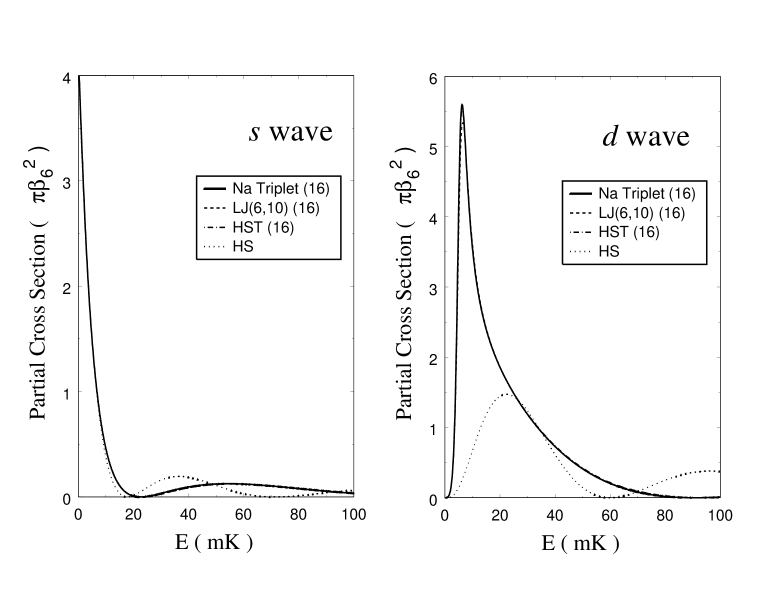
Figure 1: Comparison of $s$ and $d$ wave partial cross sections of effective LJ(6,10) and HST potentials, both designed to support sixteen $s$ wave bound levels and have $K^{c}(0,l=0)=13.57$, with the “real” Na-Na partial cross sections Na . The number in the parenthesis represents the number of $s$ wave bound levels supported by a potential. Results for a hard-sphere (HS) potential are also shown for comparison.

This result confirms the concept of effective potential based on AQDT. For our purposes here, however, what is more important is how shallow the effective potentials can be while still maintain a good description of low-energy characteristics of a real system. Figure 2 shows the comparison of $s$ and $d$ wave partial cross sections of an effective LJ(6,10) potential, in this case designed to support only a single $s$ wave bound state, with the “real” Na-Na results Na . The agreements remain excellent.

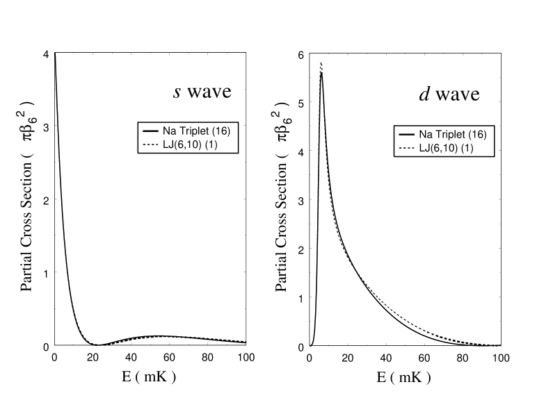
Figure 2: Comparison of $s$ and $d$ wave partial cross sections for an effective LJ(6,10) potential, designed to support a single $s$ wave bound level, with the “real” Na-Na cross sections Na .

Figure 3 shows similar results for a HST potential. In this case, the HST potential that supports only a single $s$ wave bound state does not do as well near the $d$ wave shape resonance. But it quickly improves, monotonically, as the number of bound levels it is designed to support increases. By $N_{l=0}=4$, a good agreement is achieved.

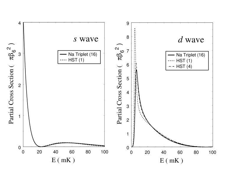
Figure 3: Comparison of $s$ and $d$ wave partial cross sections for effective HST potentials, designed to support one and four $s$ wave bound levels, with the “real” Na-Na cross sections Na .

The robustness of these designs is not limited to the description of scattering properties, it also applies to the energies of bound states that are close to the dissociation threshold, and to the wave functions. For example, for effective potentials supporting four $s$ wave bound levels, the HST gives a binding energy of 0.2027 GHz for the least-bound $s$ state, the LJ(6,10) gives 0.2003 GHz. Both in good agreement with the result for the “real” potential, which gives 0.2044 GHz Na . Figure 4 shows that for effective potentials supporting four $s$ wave bound levels, the wave functions are well represented down to $r=20$ a.u., covering basically all regions of space in which there is an appreciable amplitude.

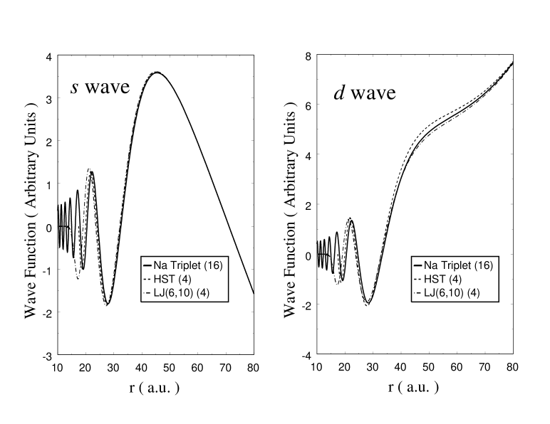
Figure 4: Zero-energy wave functions of effective potentials with four $s$ wave bound levels compared with the “real” Na-Na wave functions Na .

We stress that while only the results for sodium are presented here. They are used to illustrate much more general concepts. As the number of bound levels supported by an effective potential increases, all physical properties of states around the threshold converge to the same results (see Figs. 1-4). This is the shape-independence at length scale $\beta_{n}$. The converged results, properly scaled, represent a set of universal properties shared by all quantum systems with the same type of long-range potential, and characterized by the same, $l$-independent constant $K^{c}=\lim_{\beta_{x}/\beta_{n}\rightarrow 0}K^{c}(0,l)$ Gao (2001), where $\beta_{x}$ represent the next shorter length scale present in the system. The examples presented here, Figs. 2-4, show how quickly this set of universal properties are approached as one increases the number of bound levels supported by an effective potential. This quick convergence is due to the fact that deviations from the universal behavior depend on a high power of $\beta_{x}/\beta_{n}$ Gao . Other quantum systems differ from Na primarily in $K^{c}$ Gao (2001), which does not effect this rapid convergence.

Note that we did not make any distinction between two-atom and N-atom quantum systems in the statements above, because the same apply to a N-atom system. A short argument is simply that diffuse states, in which atoms are mostly at large distances relative to each other, only couple coherently to other diffuse states. A longer argument can proceed as follows. The correct $K^{c}(0,0)$, and therefore $a_{l=0}$, ensures the correct results at the mean-field level Leggett (2001). The correct two-atom wave function ensures the correct two-atom correlation. It also ensures the correct three-atom correlation, as follows. Think of a three-atom as a two-atom perturbed by another. Frank-Condon considerations tell one that only two-atom states around the threshold are significantly coupled. This means by having the correct two-atom wave functions around the threshold, one has also the correct three-atom correlation around the threshold. …

To illustrate the savings of computer resources as a result of using an effective potential, consider the problem of N interacting atoms in a symmetric trap of frequency $\omega$. If a real potential is used, the fact we need to represent the length scale of $(2\mu D_{e}/\hbar^{2})^{-1/2}$ means we need roughly $D_{e}/\hbar\omega$ number of harmonic oscillator states for each atom, for a total of $(D_{e}/\hbar\omega)^{N}$ number of states (ignoring statistics). If an effective potential is used, the corresponding number is $(D_{e,\text{eff}}/\hbar\omega)^{N}$. Thus the saving in the size of basis set is characterized by the factor $(D_{e,\text{eff}}/D_{e})^{N}$. For the triplet state of Na, $D_{e,\text{eff}}/D_{e}$ is of the order of $10^{-3}$ if an effective potential with two $s$ wave bound levels is used (see Table 1). This corresponds to a saving in the size of basis set of $10^{9}$ fold just for a three-atom problem. Even greater savings are achieved for deeper potentials or for more atoms. From another angle, for effective potentials with $N_{l=0}\sim 1$, all length scales shorter than $\beta_{n}$ have effectively been eliminated. It is this elimination of short length scales that makes a complex problem more manageable.

On the other hand, if a good description over an even wider range of energies around the threshold is desired, the same methodology can be carried to scales shorter than $\beta_{n}$ (e.g., $\beta_{8}$ for atoms with a $-C_{6}/r^{6}$ long-range interaction and a $-C_{8}/r^{8}$ correction) Gao . However, because the ratio $\beta_{8}/\beta_{6}$ is different for different systems, the results become dependent upon one more system-specific parameter. At this stage, going to shorter length scale seems useful only in specialized two-atom applications Gao . We also point out that it is around the threshold that the quantum effects are most important Gao (1999).

In conclusion, we have established the concept and design of effective potentials describing atomic interaction at the length scale of $\beta_{n}$. It is the scale that one has to deal with in studying quantum few-atom Nielsen et al. (2001) and quantum many-atom systems Leggett (2001) at finite temperature, of high density, or under strong confinement. We expect the method presented to play a role in our understanding of some of the more complex systems and processes at low temperatures, such as the three-body recombination process Nielsen et al. (2001); Suno et al. (2002), excited clusters states Blume and Greene (2000), and quantum liquids Leggett (2001). In all cases, one can look for, and verify universal properties at the scale of $\beta_{n}$, by comparing results from different designs, such as HST and LJn, and by checking convergences as one relaxes an effective potential towards more bound levels.