Spatiotemporal adaptation through corticothalamic loops: A hypothesis

Abstract

The thalamus is the major gate to the cortex and its control over cortical responses is well established. Cortical feedback to the thalamus is, in turn, the anatomically dominant input to relay cells, yet its influence on thalamic processing has been difficult to interpret. For an understanding of complex sensory processing, detailed concepts of the corticothalamic interplay need yet to be established. Drawing on various physiological and anatomical data, we elaborate the novel hypothesis that the visual cortex controls the spatiotemporal structure of cortical receptive fields via feedback to the lateral geniculate nucleus. Furthermore, we present and analyze a model of corticogeniculate loops that implements this control, and exhibit its ability of object segmentation by statistical motion analysis in the visual field.

Keywords: Lateral geniculate nucleus, Corticothalamic feedback, Control loop, Object segmentation, Motion analysis.
 
Published as Visual Neuroscience 17 (2000), pp. 107–118.  

Introduction

It has long been an intriguing problem that cortical feedback to the thalamus is the anatomically dominant input to relay cells, yet the modulation it effects in their responses seems to be ambiguous. Experiments and theoretical considerations have suggested a variety of operations of the visual cortex on the lateral geniculate nucleus (LGN), such as attention-related gating of geniculate relay cells (GRCs) [Sherman & Koch, 1986, Koch, 1987], synchronizing firing of GRCs [Sillito et al., 1994, Singer, 1994], increasing mutual information between GRCs’ retinal input and their output [McClurkin et al., 1994], and switching GRCs from a detection to an analyzing mode [Sherman & Guillery, 1996, Godwin et al., 1996]. Most of the current speculations, however, fall short of a clear, integrated view of corticothalamic function. Detailed concepts of the relationship between thalamic and cortical operation still remain to be established so as to advance our ideas about complex sensory, and ultimately cognitive, processing. In the present article we provide support for a role of corticogeniculate loops in complex visual motion processing.

In the A laminae of cat LGN two types of X relay cell have been identified that dramatically differ in their temporal response properties [Mastronarde, 1987a, Humphrey & Weller, 1988a, Saul & Humphrey, 1990]. Those that are more delayed in response time and phase have been termed lagged, the others nonlagged cells (with the exception of very few so-called partially lagged neurons). In particular, the peak response of lagged neurons to a moving bar is about 100 ms later than that of nonlagged neurons [Mastronarde, 1987a]. Lagged X cells comprise about 40 % of all X relay cells [Mastronarde, 1987a, Humphrey & Weller, 1988b]. Physiological [Mastronarde, 1987b], pharmacological [Heggelund & Hartveit, 1990], and structural [Humphrey & Weller, 1988b] evidence suggests that rapid feedforward inhibition via intrageniculate interneurons plays a decisive role in shaping the lagged cells’ response. Some authors have additionally related differences in receptor types to the lagged-nonlagged dichotomy [Heggelund & Hartveit, 1990, Hartveit & Heggelund, 1990]; see, however, Kwon et al. (1991).

Layer 4B in cortical area 17 of the cat is the target of both lagged and nonlagged geniculate X cells [Saul & Humphrey, 1992a, Jagadeesh et al., 1997, Murthy et al., 1998]. The spatiotemporal receptive fields (RFs) of its direction-selective simple cells can routinely be interpreted as being composed of subregions that receive geniculate inputs alternating between lagged and nonlagged X type [Saul & Humphrey, 1992a, Saul & Humphrey, 1992b, DeAngelis et al., 1995, Jagadeesh et al., 1997, Murthy et al., 1998]. At least for simple cells in layer 4B, this RF structure determines the response to moving visual features [McLean & Palmer, 1989, Reid et al., 1991, DeAngelis et al., 1995, Jagadeesh et al., 1993, Jagadeesh et al., 1997, Murthy et al., 1998], and thus the cell’s tuning for direction and speed.

Certainly, intracortical input to cortical cells contributes to direction-selective responses, given that these inputs anatomically outnumber thalamic inputs [Ahmed et al., 1994]. Suggested intracortical effects include sharpening of tuning properties by suppressive interactions [Reid et al., 1991, Hirsch et al., 1998, Crook et al., 1998] and amplification of geniculate inputs by recurrent excitation [Douglas et al., 1995, Suarez et al., 1995]. Intracortical circuits can in principle even generate their own direction selectivity by selectively inhibiting responses to nonpreferred motion [Douglas et al., 1995, Suarez et al., 1995, Maex & Orban, 1996]. Our modeling is complementary to the latter in that we emphasize the influence of geniculate inputs on cortical RF properties that is suggested by numerous studies [Saul & Humphrey, 1992a, Saul & Humphrey, 1992b, Reid & Alonso, 1995, Alonso et al., 1996, Ferster et al., 1996, Jagadeesh et al., 1997, Murthy et al., 1998, Hirsch et al., 1998], in order to bring out effects that are specific to the geniculate contribution to spatiotemporal tuning.

Thalamocortical neurons possess a characteristic blend of voltage-gated ion channels that jointly determine the timing and pattern of Na⁺ spiking in response to a sensory stimulus. Depending on the initial membrane polarization, the GRC response to a visual stimulus is in a range between a tonic and a burst mode [Sherman & Guillery, 1996]. At hyperpolarization, a Ca²⁺ conductance gets de-inactivated and, on activation, promotes burst firing. Although the issue is still controversial, there is evidence that a mixture of burst and tonic spikes is involved in the transmission of visual signals in lightly anesthetized or awake animals [Guido et al., 1992, Guido et al., 1995, Guido & Weyand, 1995, Mukherjee & Kaplan, 1995, Sherman & Guillery, 1996, Reinagel et al., 1999]. In nonlagged neurons a burst component is present at resting membrane potentials below roughly -70 mV and constitutes a very early part of a visual response [Lu et al., 1992, Guido et al., 1992, Mukherjee & Kaplan, 1995]. In lagged neurons bursting seems to be responsible for high-activity transients seen after the offset of feedforward inhibition; in particular, it is contributing substantially to the delayed peak response to a moving bar [Mastronarde, 1987b].

Cortical feedback to the A laminae of the LGN, arising mainly from layer 6 of area 17 [Sherman & Guillery, 1996], can locally modulate the response mode, and hence the timing, of GRCs by shifting their membrane potentials on a time scale that is long as compared to retinal inputs. This may occur directly through the action of metabotropic glutamate and NMDA receptors (depolarization) [McCormick & von Krosigk, 1992, Godwin et al., 1996, Sherman & Guillery, 1996] and indirectly via the perigeniculate nucleus (PGN) or geniculate interneurons by activation of GABA_B receptors (hyperpolarization) of GRCs [Crunelli & Leresche, 1991, Sherman & Guillery, 1996]. Indeed, GRCs in vivo are dynamic and differ individually in their degree of burstiness [Lu et al., 1992, Guido et al., 1992, Mukherjee & Kaplan, 1995]. Here we explicate the causal link between the variable response timing of GRCs and variable tuning of cortical simple cells for speed of moving features, thus identifying control of speed tuning as a likely mode of corticothalamic operation. Moreover, we exemplify the computational power of the hypothesized control mechanism in a model of corticogeniculate loops that performs object segmentation based on motion cues.

Geniculate input to the cortex

The first object of our study is the geniculate input to a cortical neuron in layer 4B.

Model of the primary visual pathway

For the GRCs we have employed a 12-channel model of the cat relay neuron [Huguenard & McCormick, 1992, McCormick & Huguenard, 1992], adapted to 37 degrees Celsius. It includes a transient and a persistent Na⁺ current, several voltage-gated K⁺ currents, a voltage- and Ca²⁺-gated K⁺ current, a low- and a high-threshold Ca²⁺ current, a hyperpolarization-activated mixed cation current, and Na⁺ and K⁺ leak conductances. As shown in Fig. 1a, retinal input reaches a GRC directly as excitation, and indirectly via an intrageniculate interneuron as inhibition, thus establishing the typical triadic synaptic circuit found in the glomeruli of X GRCs [Sherman & Guillery, 1996]. The temporal difference between the two afferent pathways equals the delay of the inhibitory synapse and has been taken to be 1.0 ms [Mastronarde, 1987b].

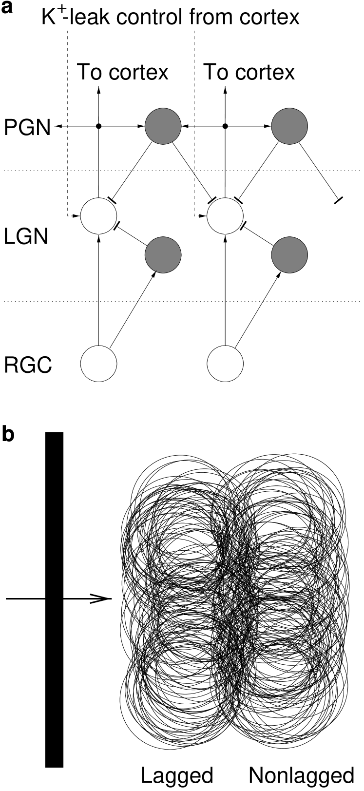
Figure 1: Model of the primary visual pathway. (a) Sketch of the lateral geniculate nucleus (LGN). Open/filled circles and arrow/bar heads indicate excitatory/inhibitory neurons and their respective synapses. A retinal ganglion cell (RGC) synapses excitatorily on a geniculate relay cell (GRC) and on an intrageniculate interneuron, which in turn inhibits the same GRC (arrangement called ‘synaptic triad’). The relative strengths of feedforward excitation and feedforward inhibition shape a GRC’s response to be of the lagged or nonlagged type; see main text and Fig. 2. There is an inhibitory feedback loop via the perigeniculate nucleus (PGN). The influence of cortical feedback has been modeled as a variation of the GRCs’ resting membrane potential by control of a K⁺ leak current. (b) Arrangement in visual space of the receptive field (RF) centers of the 100 lagged and 100 nonlagged GRCs comprising the model LGN. These GRCs are envisaged to project onto the same cortical simple cell and create an on or off region of its RF. In the simulations, the diameter of a single lagged or nonlagged RF center is 0.5 degrees. Results for rescaled versions of this geometry can be derived straightforwardly from the simulations; see main text. The bar and arrow on the left indicate preferred orientation and direction of motion, respectively.

It is known that both NMDA and non-NMDA receptors contribute to retinogeniculate excitation to varying degrees, ranging from almost pure non-NMDA to almost pure NMDA mediated responses in individual GRCs of both lagged and nonlagged varieties [Kwon et al., 1991]. At least in lagged cells, however, early responses and, hence, responses to the transient stimuli that will be considered here, seem to depend to a lesser degree on the NMDA receptor type than late responses [Kwon et al., 1991]. Since the essential characteristics of lagged and nonlagged responses apparently do not depend on the special properties of NMDA receptors – an assumption confirmed by our results – we chose the postsynaptic conductances in GRCs to be of the non-NMDA type.

The time course of postsynaptic conductance change in GRCs following reception of an input has been modeled by an alpha function,

$${\rm g}(t>0)\,=\,g_{\rm syn}\,\frac{t}{\tau_{\rm syn}}\,\exp\!\left(1-\frac{t}{\tau_{\rm syn}}\right)\ .$$ (1)

For excitation, the rise time $\tau_{\rm syn}$ has been chosen to be 0.4 ms [Mukherjee & Kaplan, 1995], for inhibition it is 0.8 ms. The latter value was estimated from the relative durations of S potentials recorded at excitatory and inhibitory geniculate synapses [Mastronarde, 1987b] and was found to reproduce the rise times of inhibitory postsynaptic potentials recorded in relay cells following stimulation of the optic chiasm [Bloomfield & Sherman, 1988]. The reversal potentials are for excitation 0 mV, for inhibition $-$85.8 mV [Bal et al., 1995].

We have found typical lagged responses for strong feedforward inhibition with weak feedforward excitation, in agreement with Mastronarde (1987b), Humphrey & Weller (1988b), and Heggelund & Hartveit (1990). On the other hand, typical nonlagged responses are produced by weak feedforward inhibition with strong feedforward excitation; see Fig. 2. We have therefore implemented lagged and nonlagged relay cells in the model by varying the relative strengths of feedforward excitation and feedforward inhibition. For an explanation of lagged and nonlagged responses see the results below.

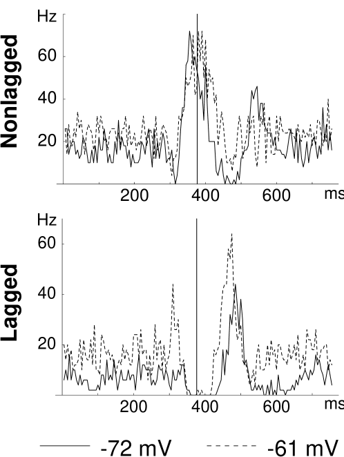
Figure 2: Numerical simulation of moving-bar response of single relay neurons. Typical nonlagged (top row) and lagged (bottom row) responses to a bar moving at 4 deg/s (100 sweeps averaged, bin width 5 ms) have been reproduced by relay neurons in the LGN model (Fig. 1a) at the two resting membrane potentials $-$61 mV (dashed line) and $-$72 mV (solid line). The vertical line in the center of the plots indicates the time of the retinal input peak. As the membrane is hyperpolarized, the nonlagged bar-response peak shifts to earlier times. Conversely, the lagged response shifts to later times. The nonlagged responses are produced by strong feedforward excitation [$g_{\rm syn}=0.05\mu$S; cf. eqn. (1)] and weak feedforward inhibition ($g_{\rm syn}=0.0125\mu$S), whereas the lagged responses correspond to weak feedforward excitation ($g_{\rm syn}=0.0125\mu$S) and strong feedforward inhibition ($g_{\rm syn}=0.25\mu$S). The numerical values of $g_{\rm syn}$ are not critical. The response timing is consistent with experiments [Mastronarde, 1987a, Lu et al., 1992, Guido et al., 1992]. Furthermore, we have found the temporal transfer functions (not shown) to agree well with published data [Saul & Humphrey, 1990, Mukherjee & Kaplan, 1995].

The model system comprises 100 lagged and 100 nonlagged relay neurons. Their RF centers are 0.5 degrees in diameter [Cleland et al., 1979] and are spatially arranged in a lagged and a nonlagged clusters subtending 0.7 degrees each and displaced by 0.45 degrees; see Fig. 1b. This layout matches the basic structure of an on or off region in a RF of a directional simple cell in cortical layer 4B onto which the GRCs are envisaged to project [Saul & Humphrey, 1992a, Saul & Humphrey, 1992b, DeAngelis et al., 1995, Jagadeesh et al., 1997, Murthy et al., 1998]. To complete the geniculate input to a RF of this type, this lagged-nonlagged unit would have to be repeated with alternating on-off polarity and a spatial offset that would determine the simple cell’s preference for some spatial frequency. Since we are not concerned here with effects of spatial frequency (see previous footnote 1), omission of the other on/off regions does not affect our conclusions. Results for rescaled RF geometries can be derived straightforwardly; see the results below. The number of geniculate cells contributing to the simple cell’s RF has been estimated roughly from Ahmed et al. (1994). Only its order of magnitude matters.

We have also taken into account feedback inhibition via the PGN [Lo & Sherman, 1994, Sherman & Guillery, 1996]; see Fig. 1a. Connections between PGN neurons and GRCs are all to all within, and separate for the lagged and nonlagged populations. Axonal plus synaptic delays are 2.0 ms in both directions.

Intrageniculate interneurons and PGN cells, like GRCs, posses a complex blend of ionic currents. They are, however, thought to be active mainly in a tonic spiking mode during the awake state [Contreras et al., 1993, Pape et al., 1994]. For an efficient usage of computational resources and time we have therefore modeled these neurons by the spike-response model [Gerstner & van Hemmen, 1992], which gives a reasonable approximation to tonic spiking [Kistler et al., 1997]. Note that for the present model it is irrelevant whether transmission across dendrodendritic synapses between intrageniculate interneurons and GRCs actually occurs with or without spikes; cf. Cox et al. (1998). For a relay neuron, all that matters is the fact that an excitatory retinal input is mostly followed by an inhibitory input [Bloomfield & Sherman, 1988]. The spike-response neurons have been given an adaptive spike output [Gerstner & van Hemmen, 1992], i.e., there is adaptation of transmission across the dendrodendritic synapses.

We have incorporated the influence of cortical feedback to the thalamus by varying the K⁺ leak conductivity of GRCs, which in turn controls their resting membrane potential [McCormick & von Krosigk, 1992, Godwin et al., 1996]; see Fig. 1a. All GRCs, lagged and nonlagged, have been assigned the same resting membrane potential; here we assume a uniform action of cortical feedback on the scale of single RFs in area 17. By varying the resting membrane potential we investigate a strictly modulatory role of corticogeniculate feedback, as opposed to the retinal inputs that drive relay cells to fire; cf. Sherman & Guillery (1996), Crick & Koch (1998).

The model is described by a high-dimensional system of nonlinear, coupled differential equations [Huguenard & McCormick, 1992, McCormick & Huguenard, 1992]. The input to GRCs was modeled as a set of Poisson spike trains with time-varying firing rates as recorded from retinal ganglion cells in response to moving, thin (0.1 degrees), long (10 degrees) bars [Cleland & Harding, 1983]. For numerical integration of the stochastic differential equations we used an adaptive fifth-order Runge-Kutta algorithm. The dynamics of spike-response neurons has been solved by exact integrals. Simulations were run on an IBM SP2 parallel computer.

We collected spike times with 0.1 ms resolution. For each velocity $v$ of bar motion tested, spikes of all 100 lagged/nonlagged relay cells were pooled. We calculated the total lagged/nonlagged response rates ${\rm r}_{\rm l}(v,t)$/${\rm r}_{\rm nl}(v,t)$ as spike counts in 5 ms windows, a timescale relevant to postsynaptic integration, shifted by steps of 1 ms, i.e., $t=1,2,\ldots$ ms. The velocity tuning of the pooled lagged/nonlagged peak rate per neuron is

$${\rm R}_{\ell}(v)\,=\,\frac{1}{100}\,\max_{t\in[t_{\rm i},t_{\rm f}]}{\rm r}_{\ell}(v,t)\ ,\quad\ell={\rm l},{\rm nl}\ ,$$ (2)

where the times $t_{\rm i}$ and $t_{\rm f}$ are chosen such that all responses lie in the interval $[t_{\rm i},t_{\rm f}]$.

We are primarily interested in the total geniculate input to a cortical simple cell. To this end, we have shifted lagged spikes by 2 ms to later times in order to account for the fact that the lagged cells’ conduction times to cortex are slightly longer than those of the nonlagged cells [Mastronarde, 1987a, Humphrey & Weller, 1988a]. Furthermore, although lagged responses in the LGN tend to be weaker than nonlagged responses [Mastronarde, 1987a, Humphrey & Weller, 1988a, Saul & Humphrey, 1990], they appear to be about equally effective in driving cortical simple cells [Saul & Humphrey, 1992a]. The cortical (possibly synaptic) cause being beyond the scope of this work, we simply have counted every lagged spike twice to obtain the velocity tuning of the effective geniculate input to a cortical cell,

$${\rm R}(v)\,=\,\frac{1}{100}\,\max_{t\in[t_{\rm i},t_{\rm f}]}\left[2\,{\rm r}_{\rm l}(v,t-2\,{\rm ms})+{\rm r}_{\rm nl}(v,t)\right]\ .$$ (3)

The peak input rate per lagged-nonlagged pair ${\rm R}(v)$ is correlated with simple-cell activity because postsynaptic potentials are summed almost linearly in simple cells [Jagadeesh et al., 1993, Kontsevich, 1995, Jagadeesh et al., 1997].

The total geniculate input rate to a cortical neuron depends on (i) the magnitude of the pooled lagged and nonlagged response peaks, ${\rm R}_{\rm l}(v)$ and ${\rm R}_{\rm nl}(v)$, respectively, and (ii) their relative timing. To differentiate between these two factors we have determined the times ${\rm t}_{\rm l}(v)$ and ${\rm t}_{\rm nl}(v)$ of the maxima of the lagged and nonlagged response rates, respectively,

$${\rm t}_{\ell}(v)\,=\,{\rm arg}\max_{t\in[t_{\rm i},t_{\rm f}]}{\rm r}_{\ell}(v,t)\ ,\quad\ell={\rm l},{\rm nl}\ ,$$ (4)

and calculated the peak-time differences ${\rm t}_{\rm nl}(v)-{\rm t}_{\rm l}(v)$ as a function of the bar velocity. Means and standard errors have been estimated from a sample of 30 sweeps at each bar velocity.

Results for geniculate input to the cortex

For different values of the resting membrane potential, Fig. 3 shows in the columns from left to right the velocity tuning of the lagged population (${\rm R}_{\rm l}$), of the nonlagged population (${\rm R}_{\rm nl}$), the peak-time differences (${\rm t}_{\rm nl}-{\rm t}_{\rm l}$) of their responses for the preferred direction, and the tuning of the total geniculate input (R) to a cortical cell for the preferred and nonpreferred direction of motion; see above for details. As in vivo, the lagged cells prefer lower velocities and have lower peak firing rates than the nonlagged cells [Mastronarde, 1987a, Humphrey & Weller, 1988a, Saul & Humphrey, 1990]. The key observation, however, is that the maximum of the total geniculate input rate to a cortical neuron shifts to lower velocities as the membrane potential hyperpolarizes; see Fig. 3 right column.

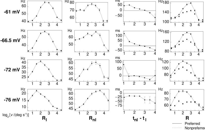
Figure 3: Numerical simulation of geniculate moving-bar response and input to cortex. Velocity tuning and timing of the response peaks have been plotted for resting membrane potentials indicated on the far left. In the columns we show from left to right as functions of the bar velocity the peak response rate of the lagged population (${\rm R}_{\rm l}$), of the nonlagged population (${\rm R}_{\rm nl}$), their peak-time difference (${\rm t}_{\rm nl}-{\rm t}_{\rm l}$) for the preferred direction, and the peak of the total geniculate input (R) to a cortical cell for the preferred (solid line) and nonpreferred (dotted line) direction of motion. The horizontal axes show the logarithm (base 2) of speed in all graphs. The bars in the graphs are standard errors. As the membrane is hyperpolarized, the total geniculate input to a cortical cell, and hence that cortical cell, prefer progressively lower velocities. Means and standard errors are estimated from 30 bar sweeps.

The total geniculate input rate R assumes its maximum at a velocity of bar motion where the peak discharges of the lagged and nonlagged neurons coincide, i.e., where ${\rm t}_{\rm nl}-{\rm t}_{\rm l}\approx 0$. The shift of the maximum with hyperpolarization to lower velocities is produced by a corresponding shift of the peak-time differences ${\rm t}_{\rm nl}-{\rm t}_{\rm l}$ and of the lagged tuning ${\rm R}_{\rm l}$, while the peak of the nonlagged tuning ${\rm R}_{\rm nl}$ remains essentially unchanged. As is demonstrated in Fig. 2, the change in peak-time difference is due to (i) a shift of the lagged response peak to later times, and (ii) a shift of the nonlagged response peak to earlier times.

The reason for the opposite shifts of lagged and nonlagged response timing lies in the interaction of the low-threshold Ca²⁺ current with the different levels of inhibition received by lagged and nonlagged neurons. With only weak feedforward inhibition, nonlagged neurons respond to retinal input with immediate depolarization, eventually reaching the activation threshold for the Ca²⁺ current. If the Ca²⁺ current is in the de-inactivated state, it will boost depolarization and give rise to an early burst component of the visual response [Lu et al., 1992, Guido et al., 1992]. The lower the resting membrane potential, the more de-inactivated the Ca²⁺ current will be, and the stronger the early response component relative to the late tonic component. In an ensemble of neurons that receive retinal input at slightly different times, like the 100 nonlagged neurons with spatially scattered RFs (cf. Fig. 1b), this leads to a gradual shift of the ensemble-response maximum with membrane polarization. Lagged neurons, on the other hand, receive strong feedforward inhibition and, hence, initially respond to retinal input with hyperpolarization. Repolarization occurs when inhibition gets weaker due to declining retinal input rate or adaptation of the inhibitory input. With the Ca²⁺ current being de-inactivated by the excursion of the membrane potential to low values, lagged spiking starts with burst spikes as soon as the voltage reaches the Ca²⁺-activation threshold. This will take longer, if the resting membrane potential is lower, leading to the observed shift in response timing with membrane polarization.

Not surprisingly, the total geniculate input rate R is higher for the direction of bar motion where ${\rm t}_{\rm nl}-{\rm t}_{\rm l}$ assumes lower values. In other words, the direction preferred is the one where the lagged cells receive their retinal input before the nonlagged cells; cf. Figs. 1b and 3 right column.

We have investigated the geniculate input to simple cells, which clearly cannot be compared with their output directly. Nonetheless it is interesting to note that, much like velocity tuning in areas 17 and 18 [Orban et al., 1981], the modeled geniculate input at the optimal velocity decreases and the tuning width increases with decreasing optimal velocity; see Fig. 3 right column.

Because of scaling properties of the retinal ganglion cells’ velocity tuning [Cleland & Harding, 1983], rescaled versions of the RF geometry shown in Fig. 1b produce accordingly shifted tuning curves (on a logarithmic speed scale). In particular, we retrieve the positive correlation between RF size and preferred speed found in areas 17 and 18 [Orban et al., 1981] from the geniculate input.

The corticogeniculate loop

Once a dynamic gating mechanism for thalamocortical information transfer has been identified, one has to face the key question of how gating can be controlled. The computational goal of this control should certainly be an enhanced cortical representation of behaviorally relevant stimuli, generally referred to as objects, and suppression of less significant bits, such as neuronal noise and incoherent background motion. The general idea of object segmentation by adaptive velocity tuning is illustrated in Fig. 4. Since many details of corticothalamic circuits are not known yet and since we aim at a thorough analytical treatment of the closed-loop system for general stimulus statistics we have kept the modeling at this point at a more abstract level than in the above case. Moreover, the underlying principles are best exposed by a simple model.

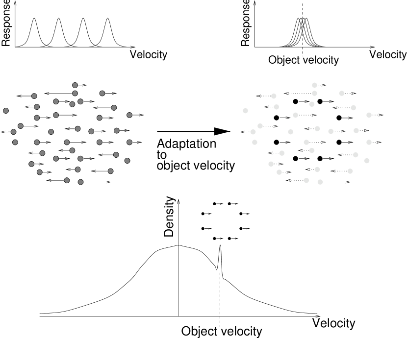
Figure 4: The rationale of object segmentation by adaptive velocity tuning. The tuning curves shown at the top of the figure schematically represent the peak response rates of (four) cortical neurons as a function of the speed of a local feature passing their receptive field in an unadapted state (top left) and an adapted state (top right). Within some region of the visual field a natural stimulus consists of a collection of local features (depicted as dots, center) moving from left to right and from right to left at various speeds (depicted as arrows). A subset of them is moving at a common speed from left to right. The velocity density (bottom) of this type of stimulus consists of two components: one symmetrical with respect to the two directions of motion and one asymmetrical. The former derives from the incoherent, the latter from the coherent motion and is the statistical signature of a moving object. The adaptive motion system has to detect and tune in to the asymmetrical component of the velocity density. After adaptation of cortical velocity tuning (top right), object features are prominent in cortical representation, whereas other features are suppressed (center right). The given stimulus scenario generalizes straightforwardly to motion in two dimensions.

Model of the corticogeniculate loop

The membrane potential of GRCs is assumed to be modulated by feedback from cortical layer 6. The postsynaptic potential evoked in GRCs by a burst of layer 6 action potentials fired around time $t_{i}$ is

$${\rm PSP}(t-t_{i})\,=\,\frac{t-t_{i}}{\tau}\,\exp\!\left(1-\frac{t-t_{i}}{\tau}\right)\ ,\quad\mbox{($t>t_{i}$),}$$ (5)

that is, an alpha function. We are interested here specifically in the slow, modulatory effect of cortical input, mediated by NMDA and metabotropic glutamate receptors in the case of depolarization, and by GABA_B receptors for hyperpolarization. The rise time $\tau$ for combinations of NMDA and metabotropic glutamate receptor responses and for GABA_B receptor responses may be several 100 ms [von Krosigk et al., 1999], but is kept as a free parameter in the model, i.e., we do not specify a numerical value for $\tau$ throughout the analysis. We neglect corticothalamic delays, which are at least one order of magnitude smaller than $\tau$. In particular, for layer 6 projection neurons that are visually responsive and thus relevant to our model, they are mostly below 10 ms [Tsumoto et al., 1978, Tsumoto & Suda, 1980]. One can show that the inclusion of an adequate distribution of delays does not alter the general dynamic behavior of the system, but merely adds small corrections to some characteristic quantities.

As illustrated by Fig. 4, cortical feedback signals that carry information on local velocity measurements need to be sampled from an extended visual field, spanning several RFs of cells in the primary visual cortex. Lateral spread of information may be implemented either by intracortical connections, or by divergence in the corticogeniculate feedback pathway; cf. Fig. 5 right. Let us label all events of cortical responses to local features within the entire population of layer 6 neurons that feed back onto GRCs by an index $i$ according to their temporal order, i.e., $t_{1}<t_{2}<\ldots$. Let furthermore ${\rm N}(t)$ be the number of such events until time $t$. The slow dynamics of a GRC’s membrane potential under cortical control then is

$$V(t)\,=\,\sum_{i=1}^{{\rm N}(t)}A_{i}\,{\rm PSP}(t-t_{i})+V_{0}\ ,$$ (6)

where $A_{i}$ is the amplitude of the $i$th event of cortical feedback that depends on the firing rate of a layer 6 neuron at time $t_{i}$. In this formulation the size of the layer 6 population in the adaptive system, and hence of the visual field from which motion information is integrated, is represented by the number of response events per time: the rate of events increases with the area from which motion is sampled.

Superimposed on the slow, cortically controlled dynamics [eqn. (6)] of GRCs’ membrane potentials is the relatively fast dynamics triggered by retinal input. The retinal input and its consequences have been the subject of study above. In the present model the dynamics of retinal input will not enter explicitly. Instead, we now care only for its cortical effect, that is, for cortical velocity tuning.

Cortical response rates in layer 4 to moving visual features such as bars are assumed to follow some kind of velocity-tuning function. We have demonstrated above that the velocity that produces the maximal convergent input from lagged and nonlagged geniculate relay cells is, not surprisingly, close to the velocity that yields coincident lagged and nonlagged response peaks, corresponding to ${\rm t}_{\rm nl}(v)-{\rm t}_{\rm l}(v)\approx 0$; cf. Fig. 3 third column. In this spirit we define a layer 4 cell’s response rate to a feature moving with velocity $v$ into the cell’s preferred direction as

$$R\,=\,{\rm f}\left[|{\rm t}_{\rm nl}(v)-{\rm t}_{\rm l}(v)|\right]\ ,$$ (7)

where f is some positive, monotonically decreasing function. For analytical treatment there will be some further restriction on f, to be formulated below. Moreover, we assume layer 4 cells not to respond to features moving in their null direction.

By looking at Fig. 3 third column, we see that the simulation data are roughly consistent with

$$\left[{\rm t}_{\rm nl}-{\rm t}_{\rm l}\right](v,V)\,=\,{\rm s}(v)-{\rm c}(V)\ ,$$ (8)

where s and c are monotonically decreasing functions of the stimulus velocity $v$ and the relay cells’ membrane potential $V$, respectively. This approximation seems to be better at higher membrane potentials. Velocity tuning is thus given by

$$R\,=\,{\rm f}\left[|{\rm s}(v)-{\rm c}(V)|\right]\ .$$ (9)

Note that this family of functions is rather general in that it fits a large set of velocity-tuning characteristics.

To obtain a physical interpretation of ${\rm s}(v)$ and ${\rm c}(V)$, we note that the naive understanding of the velocity-dependence of ${\rm t}_{\rm nl}(v)-{\rm t}_{\rm l}(v)$ is that it arises from the visual feature crossing the lagged-nonlagged compound RF (see Fig. 1b) in a time proportional to $1/v$. Rewriting eqn. (8) as

$${\rm c}(V)\,=\,{\rm t}_{\rm l}-({\rm t}_{\rm nl}-{\rm s})\ ,$$ (10)

it is evident that if s is the time it takes the visual feature to travel from the lagged RFs to the nonlagged RFs, c is the difference in response times intrinsic to the lagged and nonlagged populations. Appealing to this interpretation, we will write

$$s_{i}:={\rm s}(v_{i})\ ,\quad{\rm RTD}(t):={\rm c}[V(t)]\ ,\quad R_{i}:={\rm f}\left[|s_{i}-{\rm RTD}(t_{i})|\right]\ ,$$ (11)

and refer to $s_{i}$ as the stimulus passage time and to ${\rm RTD}(t)$ as the (dynamic) response time difference between the lagged and nonlagged populations. As above, the index $i$ enumerates the cortical response events in temporal order. The response of a layer 4 neuron is thus maximal, if the stimulus passage time equals the lagged-nonlagged response time difference.

We will use the simplest approximation for the dependence of the response time difference on the membrane potential,

$${\rm RTD}(t)\,=\,\chi V(t)+{\rm RTD}_{0}\ ,$$ (12)

that is, a linear function of $V$ with slope $\chi$ and offset ${\rm RTD}_{0}$.

In order to close the corticogeniculate loop, and the system of equations, we need a transformation of the layer 4 responses $R_{i}$ to the feedback signals of layer 6 cells, which in turn determine the amplitudes of postsynaptic potentials $A_{i}$ in GRCs. To this end, we have analyzed a simple implementation of cortical control. The rationale is that each cortical response $R_{i}$ to a stimulus $s_{i}$ triggers a postsynaptic potential of amplitude $A_{i}$ through feedback, either directly (depolarization, $A_{i}>0$), or via the PGN or geniculate interneurons (hyperpolarization, $A_{i}<0$), such that the response time difference ${\rm RTD}(t)$ is pulled closer to the stimulus passage time $s_{i}$.

For the computation of the feedback signal a layer 4 cell’s response activity serves as a measure of the amount of mismatch between ${\rm RTD}(t_{i})$ and $s_{i}$: low activity indicates large mismatch, high activity signals a good match [cf. eqn. (9)]. The sign of mismatch is computed by comparing the outputs of layer 4 cells preferring the same direction but different speeds, corresponding to different values of $V_{0}$ in eqn. (6). A simple network of spike-response neurons, shown in Fig. 5 left, approximates these principles and provides the corresponding feedback signals to the LGN. More precisely, computer simulations of this network show that

$$A_{i}\,\approx\,\gamma\,{\rm A}(R_{i})\,\sigma(R^{>}_{i}-R^{<}_{i})\ ,$$ (13)

where A is some positive, monotonically decreasing function, $\sigma$ is a sigmoidal function running between $-1$ and $+1$, and $R^{>}_{i}$, $R^{<}_{i}$ are response rates of layer 4 cells tuned to higher and lower speeds than the cell producing the response $R_{i}$. The factor $\gamma$ describes the overall strength of cortical feedback to the LGN. Eqn. (13) is the relation we used between layer 4 responses and amplitudes of GRC potentials. Note that it is the result of a simple transformation of the layer 4 activity to the feedback signals of layer 6 cells; cf. Fig. 5 left. Although a LGN-layer-4-layer-6-LGN loop of synaptic connections is indeed supported by anatomical data [Katz, 1987, Sherman & Guillery, 1996], our aim was primarily to investigate a network as simple as possible that can do the necessary computation.

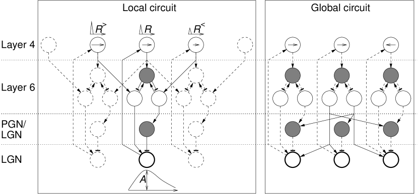
Figure 5: Model of corticogeniculate loop. Same conventions as in Fig. 1a. The thick circles symbolize all geniculate relay cells (GRCs), lagged and nonlagged, which project to a particular cortical layer 4 cell (cf. Fig. 1b), as indicated by the long upward arrows. On the left we show a local piece of circuit (Local circuit). The cells depicted here in layer 4 have coinciding receptive fields, the same preferred direction but different preferred speed of motion, as indicated by the arrows of different length (a longer arrow means a higher preferred speed). The temporal responses of these cells to a moving feature have different rate amplitudes (top; amplitudes $R^{>}$, $R$, $R^{<}$). Cortical feedback to the lateral geniculate nucleus (LGN), originating from layer 6, modulates the membrane potential of GRCs. Direct feedback depolarizes, indirect feedback via the perigeniculate nucleus (PGN) or geniculate interneurons hyperpolarizes the membrane of relay cells. The net effect is a slow postsynaptic potential of amplitude $A$ in GRCs (bottom). Simulation of the local circuit shows that $A$ is well-described by eqn. (13). The dashed parts of the local circuit indicate the analogous connections that feed back to GRCs which provide input to the other local layer 4 neurons. At the right of the figure we sketch the global, or long-range, connectivity of the system (Global circuit). The local circuit, shown here only for one speed-tuned layer 4 neuron, is replicated for different retinal positions and two opposite directions of motion (arrows). Local circuits with identical speed tuning in layer 4 are globally interconnected by divergence in the feedback pathway. Excitatory and inhibitory inputs to the GRCs are interchanged for feedback from cortical neurons with opposite direction preferences, as indicated once for each type of feedback connection by the solid arrows. Because of the long-range connections, each GRC receives modulatory input from cortical cells jointly representing an extended visual field, with antagonism between the two direction populations. Note that, rather than by divergence in the corticogeniculate projection, the same function could alternatively be implemented by lateral intracortical connections.

For the above control mechanism to work, sets of cortical layer 4 neurons are required that have overlapping RFs and differ in speed tuning. It is not necessary, but conceptually most straightforward, to assume the same set of $n$ classes of neurons, defined by the initial values $V_{0}^{(c)}$ [cf. eqn. (6)], $c=1,2,\ldots,n$, of their membrane potentials, to represent each retinal location. Furthermore, we want to restrict our attention to cortical neurons that prefer one out of two opposite directions of motion. For each class $c$ of cortical neurons there are two variants selective for the two opposite directions, to be labeled by the superscripts $(c,+)$ and $(c,-)$. The interaction between the “$+$” and the “$-$” population is taken to be such that features moving in opposite directions elicit PSP amplitudes $A_{i}$ of opposite signs in each GRC. This kind of antagonism ensures that the average adaptation to incoherent, directionally unbiased motion is zero and, hence, is vital to object segmentation; cf. Fig. 4. We will label the direction of a moving object by “$+$” and the opposite direction by “$-$”.

Counting stimulus passage times $s_{i}$ as positive in the “$+$” and negative in the “$-$” direction, the complete system dynamics is described by the equations

$$V^{(c,\pm)}(t) = \pm\sum_{i=1}^{{\rm N}(t)}({\rm sgn}s_{i})A_{i}^{(c)}\,{\rm PSP}(t-t_{i})+V_{0}^{(c)}\ ,$$ (14)

$$R_{i}^{(c)} = {\rm f}\left[|s_{i}-{\rm RTD}^{(c,{\rm sgn}s_{i})}(t_{i})|\right]\ ,$$ (15)

$${\rm RTD}^{(c,\pm)}(t) = \pm\left[\chi V^{(c,\pm)}(t)+{\rm RTD}_{0}\right]\ ,$$ (16)

$$A_{i}^{(c)} = \gamma\,{\rm A}(R_{i}^{(c)})\,\sigma(R_{i}^{(c+1)}-R_{i}^{(c-1)})\ .$$ (17)

In the last equation one may define $c_{0}\equiv c_{1}$ and $c_{n+1}\equiv c_{n}$ to deal with the lowest and highest values of the class index. The stimulus passage times $s_{i}$ and the times $t_{i}$ of the cortical responses are stochastic variables and depend on the statistics of the stimulus. Adaptation of velocity tuning and the dynamics of cortical responses are thus described as a stochastic process driven by the stimulus. Figure 5 attempts to give a picture of the complete system of corticothalamic loops.

The precise shapes of the functions f, A, and $\sigma$ are unimportant, as long as the combination ${\rm A}\circ{\rm f}$ can be approximated reasonably well by a linear function within a relevant range of values. A full analytical treatment is possible for the limiting cases

$${\rm A}\left[{\rm f}(|x|)\right]\,=\,|x|\ ,\quad\sigma(x)\,=\,{\rm sgn}(x)\ .$$ (18)

Computer simulations were run using

$${\rm A}\left[{\rm f}(|x|)\right]\,=\,\left\{\begin{array}[]{ll}|x|&\mbox{if $|x|<p$,}\\ p&\mbox{elsewhere.}\end{array}\right.\ ,\quad\sigma(x)\,=\,\tanh(q\,x)\ ,$$ (19)

with positive parameters $p$ and $q$.

Results for the corticogeniculate loop

A detailed mathematical analysis will be published elsewhere. Here we describe the main results in the form of prose and present computer simulations for illustration.

When the system is stimulated by a coherently moving object on a background of incoherent, directionally unbiased motion, the layer 4 cells’ preferences approach the velocity of the object. This results in an enhanced representation of a coherent object and suppression of background features moving at different velocities, in accordance with the scheme formulated in Fig. 4. More specifically, with an absent or just a sparse background, the response time differences ${\rm RTD}^{(c,+)}(t)$, i.e., the preferences of neurons encoding motion in the object’s direction, settle in a stationary state close to the object’s passage time; see Fig. 6 top. As background is added to the stimulus, ongoing oscillations of the neurons’ preferences develop. These oscillations are more pronounced with a stronger background; see Fig. 6 middle and bottom. In other words, with a dense background, the dynamics is oscillatory and alternating between phases of close and poor matching of velocity preferences to the object’s velocity; see Fig. 6 bottom. We suggest to call the latter phenomenon a diffusion-sustained oscillation, emphasizing the diffusion-like drive away from a stationary state that is due to background features.

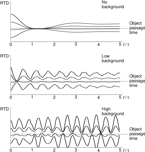
Figure 6: Computer simulations of the adaptation dynamics for the response time differences ${\rm RTD}^{(c,\pm)}(t)$ of 4 classes of neurons ($c=1,2,3,4$). Their receptive fields are arranged in an array of $60\times 60$ retinal locations with 8 neurons per location. The time scale is set by $\tau$, the rise time of corticothalamic postsynaptic potentials; cf. eqn. (5). The stimulus is a coherently moving object (15 dots) without a background (top), with a moderate background (10 dots, middle), and with a strong background (30 dots, bottom). Background dots move at various random speeds, exceeding or less than the object’s speed, in or opposite to the direction of object motion; cf. Fig. 4. Only the 4 trajectories ${\rm RTD}^{(c,+)}(t)$, i.e., representative of the neurons selective for the direction of object motion, are shown. The passage time of object dots is indicated by the straight horizontal line in each graph. The adaptation dynamics converges to a stationary state close to the object’s passage time without a background, and is increasingly oscillatory with increasing background strength. The feedback strength is $\gamma=0.03$ for the no-background case, and $\gamma=0.25$ for the two other cases.

The response time differences ${\rm RTD}^{(c,\pm)}(t)$ of all layer 4 neurons in the system are correlated, both across space and class $c$. The correlation across space is the result of the lateral connectivity of the system; cf. Fig. 5 right. The correlation across classes is mediated by the stimulus; cf. Fig. 6. In particular, neurons of all classes $(c,+)$ are well tuned to an object’s speed at the same time. At such times, therefore, object features elicit strong responses in neurons of all classes $(c,+)$, yielding a high class-averaged response,

$$\langle R^{+}\rangle\,:=\,\frac{1}{n}\sum_{c=1}^{n}R^{(c,+)}\ ;$$ (20)

cf. eqn. (15). At other times the preferences of neurons not only are untuned with respect to the object, but also vary significantly across neurons of different classes $c$. Hence there are no strong class-averaged responses $\langle R^{+}\rangle$, neither to an object, nor to background features.

In turns out that each time course of adaptation is associated with a certain spatiotemporal pattern of cortical activity. For an adaptation time course such as shown at the top of Fig. 6, there are permanent strong class-averaged responses $\langle R^{+}\rangle$ to object features as soon as the RTDs have converged to the object’s passage time. On the other hand, an oscillatory time course as shown at the bottom of the figure is associated with alternating phases of weak and strong responses $\langle R^{+}\rangle$, the strong responses being restricted to object features. In fact, the dynamic RTDs act as a pacemaker for distributed cortical activity. A periodic time structure is imposed that tends to synchronize the firing of layer 4 cells representing the object; see Fig. 7. Oscillations may show up in cortical single cell activity or in multi-unit activity, depending on the nature of the stimulus and the size of RFs. In particular, single neurons show periodic activity, if their responses last longer than one period of oscillation of the RTDs. Their response then comprises several “elementary” response events of the kind marked by a single dot in Fig. 7. The period scales with the rise time $\tau$ of the corticothalamic postsynaptic potentials [see eqn. (5)], and decreases to zero as the stimulus velocity or density becomes very large. Hence, the period can be much shorter than the duration of individual corticothalamic PSPs and even than their rise time $\tau$. The reason is that for a stimulus consisting of features moving at different velocities, PSPs are not initiated in isolation but superimposed upon other PSPs of opposite signs.

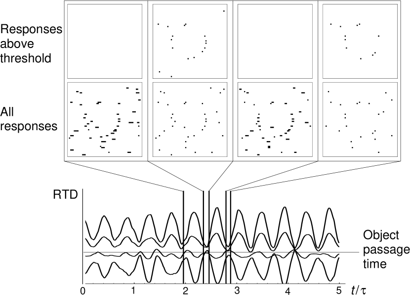
Figure 7: Spatiotemporal pattern of cortical activity in the $60\times 60$ retinotopic array of neurons associated with the adaptation dynamics depicted at the bottom of Fig. 6, re-displayed at the bottom of this figure. The system is stimulated by 15 dots placed on a circle, all moving at a common velocity to the right (object), and 30 dots moving at various random speeds, exceeding or less than the object’s speed, either to the left or to the right; cf. Fig. 4. Whenever the neurons’ preferences, i.e., response time differences (RTDs), get close to the object’s passage time (corresponding to the object’s speed), object dots elicit a strong response in neurons that represent their actual retinal positions. The corresponding array of activity is shown in the panels at the top of the figure. The lower row of panels displays all responses that occur within the indicated intervals of time; the upper row displays only those responses where the class-averaged activity $\langle R^{+}\rangle$ [see eqn. (20)] for a location exceeds a certain threshold. Nearly all supra-threshold activity is related to object features, demonstrating the segmentation of the object against the background. Spurious supra-threshold activity derives from responses to background dots that by chance have speeds very close to the object’s speed. The supra-threshold activity is oscillatory and synchronous. If $\tau$, the rise time of corticothalamic postsynaptic potentials [cf. eqn. (5)], is taken to be 100 ms, the oscillation frequency is roughly 25 Hz in this example.

It is worth noting that a stationary stimulus background and neuronal noise are special cases of directionally unbiased background activity. The system thus also performs segmentation of an object moving across a stationary background and suppression of neuronal noise.

In the present context of stochastic dynamical systems, stability of the dynamics means that at least the first two moments (the mean and the variance) of the RTDs converge to finite values. It can be proved that stability is guaranteed, if $\gamma$, the overall strength of cortical feedback to the LGN [cf. eqn. (13)], is not too large.

To summarize, in this model corticogeniculate loops give rise to object segmentation based on global sampling of velocity features in the visual field. Visual features acquire an enhanced representation in the adaptive motion system by virtue of belonging to a coherent object. The temporal structure of adaptation and, hence, of cortical activity, depends on the statistics of stimulus and noise. With oscillatory dynamics, different objects detected by populations of neurons tuned to different directions of motion turn out to be represented through statistically independent phases of oscillation; cf. Gray et al. (1989). The model can be extended so as to include higher visual areas and in such a way that phases of oscillation become statistically independent for different two-dimensional (2D) directions of motion, i.e., the true directions not accessible to single area 17 cells.

As a consequence of the described dynamics, the control loop for speed preferences recruits neuronal hardware for object representation in a very economic manner in that it avoids at the same time neurons that remain idle and neurons that respond to irrelevant features.

Discussion

Recently it has been proposed that corticogeniculate feedback modulates the spatial layout of simple-cell RFs by exploiting the thalamic burst-tonic transition of relay modes [Wörgötter et al., 1998]. Along a similar line, the main point made by the first part of our modeling is that one should expect a modulatory influence of cortical feedback on the spatiotemporal RF structure of simple cells. More precisely, we observe a shift in the time to the bar-response peak that is opposite for lagged and nonlagged cells; cf. Fig. 2. Assuming (i) an RF layout as usually found for direction-selective simple cells in V1, and (ii) an influence of convergent geniculate lagged and nonlagged inputs on this RF structure, it follows that the observed shifts in response timing affect cortical speed tuning. To the best of our knowledge, nobody has looked for such an effect yet.

Accepting the general conclusion on adaptive cortical speed tuning, the model of the corticogeniculate loop demonstrates what such an effect in the brain may be good for. We have attacked the fundamental sensory task of object segmentation and analyzed a simple implementation of a control loop based on abundant structures of the visual system. The basic idea is to select an important, object-related component of motion. The loop mechanism effectively draws samples of moving features from a retinal region and adapts to the mean of those velocities that are more frequent in one direction than in the opposite, that is, it adapts to an asymmetric peak in the allover velocity density. Such peaks will usually be produced by objects moving over a background; cf. Fig. 4. Features moving at the corresponding velocity acquire an enhanced representation.

The proposed adaptation mechanism could be characterized as pre-attentive, since it requires no “act of will” and no information from higher brain areas where different objects are categorized. Multiple adaptive motion systems could act in parallel for different directions of motion, in different parts of the visual field, and on different spatial scales. From the perspective of efficiency, higher perceptual and attentive mechanisms can be envisaged best to operate on top of a representation level where object-unrelated activity is reduced, as provided by the adaptive motion system. Although at this point it is difficult to pin down the precise mechanisms of contextual effects on neuronal responses in the visual system, it seems clear that modulation related to object segmentation occurs as early as in V1, at least in primates; see Lamme et al. (1998) and references therein.

A critical experimental test of a control loop such as the one analyzed here is to look for changes in spatiotemporal RF structure on a timescale of, say, 100 ms in response to moving, especially large-field, stimuli. It would be interesting to study reverse correlations in the speed or temporal-frequency domain, analogous to work that has uncovered dynamic orientation tuning in the monkey [Ringach et al., 1997].

More detailed modeling is required to compare the oscillations and synchronization that arise in the loop model under certain conditions with recent data on persistent oscillations in area 17 that are preferentially evoked by moving stimuli [Bringuier et al., 1997, Castelo-Branco et al., 1998]. In the loop model, oscillations may arise from visual stimulation at geniculocortical synapses, showing up as periodic excitatory synaptic potentials in cortical neurons. Because of the slow potentials that modulate the GRC states we would expect such oscillations to be at the lower end of the observed frequency spectrum (below, say, 30 Hz); cf. Fig. 7. Clearly, since such periodic inputs are not restricted to layer 4 [Bringuier et al., 1997], intracortical connections have also a role to play, certainly in the propagation of the periodic activity.

As expounded above, the loop model was not designed to fit any particular set of experimental data, and at this stage it does not explain convincingly cortical oscillations. Whatever the details of a control loop, however, a slow modulation of GRC membrane potentials controlled by comparatively fast responses of cortical neurons is likely to produce oscillations under certain conditions. Our argument thus does add a new dimension to the search for the origin of rhythmic and synchronous activity in the low-frequency range.

Great care must be taken when extrapolating from cats to primates. No lagged relay cells have been described in the primate LGN so far. On the other hand, a recent study [Valois & Cottaris, 1998] does suggest a set of geniculate inputs to directionally selective simple cells in macaque striate cortex that is essentially analogous to the lagged-nonlagged set envisaged for cat simple cells. If indeed primates employ a similar system at the lowest level of motion analysis, the corticogeniculate loop would implement at this level the classical Gestalt principle of “common fate”, which recognizes common motion as a powerful cue for object segmentation in humans [Wertheimer, 1958, Julesz, 1971]. Furthermore, we would obtain a new rationale to the nature of the input to neurons in primate area V2 that extract the shape of objects from coherent motion on a background [Peterhans & Baumann, 1994, Peterhans, 1997]. That is to say, V1 detects an object through common motion and V2 then analyzes its shape.

An important side effect of the adaptation mechanism is that it can account for visual stabilization during fixational eye movements. These erratic eye movements cause retinal slips providing motion signals that are directionally unbiased on the timescale of the control loop ($\sim$ 100 ms). Since unbiased motion does not lead to adaptation to any particular velocity, none of the moving features is highlighted. Now, if the brain relies on the activity of adaptively speed-tuned neurons to infer motion in the outside world, no such motion will be inferred from fixational eye movements. Stabilization of the visual world is thus achieved because successive motion signals cancel out in the control loop.

Interestingly, this stabilization mechanism explains the recently reported ‘jitter after-effect’ [Murakami & Cavanagh, 1998]. An observer is first exposed to dynamic random noise for 30 s, and then fixates a larger area of static random noise. The perception is a coherent jitter of the static noise that follows fixational eye movements, specifically, in the region that has not been exposed to the prior random motion. The explanation in terms of the present model relies on the fact that responses of velocity-selective neurons are reduced after stimulation for 30 s [also called ‘adaptation’, but unrelated to the adaptation of speed preferences proposed here; see Hammond et al. (1988)]. As can be seen from eqn. (13), for reduced cortical responses $R_{i}$, $R^{>}_{i}$, $R^{<}_{i}$ to each of the sweeps induced by eye movements, the amplitudes $A_{i}$ of the corticogeniculate potentials [cf. eqn. (6)] become larger. The effect is similar to an increased allover strength $\gamma$ of cortical feedback. So it may be that each brief period of eye-induced motion that normally averages out in adaptation now gives rise to fluctuations of adaptation of sufficient amplitude to evoke enhanced responses outside the region of reduced responsiveness. Thus the same mechanism that ensures stabilization during normal fixation will now signal jitter motion.

The results presented here offer new explanations for data from diverse research. They also suggest new experimental paradigms to test their implications. In case of confirmation, a re-interpretation of a large amount of data on motion processing might be needed.

References

- [Ahmed et al., 1994] Ahmed, B., Anderson, J. A., Douglas, R. J., Martin, K. A. C., & Nelson, J. C. (1994). Polyneuronal innervation of spiny stellate neurons in cat visual cortex. Journal of Comparative Neurology, 341, 39–49.
- [Alonso et al., 1996] Alonso, J. M., Usrey, W. M., & Reid, R. C. (1996). Precisely correlated firing in cells of the lateral geniculate nucleus. Nature, 383, 815–819.
- [Bal et al., 1995] Bal, T., von Krosigk, M., & McCormick, D. A. (1995). Synaptic and membrane mechanisms underlying synchronized oscillations in the ferret LGNd in vitro. Journal of Physiology (Lond), 483, 641–663.
- [Bloomfield & Sherman, 1988] Bloomfield, S. A. & Sherman, S. M. (1988). Postsynaptic potentials recorded in neurons of the cat’s lateral geniculate nucleus following electrical stimulation of the optic chiasm. Journal of Neurophysiology, 60, 1924–1945.
- [Bringuier et al., 1997] Bringuier, V., Fregnac, Y., Baranyi, A., Debanne, D., & Shulz, D. E. (1997). Synaptic origin and stimulus dependency of neuronal oscillatory activity in the primary visual cortex of the cat. Journal of Physiology (Lond), 500, 751–774.
- [Castelo-Branco et al., 1998] Castelo-Branco, M., Neuenschwander, S., & Singer, W. (1998). Synchronization of visual responses between the cortex, lateral geniculate nucleus, and retina in the anesthetized cat. Journal of Neuroscience, 18, 6395–6410.
- [Cleland & Harding, 1983] Cleland, B. G. & Harding, T. H. (1983). Response to the velocity of moving visual stimuli of the brisk classes of ganglion cells in the cat retina. Journal of Physiology (Lond), 345, 47–63.
- [Cleland et al., 1979] Cleland, B. G., Harding, T. H., & Tulunay-Keesey, U. (1979). Visual resolution and receptive field size: Examination of two kinds of cat retinal ganglion cell. Science, 205, 1015–1017.
- [Contreras et al., 1993] Contreras, D., Dossi, R. C., & Steriade, M. (1993). Electrophysiological properties of cat reticular thalamic neurones in vivo. Journal of Physiology (Lond), 470, 273–294.
- [Cox et al., 1998] Cox, C. L., Zhou, Q., & Sherman, S. M. (1998). Glutamate locally activates dendritic outputs of thalamic interneurons. Nature, 394, 478–482.
- [Crick & Koch, 1998] Crick, F. & Koch, C. (1998). Constraints on cortical and thalamic projections: the no-strong-loops hypothesis. Nature, 391, 245–250.
- [Crook et al., 1998] Crook, J. M., Kisvarday, Z. F., & Eysel, U. T. (1998). Evidence for a contribution of lateral inhibition to orientation tuning and direction selectivity in cat visual cortex: reversible inactivation of functionally characterized sites combined with neuroanatomical tracing techniques. European Journal of Neuroscience, 10, 2056–2075.
- [Crunelli & Leresche, 1991] Crunelli, V. & Leresche, N. (1991). A role for gabab receptors in excitation and inhibition of thalamocortical cells. Trends in Neurosciences, 14, 16–21.
- [DeAngelis et al., 1995] DeAngelis, G. C., Ohzawa, I., & Freeman, R. D. (1995). Receptive-field dynamics in the central visual pathways. Trends in Neurosciences, 18, 451–458.
- [Douglas et al., 1995] Douglas, R. J., Koch, C., Mahowald, M., Martin, K. A. C., & Suarez, H. H. (1995). Recurrent excitation in neocortical circuits. Science, 269, 981–985.
- [Ferster et al., 1996] Ferster, D., Chung, S., & Wheat, H. (1996). Orientation selectivity of thalamic input to simple cells of cat visual cortex. Nature, 380, 249–252.
- [Field, 1994] Field, D. J. (1994). What is the goal of sensory coding? Neural Computation, 6, 559–601.
- [Gerstner & van Hemmen, 1992] Gerstner, W. & van Hemmen, J. L. (1992). Associative memory in a network of “spiking” neurons. Network, 3, 139–164.
- [Godwin et al., 1996] Godwin, D. W., Vaughan, J. W., & Sherman, S. M. (1996). Metabotropic glutamate receptors switch visual response mode of lateral geniculate nucleus cells from burst to tonic. Journal of Neurophysiology, 76, 1800–1816.
- [Gray et al., 1989] Gray, C. M., König, P., Engel, A. K., & Singer, W. (1989). Oscillatory responses in cat visual cortex exhibit inter-columnar synchronization which reflects global stimulus properties. Nature, 338, 334–337.
- [Guido et al., 1992] Guido, W., Lu, S.-M., & Sherman, S. M. (1992). Relative contributions of burst and tonic responses to the receptive field properties of lateral geniculate neurons in the cat. Journal of Neurophysiology, 68, 2199–2211.
- [Guido et al., 1995] Guido, W., Lu, S.-M., Vaughan, J. W., Godwin, D. W., & Sherman, S. M. (1995). Receiver operating characteristic (ROC) analysis of neurons in the cat’s lateral geniculate nucleus during tonic and burst response mode. Visual Neuroscience, 12, 723–741.
- [Guido & Weyand, 1995] Guido, W. & Weyand, T. (1995). Burst responses in thalamic relay cells of the awake, behaving cat. Journal of Neurophysiology, 74, 1782–1786.
- [Hammond et al., 1988] Hammond, P., Mouat, G. S., & Smith, A. T. (1988). Neural correlates of motion after-effects in cat striate cortical neurones: monocular adaptation. Experimental Brain Research, 72, 1–20.
- [Hartveit & Heggelund, 1990] Hartveit, E. & Heggelund, P. (1990). Neurotransmitter receptors mediating excitatory input to cells in the cat lateral geniculate nucleus. II. nonlagged cells. Journal of Neurophysiology, 63, 1361–1372.
- [Heggelund & Hartveit, 1990] Heggelund, P. & Hartveit, E. (1990). Neurotransmitter receptors mediating excitatory input to cells in the cat lateral geniculate nucleus. I. lagged cells. Journal of Neurophysiology, 63, 1347–1360.
- [Hirsch et al., 1998] Hirsch, J. A., Alonso, J.-M., Reid, R. C., & Martinez, L. M. (1998). Synaptic integration in striate cortical simple cells. Journal of Neuroscience, 18, 9517–9528.
- [Huguenard & McCormick, 1992] Huguenard, J. R. & McCormick, D. A. (1992). Simulation of the currents involved in rythmic oscillations in thalamic relay neurons. Journal of Neurophysiology, 68, 1373–1383.
- [Humphrey & Weller, 1988a] Humphrey, A. L. & Weller, R. E. (1988a). Functionally distinct groups of X-cells in the lateral geniculate nucleus of the cat. Journal of Comparative Neurology, 268, 429–447.
- [Humphrey & Weller, 1988b] Humphrey, A. L. & Weller, R. E. (1988b). Structural correlates of functionally distinct X-cells in the lateral geniculate nucleus of the cat. Journal of Comparative Neurology, 268, 448–468.
- [Jagadeesh et al., 1993] Jagadeesh, B., Wheat, H. S., & Ferster, D. (1993). Linearity of summation of synaptic potentials underlying direction selectivity in simple cells of the cat visual cortex. Science, 262, 1901–1904.
- [Jagadeesh et al., 1997] Jagadeesh, B., Wheat, H. S., Kontsevich, L. L., Tyler, C. W., & Ferster, D. (1997). Direction selectivity of synaptic potentials in simple cells of the cat visual cortex. Journal of Neurophysiology, 78, 2772–2789.
- [Julesz, 1971] Julesz, B. (1971). Foundations of Cyclopean Perception. Chicago: University of Chicago Press.
- [Katz, 1987] Katz, L. C. (1987). Local circuitry of identified projection neurons in cat visual cortex brain slices. Journal of Neuroscience, 7, 1223–1249.
- [Kistler et al., 1997] Kistler, W. M., Gerstner, W., & van Hemmen, J. L. (1997). Reduction of the hodgkin-huxley equations to a single-variable threshold model. Neural Computation, 9, 1015–1045.
- [Koch, 1987] Koch, C. (1987). The action of the corticofugal pathway on sensory thalamic nuclei: A hypothesis. Neuroscience, 23, 399–406.
- [Kontsevich, 1995] Kontsevich, L. L. (1995). The nature of the inputs to cortical motion detectors. Vision Research, 35, 2785–2793.
- [Kwon et al., 1991] Kwon, Y. H., Esguerra, M., & Sur, M. (1991). NMDA and non-NMDA receptors mediate visual responses of neurons in the cat’s lateral geniculate nucleus. Journal of Neurophysiology, 66, 414–428.
- [Lamme et al., 1998] Lamme, V. A. F., Supèr, H., & Spekreijse, H. (1998). Feedforward, horizontal, and feedback processing in the visual cortex. Current Opinion in Neurobiology, 8, 529–535.
- [Lo & Sherman, 1994] Lo, F. S. & Sherman, S. M. (1994). Feedback inhibition in the cat’s lateral geniculate nucleus. Experimental Brain Research, 100, 365–368.
- [Lu et al., 1992] Lu, S.-M., Guido, W., & Sherman, S. M. (1992). Effects of membrane voltage on receptive field properties of lateral geniculate neurons in the cat: Contributions of the low-treshold ca2+ conductance. Journal of Neurophysiology, 68, 2185–2198.
- [Maex & Orban, 1996] Maex, R. & Orban, G. A. (1996). Model circuit of spiking neurons generating directional selectivity in simple cells. Journal of Neurophysiology, 75, 1515–1545.
- [Mastronarde, 1987a] Mastronarde, D. N. (1987a). Two classes of single-input X-cells in cat lateral geniculate nucleus. I. Receptive-field properties and classification of cells. Journal of Neurophysiology, 57, 357–380.
- [Mastronarde, 1987b] Mastronarde, D. N. (1987b). Two classes of single-input X-cells in cat lateral geniculate nucleus. II. Retinal inputs and the generation of receptive-field properties. Journal of Neurophysiology, 57, 381–413.
- [McClurkin et al., 1994] McClurkin, J. W., Optican, L. M., & Richmond, B. J. (1994). Cortical feedback increases visual information transmitted by monkey parvocellular lateral geniculate nucleus neurons. Visual Neuroscience, 11, 601–617.
- [McCormick & Huguenard, 1992] McCormick, D. A. & Huguenard, J. R. (1992). A model of the electrophysiological properties of thalamocortical relay neurons. Journal of Neurophysiology, 68, 1384–1400.
- [McCormick & von Krosigk, 1992] McCormick, D. A. & von Krosigk, M. (1992). Corticothalamic activation modulates thalamic firing through glutamate “metabotropic” receptors. Proceedings of the National Academy of Sciences USA, 89, 2774–2778.
- [McLean & Palmer, 1989] McLean, J. & Palmer, L. A. (1989). Contribution of linear spatiotemporal receptive field structure to velocity selectivity of simple cells in area 17 of the cat. Vision Research, 29, 675–679.
- [Mukherjee & Kaplan, 1995] Mukherjee, P. & Kaplan, E. (1995). Dynamics of neurons in the cat lateral geniculate nucleus: In vivo electrophysiology and computational modeling. Journal of Neurophysiology, 74, 1222–1243.
- [Murakami & Cavanagh, 1998] Murakami, I. & Cavanagh, P. (1998). A jitter after-effect reveals motion-based stabilization of vision. Nature, 395, 798–801.
- [Murthy et al., 1998] Murthy, A., Humphrey, A. L., Saul, A. B., & Feidler, J. C. (1998). Laminar differences in the spatiotemporal structure of simple cell receptive fields in cat area 17. Visual Neuroscience, 15, 239–256.
- [Orban et al., 1981] Orban, G. A., Kennedy, H., & Maes, H. (1981). Response to movement of neurons in areas 17 and 18 of the cat: Velocity sensitivity. Journal of Neurophysiology, 45, 1043–1058.
- [Pape et al., 1994] Pape, H. C., Budde, T., Mager, R., & Kisvarday, Z. F. (1994). Prevention of Ca(2+)-mediated action potentials in GABAergic local circuit neurones of rat thalamus by a transient K+ current. Journal of Physiology (Lond), 478, 403–422.
- [Peterhans, 1997] Peterhans, E. (1997). Functional organization of area V2 in the awake monkey. In J. H. Kaas, K. Rockland, & A. Peters (Eds.), Cerebral Cortex, volume 12 (pp. 335–357). New York: Plenum Press.
- [Peterhans & Baumann, 1994] Peterhans, E. & Baumann, R. (1994). Elements of form processing from motion in monkey prestriate cortex. Society of Neuroscience Abstract, 20, 1053.
- [Reid & Alonso, 1995] Reid, R. C. & Alonso, J. M. (1995). Specificity of monosynaptic connections from thalamus to visual cortex. Nature, 378, 281–284.
- [Reid et al., 1991] Reid, R. C., Soodak, R. E., & Shapley, R. M. (1991). Directional selectivity and spatiotemporal structure of receptive fields of simple cells in cat striate cortex. Journal of Neurophysiology, 66, 505–529.
- [Reinagel et al., 1999] Reinagel, P., Godwin, D., Sherman, S. M., & Koch, C. (1999). Encoding of visual information by lgn bursts. Journal of Neurophysiology, 81, 2558–2569.
- [Ringach et al., 1997] Ringach, D. L., Hawken, M. J., & Shapley, R. (1997). Dynamics of orientation tuning in macaque primary visual-cortex. Nature, 387, 281–284.
- [Saul & Humphrey, 1990] Saul, A. B. & Humphrey, A. L. (1990). Spatial and temporal response properties of lagged and nonlagged cells in the cat lateral genicualte nucleus. Journal of Neurophysiology, 64, 206–224.
- [Saul & Humphrey, 1992a] Saul, A. B. & Humphrey, A. L. (1992a). Evidence of input from lagged cells in the lateral geniculate nucleus to simple cells in cortical area 17 of the cat. Journal of Neurophysiology, 68, 1190–1207.
- [Saul & Humphrey, 1992b] Saul, A. B. & Humphrey, A. L. (1992b). Temporal-frequency tuning of direction selectivity in cat visual cortex. Visual Neuroscience, 8, 365–372.
- [Sherman & Guillery, 1996] Sherman, S. M. & Guillery, R. W. (1996). Functional organization of thalamocortical relays. Journal of Neurophysiology, 76, 1367–1395.
- [Sherman & Koch, 1986] Sherman, S. M. & Koch, C. (1986). The control of retinogeniculate transmission in the mammalian lateral geniculate nucleus. Experimental Brain Research, 63, 1–20.
- [Sillito et al., 1994] Sillito, A. M., Jones, H. E., Gerstein, G. L., & West, D. C. (1994). Feature-linked synchronization of thalamic relay cell firing induced by feedback from the visual cortex. Nature, 369, 479–482.
- [Singer, 1994] Singer, W. (1994). A new job for the thalamus. Nature, 369, 444–445.
- [Suarez et al., 1995] Suarez, H., Koch, C., & Douglas, R. (1995). Modeling direction selectivity of simple cells in striate visual cortex within the framework of the canonical microcircuit. Journal of Neuroscience, 15, 6700–6719.
- [Tsumoto et al., 1978] Tsumoto, T., Creutzfeldt, O. D., & Legendy, C. R. (1978). Functional organization of the corticofugal system from visual cortex to lateral geniculate nucleus in the cat (with an appendix on geniculo-cortical mono-synaptic connections). Experimental Brain Research, 32, 345–364.
- [Tsumoto & Suda, 1980] Tsumoto, T. & Suda, K. (1980). Three groups of cortico-geniculate neurons and their distribution in binocular and monocular segments of cat striate cortex. Journal of Comparative Neurology, 193, 223–236.
- [Valois & Cottaris, 1998] Valois, R. L. D. & Cottaris, N. P. (1998). Inputs to directionally selective simple cells in macaque striate cortex. Proceedings of the National Academy of Sciences USA, 95, 14488–14493.
- [von Krosigk et al., 1999] von Krosigk, M., Monckton, J. E., Reiner, P. B., & Mccormick, D. A. (1999). Dynamic properties of corticothalamic excitatory postsynaptic potentials and thalamic reticular inhibitory postsynaptic potentials in thalamocortical neurons of the guinea-pig dorsal lateral geniculate nucleus. Neuroscience, 91, 7–20.
- [Wertheimer, 1958] Wertheimer, M. (1958). Principles of perceptual organization. In D. C. Beardslee & M. Wertheimer (Eds.), Readings in Perception (pp. 115–135). Princeton, NJ: van Nostrand.
- [Wörgötter et al., 1998] Wörgötter, F., Suder, K., Zhao, Y., Kerscher, N., Eysel, U. T., & Funke, K. (1998). State-dependent receptive-field restructuring in the visual cortex. Nature, 396, 165–168.