A simulation study of the dynamics of a driven filament in an Aristotelian fluid

Abstract

We describe a method, based on techniques used in molecular dynamics, for simulating the inertialess dynamics of an elastic filament immersed in a fluid. The model is used to study the ”one-armed swimmer”. That is, a flexible appendage externally perturbed at one extremity. For small amplitude motion our simulations confirm theoretical predictions that, for a filament of given length and stiffness, there is a driving frequency that is optimal for both speed and efficiency. However, we find that to calculate absolute values of the swimming speed we need to slightly modify existing theoretical approaches. For the more realistic case of large amplitude motion we find that while the basic picture remains the same, the dependence of the swimming speed on both frequency and amplitude is substantially modified. For realistic amplitudes we show that the one armed swimmer is comparatively neither inefficient nor slow. This begs the question, why are there little or no one armed swimmers in nature?

PACS

1 Introduction

For a class of biologically important polymeric materials elasticity is crucial. Their typical lengths (microns or less) are comparable with the scale on which rigidity prevents them from collapsing. The cytoskeletal filaments actin and microtubules [1] fall in this category, as do cilia and flagella. The latter are motile assemblies of microtubules and other proteins. Because of their size and typical velocities, the motion of these filaments is nearly always in the low Reynolds number regime. This is an inertialess, Aristotelian, world where the dynamics of a surrounding fluid become time-reversible. As a notable consequence, it is difficult to generate any propulsion on this scale [4]. Nonetheless, cytoskeletal filaments are involved in cellular and microorganism motility. Perhaps the most widely known example is that of the flagellum of a sperm cell, that enables it to swim along the ovaric tubes. The internal drive of a flagellum, however, is rather complicated [2]. It involves many internal degrees of freedom and active components. On the other hand, modern micromanipulation techniques, such as optical and magnetic trapping, open up the possibility of perturbing otherwise passive filaments with a simplified and controlled drive. This provides a potentially useful model system for which one may study the fundamentals of motility.

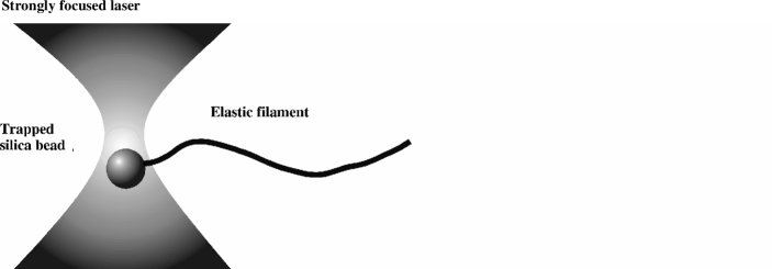
Figure 1: Schematic of a micromanipulation experiment that allows one to apply a controlled drive to a inert filament.

It is this problem we concern ourselves with here. Specifically, we consider the flexible one-armed swimmer. That is, an elastic filament that is wiggled at one end. If the filament were rigid, the reversible motion of the surrounding fluid would ensure that this mechanism generates no propulsion (the “scallop theorem” as Purcell termed it). However, the flexibility of the arm breaks the time reversal symmetry for the motion of the assemblage. This makes propulsion, in principle, possible. For any microscopic filament the factors that determine its dynamic behavior are the same. Namely, the equations of motion will be essentially inertialess. The motion itself will be determined by a balance between forces driving the filament, friction forces exerted as the surrounding fluid opposes any motion, and bending forces that try to restore the (straight) equilibrium state. For relatively simple model systems, there has recently been theoretical progress in solving analytically the “hyperdiffusion” equation that, in the limit of small amplitude motion, describes the movement of such a filament. Wiggins and Goldstein [6] considered the motion of a single filament driven at one end by an external perturbation. Their analysis emphasized that there are two very different regimes; one where bending forces dominate and the filament behaves like a rigid rod, and a second where the viscous damping of the fluid has the effect of suppressing the propagation of elastic waves. For the one armed swimmer, this leads to an optimal set of parameters that maximize either the swimming speed or swimming efficiency. The same analysis gives predictions for the shape of such a wiggled filament that can be compared with the response observed in a micro-manipulation experiment [5]. By comparing experimental results with theory, structural properties of the filament were inferred.

Wiggins and Goldstein consider the flexible one armed swimmer in the limit of small amplitude motion. With the assumption of inertialess dynamics, one can derive the following equation [6] [8] [10] for the function $h(s,t)$, describing the displacement of the filament from the horizontal axis as a function of time $t$ and arclength $s$.

$$\xi_{\perp}\partial_{t}h=-k\Delta^{2}h$$ (1)

Here $\xi_{\perp}$ determines the viscous force, treated as simply a transverse viscous drag and $k$ the stiffness of the filament. This “hyperdiffusion” equation has to be solved subject to appropriate boundary conditions (corresponding to different forms of external driving). Simple active driving mechanisms could be an oscillating constraint on the end position, or an oscillatory torque applied at one extremity. The former can be regarded as the simplest example of what has been called elastohydrodynamics as it involves the balance of viscous and elastic forces. The latter is a more plausible biological mechanism as it involves no net external force. Both these mechanisms are considered by Wiggins and Goldstein and we also consider both here.

To summarize the predictions of the theory, for a given amplitude of driving the remaining parameters can be grouped together to define a dimensionless “Sperm number”,

$$Sp={\left(\frac{l^{4}\omega\xi^{\perp}}{k}\right)}^{\frac{1}{4}}$$ (2)

where $l$ is the length of the filament and $\omega$ the wiggling frequency.

This characterizes the relative magnitudes of the viscous and bending forces. A low value implies that bending forces dominate, a high value viscous forces. As a function of the Sperm number, the theory predicts

• The swimming speed and efficiency (defined as the amount of energy consumed, relative to the amount of energy required to simply drag a passive filament through the fluid at the same velocity), go to zero as Sp goes to zero. This is the stiff limit where the motion is reversible and the scallop theorem applies

• At a sperm number Sp$\simeq 4$ there is a maximum in the both the swimming speed and efficiency (although not at exactly the same value)

• At high sperm numbers a plateau region where the speed and efficiency become independent of Sp, albeit at values lower than the peak.

In this paper we describe a numerical model that allows us to simulate such a driven filament. With the model we can calculate the dynamics, free from restrictions such as small amplitude motion, and with greater scope to specify the type of active forces driving the motion and the boundary conditions applicable for a given physical situation. With such a model, we can test theoretical predictions and also study more complex problems where no analytic solution is available. Here we do both. Looking at small amplitude motion we compare with the theory. Moving on to large amplitude motion we establish to what extent the small amplitude approximation limits the theory.

2 Model and Simulation

Our model solves the equations of motion of a discretized elastic filament immersed in a low Reynolds number fluid. Any form of internal and external forcing can be imposed but we restrict ourselves here to an active force, acting on one extremity, that is periodic in time. The hydrodynamics is kept to the approximation of slender body flow [3], where the local velocity-force relation is reduced to a simple expression in terms of friction coefficients that are shape and position independent. They do nonetheless reflect the difference between friction transverse and longitudinal to the filament. For the problems we are concerned with here the planar driving forces produce planar motions. The model would apply equally well were this not to be the case.

Considering a continuous description of the filament in space and time, one can specify this at any given instant $t$ by a curve $\mathbf{r}(s,t)$, giving a point in space for any value of the arclength parameter $s$ (figure 2).

Figure 2: Curve describing the shape of the filament. $\mathbf{n}(s,t)$ and $\mathbf{t}(s,t)$ are the local normal and tangent unit vector respectively. $\psi(s,t)$ is the angle formed with the x axis.

To describe the dynamics we need the local forces acting on the filament. The latter are related to the energy of the model system. Specifically, we have

• A bending elasticity, described by the Hamiltonian

  $$H=\frac{1}{2}k\int_{0}^{L}C(s)^{2}ds$$ (3)

  where $C(s)=\left(\frac{\partial^{2}\mathbf{r}}{\partial s^{2}}\right)^{2}$ is the local curvature and $k$ the stiffness.

• A constraint of inextensibility, which can be expressed in terms of the tangent vector as

  $$\left|\frac{\partial\mathbf{r}}{\partial s}\right|=1$$

  and imposes the condition that the filament is, to a first approximation, inextensible.

• An over-damped (negligible mass) equation of motion, which can be written as

  $$\partial_{t}\mathbf{r}(s,t)=-\left(\frac{1}{\xi_{\parallel}}\hat{\mathbf{t}}\hat{\mathbf{t}}+\frac{1}{\xi_{\perp}}\hat{\mathbf{n}}\hat{\mathbf{n}}\right)\frac{\delta H}{\delta\mathbf{r}(s)}$$ (4)

  Here, following slender-body theory, the effect of the surrounding fluid is taken as a drag force that is proportional and opposite to the local velocity. This is anisotropic due to the elongated shape of the filament. This requires the presence of a longitudinal drag coefficient $\xi_{\parallel}$ associated with the projector $\hat{\mathbf{t}}\hat{\mathbf{t}}$ along the tangent vector $\mathbf{t}$, together with a transverse coefficient $\xi_{\perp}$ acting along the normal vector $\mathbf{n}$.

Accordingly, one obtains two equations of motion, one for the evolution of the filament shape, and the other for the tension force $\tau(s,t)$, that enforces locally the inextensibility constraint. Expressing the curve shape as the angle $\psi(s,t)$ that its local tangent forms with a fixed $\hat{\mathbf{x}}$ direction, one can write these equations as (see [8]):

$$\partial_{t}\psi=\frac{1}{\xi_{\perp}}\left(-k\partial_{s}^{4}\psi+\tau\partial_{s}^{2}\psi+\partial_{s}\psi\partial_{s}\tau\right)+\frac{1}{\xi_{\parallel}}\partial_{s}\psi\left(k\partial_{s}^{2}\psi\partial_{s}\psi+\partial_{s}\tau\right)$$ (5)

and

$$\partial_{s}^{2}\tau-\frac{\xi_{\parallel}}{\xi_{\perp}}(\partial_{s}\psi)^{2}\tau=-k\partial_{s}(\partial_{s}\psi\partial_{s}^{2}\psi)+\frac{\xi_{\parallel}}{\xi_{\perp}}\partial_{s}\psi(-k\partial_{s}^{3}\psi)$$ (6)

The two nonlinear equations above have then to be solved subject to appropriate boundary conditions. For example, no external forces and torques for a free tail. For the wiggling problems we examine here, the non-equilibrium drive (oscillating end position or torque) is, in these terms, simply a time-dependent boundary condition. Through a functional expansion about the obvious solution for zero drive $\psi_{0}(s,t)=0$, $\tau_{0}(s,t)=0$,

$$\begin{array}[h]{cc}\psi&=\epsilon\psi_{1}+\epsilon^{2}\psi_{2}+...\\ \tau&=\epsilon\tau_{1}+\epsilon^{2}\tau_{2}+...\end{array}$$ (7)

it is straightforward to obtain, to second order in $\epsilon$ the (decoupled) equations

$$\partial_{t}\psi_{1}=-\frac{k}{\xi_{\perp}}\partial_{s}^{4}\psi_{1}$$

for $\psi_{1}$ and

$$\partial_{t}^{2}\tau_{2}=-\partial_{s}(k\partial_{s}\psi_{1}\partial_{s}^{2}\psi_{1})-\frac{\xi_{\parallel}}{\xi_{\perp}}(k\partial_{s}\psi_{1}\partial_{s}^{3}\psi_{1})$$

for the tension. Furthermore, expressing the shape of the filament in terms of the transverse and longitudinal “absolute” displacements $u(s,t)$ and $h(s,t)$ from the direction $\hat{\mathbf{x}}$ of the filament’s resting position, one gets to equation 1 for the time evolution of $h$ to second order in $\epsilon$.

In the simulations we use a particle model to solve equations 5 and 6 numerically using an approach similar to molecular dynamics. Time is discretized and the filament is described as a set of $n$ point particles rigidly connected by $n-1$ “links”. The interaction between the particles is constructed so as to reproduce the appropriate collective behavior. For convenience in implementing the algorithm, we do not simulate the over-damped motion, given by equation 4 directly. This would correspond to the zero mass case. Rather, we solve the damped Newton equation for an object with “small” total mass $m$. By making the mass small enough we can reproduce the required inertia-less mass independent behavior [14].

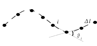
Figure 3: Discretization of the filament

The bending forces acting on the individual particles are defined as follows. If we consider three consecutive discretization points, their positions will lie on one unique circle of radius, $R_{i}$,

$$C_{i}^{2}={\left(\frac{1}{R_{i}}\right)}^{2}=\frac{2}{{\Delta l}^{2}}\left(1-\cos(\theta_{i})\right)$$

where $\Delta l=L/(n-1)$ is the link length and $\theta_{i}$ the angle between two links at the position of bead $i$. We introduce a bending potential $U_{i}$ of the form

$$U_{i}=A\left(1-\cos(\theta_{i})\right)$$

so that the total bending energy will be

$$H=\sum_{i=2}^{n}U_{i}=A\sum_{i=2}^{n}\left(1-\cos(\theta_{i})\right)$$

which we can compare with a discretization of the integral in 3

$$H=\frac{k}{2}\Delta l\sum_{i=2}^{n}{\left(C_{i}^{2}\right)}$$

This leads to the identification $A=\frac{k}{\Delta l}$. A more sophisticated approach [11], where the problem is mapped onto the worm-like chain model of Kratky and Porod [12], leads to a slightly different expression, $A=\frac{n-1/2}{L}k$. The two expressions are equivalent in the limit $n\rightarrow\infty$, where they reproduce the bending energy of the continuous filament, but they differ for the finite number of beads used in the model. The latter leads to faster convergence in the results as the number of discretization point particles is increased. We therefore chose to adopt it.

The inextensibility constraint is implemented by introducing equal and opposite forces along the links between particles. The magnitude of the forces is computed by imposing a fixed distance $\Delta l$ between consecutive beads at each time step. This is a straightforward matter from the computational point of view, as it involves only the inversion of a tridiagonal matrix [15].

The viscous drag forces acting on the particles of the model filament are taken as $F_{ij}=-\delta_{ij}(\xi_{\parallel}\hat{\bf t}\hat{\bf t}+\xi_{\perp}\hat{\bf n}\hat{\bf n})\mathbf{v}$, where $\hat{\bf t}$ and $\hat{\bf n}$ are respectively unit vectors parallel and normal to the filament, $\xi_{\parallel},\xi_{\perp}$ are the longitudinal and transverse friction coefficients, and $\mathbf{v}$ is the local velocity. This means that hydrodynamics is approximated as a local effect on the filament so the hydrodynamic interaction between different points along the curve does not vary. The global shape of the curve enters only through the anisotropy of the viscous drag coefficients acting on individual points. The ratio of the two coefficients depends on the geometric details of the filament analyzed. For cilia, flagella, or cytoskeletal filaments, its value is typically taken between $1.4$ and $2$ [9]. We chose to adopt an arbitrary $1.5$ in most of our simulations, but we also explored different values, including the cases where the two drags are equal or their ratio is lower than one. The time evolution is evaluated in a molecular dynamics-like fashion, with the only slight subtlety that the Verlet algorithm has to be modified to allow for the velocity dependent anisotropic viscous force [14]. Finally, the active drive at the head is simply implemented as a constraint on the first or first two particles. That is, $y_{1}=h_{0}\cos(\omega t)$ for the oscillating constraint or a periodic torque, $T_{x}=B\sin\left(\omega t\right)$ realized as a couple of forces applied to the first two beads. Here $\omega$ is the driving frequency.

3 Results for small deviations

3.1 Wave Patterns

Using the ”Sperm Number” Sp defined in section 1, we can characterize the relative magnitude of the viscous and bending forces. To recapitulate, a low value of Sp indicates that bending forces dominate, whereas for low values the dominant forces are viscous. One reason for defining this number comes from the solution of equation 1 [6] [14]. In fact, Sp can be interpreted as a rescaled filament length, where the rescaling factor is a characteristic length $l_{*}=\left(\frac{k}{\omega\xi_{\perp}}\right)^{1/4}$ that can be used to non-dimensionalize the equation. Both for the oscillating constraint and oscillating torque we recover the fact that the dynamic response, for a fixed driving amplitude, is solely dependent on Sp.

In figure 4 we have plotted the wave patterns for the filament at different values of Sp. These results were obtained using the oscillating constraint. That is, the transverse position at the wiggled end is forced to be sinusoidal in time. The amplitude of the motion is small, the maximum displacement being $1\%$ of the filament length. The pictures can be interpreted as “stroboscopic snapshots” of the filament’s motion. For small Sp, bending forces dominate and the stiff filament pivots around a fixed point. This motion is virtually symmetric with respect to time inversions (“reciprocal”). As Sp increases a (damped) wave travels along the filament and time reciprocity is broken. For increasing values of Sp, viscous forces overcome elastic forces and the characteristic length scale of damping of the traveling wave becomes smaller. This requires that the spacing between the beads in our discrete model must also be reduced to give a fixed degree of accuracy. The number of beads in the model (or equivalently the inverse bead spacing) were thus increased with increasing Sp to ensure that the results are within a percent of the true, continuum, values. The oscillating torque gives qualitatively similar results.

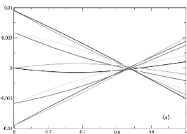
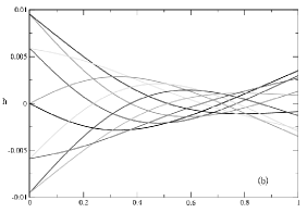
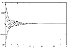
Figure 4: Waveforms of the filament oscillations for different values of Sp. (a) Low Sperm number (Sp$=2.46$). The motion consists of pivoting oscillations about a fixed point. (b) Intermediate Sperm number (Sp$=4.29$). A damped wave propagates along the filament making the movement non-reciprocal in time. (c) High Sperm Number (Sp$=22.61$). The propagating wave is damped within a length that becomes smaller with increasing Sp.

All these results are in agreement with the analytical findings of Wiggins and Goldstein [6] in the small amplitude approximation. The agreement is also quantitative.

3.2 Swimming

From the simulation we are also able to compute the velocity and efficiency of the movement generated transverse to the wiggling direction (due to the propulsive force generated by the presence of the active force) as a function of Sp. We define swimming of the immersed object as the generation of motion, through modifications of shape, in the direction along which no external force acts. Both the speed and efficiency, as Wiggins and Goldstein predict, display an optimum value at intermediate (but different) values of Sp. Subsequently they reach a plateau as viscous forces begin to dominate (Sp increases).

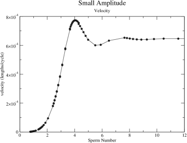
Figure 5: Propulsive velocity as a function of Sperm number for small amplitude oscillation ($h_{0}=0.01l$) of the constraint at the ”head” end of the filament. The function goes as the fourth power of Sp for small values of this number, reaches an optimum, then relaxes to a plateau.

According to the “scallop theorem” of low Reynolds number hydrodynamics, reciprocal (time reversion invariant) motion generates no swimming [4]. This is a consequence of the time-reversibility of Stokes flow and sets an important condition for the ability of microorganisms to swim. In our case, this implies that we expect no swimming as Sp approaches zero and the motion approaches reciprocity. This is confirmed by the result in figure 5. The optimum of the velocity is thus the result of a trade-off between non-reciprocity of the motion and damping of the traveling wave.

At this point we should also be able to compare our results quantitatively with those obtained analytically using the approximation of small deviations. However, in this respect the theoretical analysis is somewhat misleading. Computing the time average of the force, as in [5] and [6], yields the expression

$$\bar{F}=\frac{h_{0}^{2}\xi_{\perp}\omega}{4\sqrt{2}}\textrm{Y(Sp)}$$

where Y(Sp) is a scaling function that can be computed exactly (figure 6). This expression depends only on the transverse friction coefficient and does not reduce to zero when $\xi_{\perp}=\xi_{\parallel}$. As such, it is impossible to relate this to the swimming speed. This follows from the fact that if the condition $\xi_{\perp}=\xi_{\parallel}$ is satisfied there can be no swimming. It is easy to show this must be the case (basically as a consequence of Newton’s third law). The main reason is that, if one considers one particle (i.e. a short piece of filament), the effective viscous drag that it experiences at any moment in time is decoupled from the local configuration of the filament if there is no anisotropy in the friction coefficients. Averaged over one cycle, this always leads, effectively, to reciprocal motion. All the forces sum to zero so there can be no displacement. This is shown more formally in the Appendix. Furthermore, our simulations do indeed yield no average velocity if the two friction coefficients are equal (we use this to check that there is no “numerical” swimming, due to the accumulated errors in the simulation). Thus the result given in equation 3.2, whilst analytically exact, is misleading (probably due to subtleties in the formalism of the over-damped equation of motion). To correct for this anomaly we used the theory and computed instead, following the procedure outlined in [8], the time average of the swimming velocity given the analytical solution for the shape [5]. This yields (see Appendix)

$$v=h_{0}^{2}\left(1-\frac{\xi_{\perp}}{\xi_{\parallel}}\right)\frac{\omega}{4\sqrt{2}L}\textrm{Y(Sp)}$$ (8)

where Y(Sp) is again the scaling function specified by Wiggins and Goldstein in computing the average force (figure 6). Note that this expression (equation 8) predicts no swimming when

• Sp $=0$ and the motion is reciprocal in time (see fig. 2)

• When the two drag coefficients $\xi_{\perp}$ and $\xi_{\parallel}$ are equal.

consistent with both the scallop theorem and Newton’s third Law.

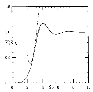
Figure 6: The function Y(Sp) from Wiggins et al..

It also predicts a change in the swimming direction if the friction coefficients are interchanged. Curiously, this reversal of direction has a biological analogue in the organism Ochromonas which has a flagellum decorated by lateral projections (mastigonemes) and swims in the same direction as that of the propagating wave. The body follows the flagellum, instead of preceding it as in sperm cells ( [1], p.11).

Comparing the modified analytical expression for the swimming speed with the simulations, the essential features predicted are obviously present. Both approach zero as $\textrm{Sp}^{4}$ for small Sperm numbers, but with increasing Sperm number display a maximum. In fact, a careful analysis shows that the agreement, in the small amplitude limit, is exact. The presence of a plateau at high Sp is hard to interpret, in the sense that it predicts velocities for even the “infinitely floppy” filament, where the wave pattern is completely damped in an infinitely small region close to the driven extremity. However, in our simulations we see the velocity dropping only when the size of this damping region is comparable to the distance between two subsequent discretization points, so we have to confirm the analytical result and explain this oddity, as we will see, as a feature of the small deviation approximation.

4 Large Angular Deviations

Our simulation contains the full nonlinear model for the dynamics of the filament, its only limitation being the discretization of space and time. Therefore, it is interesting to use it to investigate the limitations of the analytical model when the motion involves shapes that deviate significantly from straight. This is also closer to a real experimental (or biological) situation. The shapes we found often cannot be described by a function, as the displacement from the horizontal axis is not single-valued. This can be observed in figure 7, where we show an example of wave pattern for the case of oscillating large amplitude constraint. In this case, the maximum transverse displacement is $60\%$ of the tail length. Looking at this figure, it is obvious that the behavior predicted by equation 1 will be substantially modified.

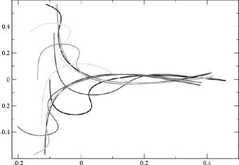
Figure 7: Wave patterns for the case of an oscillating constraint with amplitude $h_{0}=0.6\ l$ at $\textrm{Sp}=2.8$.

The first notable area of disagreement is at high values of the Sperm number ($\textrm{Sp}>>1$) where we no longer find a plateau but a slow and steady drop in both speed and efficiency (figure 8). This effect is clearly a consequence of the non-negligible amplitude of the motion because for smaller amplitudes a plateau is indeed reached. This is a limitation of the theory, one respect in which large amplitude motions differ from the small amplitude limit. Further the results for a dimensionless amplitude of $0.25$ display a transient plateau that subsequently decays to zero. This implies that for any finite amplitude the dimensionless swimming speed always goes zero for large enough Sp. The smaller the amplitude the longer the plataeu persists, but only for negligible amplitude, is it the asymptotic behaviour. It should be noted that figures 5 and 8 should be interpreted with care. The swimming velocity is plotted in units of the fraction of the length per cylce. To obtain absolute swimming speeds, for a tail of given length and stiffness, we would need to multiply this dimensioless swimming speed by the frequency. The frequency itself is proportional to Sp⁴ so a plateau in these plots still implies a swimming speed increasing proportionally with $\omega$. The drop from the plateau means that the actual swimming speed will increase with frequency, but a a slower rate. Thus, in practice the one armed swimmer can go as fast as he or she likes by wiggling fast enough.

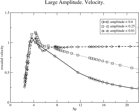
Figure 8: Velocity versus sperm number for different values of the amplitude $h_{o}$ in the case of oscillating constraint. The velocities have been rescaled to show the drop of the plateau.

Secondly, we find that the dependence of the optimum swimming speed, equation 8 predicts as the square of the amplitude of the oscillating constraint, becomes linear for higher amplitude oscillations (figure 9).

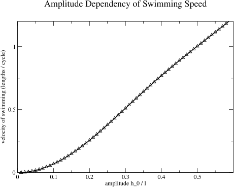
Figure 9: Velocity versus amplitude for the case of an oscillating constraint close to the optimum for the speed (Sp = 4).

Thus far, we have not been able to show why this is the case, but we believe it is related to the following. For small amplitude motion the elastic wave simply propagates along an essentially straight filament. As the amplitude increases, this is no longer true because the filament itself is significantly bent and, so far as the damping is concerned, it is the distance along the filament that is relevant. This is no longer the same quantity as the absolute distance. This seems to lead to an increase in the effective length of the filament.

From these results it is clear that the amplitude of the drive for which the small deviation approximation breaks down depends on the value of Sp, being greater for smaller Sperm Numbers. At the optimal value for the speed, Sp$=4$, the approximation holds for maximum transverse displacements of up to $20\%$ of the tail length, which is well beyond the point one would expect the assumptions to be valid. However, for a realistic experiment with actin or a microtubule, the values of Sp are much higher than $4$, and the value for the theshold is much lower. For example, for an actin filament of $50\mu m$, driven at 1 cycle/second at an amplitude of $25\%$ of its length, we estimated a speed of about $1,7\mu m/sec$ with the small deviation model, whereas our simulation predicts a reduction of this value by a factor $1/4$.

For external driving in the form of a torque applied at one end, we have only considered large amplitude motion. Specifically, the pre-factor $B$ was adjusted to produce a maximum angle at the driven end of $60^{o}$. This clearly violates the small angle approximation of Wiggins and Goldstein [6] but is more consistent with the head deflections found in practice for swimming organisms. In figure 10 we plot the efficiency and the mean velocity as functions of Sp. Once again, the two curves agree qualitatively with those found analytically by Wiggins and Goldstein in that there is a peak speed and efficiency. The values are at slightly different values of Sp and, because the small angle approximation is violated, not quantitatively predicted by equation 8.

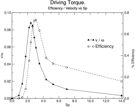
Figure 10: Velocity / efficiency versus Sp for the case of driving torque.

We should add here a few comments. Notably, the peak efficiency of less than $1\%$ seems very low. However, this depends strongly on the amplitude of the motion. If we go above the $60^{o}$ limit we have imposed here for the torque, or to driving amplitudes of greater than half the length of the filament, it is possible to reach values of $2\%$ before the motion becomes unstable. This is similar to the efficiency typical for both the helical screw mechanism used by bacteria and the sperm motion [14]. Thus, the one-armed swimmer operating at peak efficiency is a plausible and not especially inefficient entity. Note also that the efficiency (which is dimensionless), as well as the swimming speed, decays to zero rather than reaching a plateau value. This means that in absolute terms the one-armed swimmer can carry on with increasing speed by increasing its wiggling frequency but only at the price of decreasing efficiency.

5 Conclusions

We have described a simulation method that can be used to study the motion of driven elastic filaments in a low Reynolds number flow. Here, the hydrodynamic friction is treated quite simply, consistent with comparing with analytically tractable theories. A more complete calculation of the hydrodynamic effects would no doubt be instructive. In particular, the friction coefficients are not, as we assume here, independent of distance along the filament. At the expense of a little more computational complexity, such effects could be incorporated into our model in a straightforward manner. We showed that, within this approximation, the picture suggested by Wiggins and Goldstein for the linear regime of small angular deviations from the straight position is essentially correct. Our results for the motion of the filament, show good agreement with their analytical calculations. There is an optimal balance between bending forces and viscous forces that leads to a maximum propulsive speed and efficiency. However, in one quantitative respect our results suggest that their analysis is limited. We could not relate their expression for the average force exerted by the filament to the swimming speed. Instead, we used their model to compute an expression for the average swimming velocity that is physically more plausible and agrees with the simulation results.

For large amplitude motion, we found that the dependence of the swimming speed on both sperm number and amplitude was significantly modified relative to the small amplitude case. Further, we postulate that this is due to the fact that in a highly distorted filament the wave travels along a notably different path than is the case for small amplitude motion. A quantitative understanding of this effect is still, however, lacking. Nonetheless, the general picture derived from the linear theory, of an optimal compromise between the bending required to break time reversibility and excessive damping suppressing motion along the filament, remains valid. The most significant difference we found was that there will come a point beyond which increasing the wiggling frequency leads to a drop in efficiency. The theory, on the other hand, predicts that the efficiency remains constant.

For realistic amplitudes of oscillation, we found that one-armed swimming is, speed and efficiency-wise, a plausible strategy a microorganism might use to get around. It is also a sight simpler than the helical screw mechanism used by most bacteria. This requires a rotary joint [1]. Nonetheless, while we stand open to correction, we have not been able to identify a single organism that actually adopts this strategy. Perhaps the most interesting question surrounding the one armed swimmer is thus: why doesn’t it exist? Based on our results, we suggest two hypotheses. First, localized bending of the tail requires implausibly high energy densities. Second, the existence of an evolutionary barrier. It is useless trying to swim with a short or slow moving tail. Note that at small Sp (that is, low frequency and or a short appendage) there is nothing to be gained in terms of motility. This is not the case for either the helical screw mechanism, commonly used by bacteria, or the traveling wave, used by spermatozoa. Both of these give a maximum swimming speed and efficiency at low sperm numbers.

Regarding experimental studies of in vitro motility, one main problem so far is that the force involved has been too small to be detectable with an optical trapping experiment. This limitation could be resolved simply by time, as it is reasonable to expect that the resolution of experiments will improve. On the other hand, by means of the model one could try to find the region of the parameter space where this force is expected to be highest, and try to design an “optimal experiment” where the motility could actually be quantified.

We would like to thank Catalin Tanase, Marileen Dogterom and Daan Frenkel for discussion and help.

Appendix

5.1 Unequal friction coefficients as a condition for motility

It is possible to show that there can be no movement if the viscous drag coefficients are equal. Most conveniently, we work with the the discrete model. Since the discrete model produces the continuum result in the limit that the number of beads $N$ goes to infinity, there is no loss of generality (so long as the answer does not depend on $N$). The equation of motion for the center of mass is

$$m\frac{d\bar{{\bf v}}}{dt}=\sum_{i=1}^{N}{\bf f}_{i}$$ (9)

where $\bar{{\bf v}}=\frac{1}{N}\sum_{i=1}^{N}{\bf v}_{i}$ is the center of mass velocity, $m$ is the total mass. The total force ${\bf f}_{i}$ on each bead consists of a bending force ${\bf f}_{iB}$ a tension force ${\bf f}_{iT}$ an hydrodynamic force ${\bf f}_{iH}$ and an “external” force ${\bf f}_{iX}$ which accounts for the external drive. We know that by definition

$$\sum_{i=1}^{N}{\bf f}_{iB}=\sum_{i=1}^{N}{\bf f}_{iT}=0$$

Now, the external periodic force is applied only at one extremity, so that $\sum_{i=1}^{n}{\bf f}_{iX}={\bf f}_{1}(t)$ and equation 9 can be written as

$$m\frac{d\bar{{\bf v}}}{dt}=\sum_{i=1}^{N}{\bf f}_{iH}+{\bf f}_{1}(t)$$

Integrating on a cycle we get

$$m\Delta\bar{\bf v}_{\tiny\textrm{cycle}}=\int_{\tiny\textrm{cycle}}\textrm{dt }\sum_{i=1}^{N}{\bf f}_{iH}$$

The hydrodynamic force on bead $i$ is written in the form ${\bf f}_{iH}=-\xi_{i\parallel}{\bf v}_{i\parallel}-\xi_{i\perp}{\bar{\bf v}}_{i\perp}$ (with $\xi_{i\times}=\xi_{\times}/N$). Thus, the effective drag on one particle depends on the local configuration of the filament shape.

If the two friction coefficients are the same $\xi_{i\parallel}=\xi_{i\perp}=\xi_{i}$ then

$$m\Delta\bar{\bf v}_{\tiny\textrm{cycle}}=\xi\int_{\tiny\textrm{cycle}}\textrm{dt }\bar{\bf v}$$ (10)

which necessarily leads to zero (or decaying to zero) global velocity. On the other hand, if the two drags are different, the right hand side integral in equation 10 can be written as

$$\int_{\tiny\textrm{cycle}}\textrm{dt }\xi_{*}(t)\bar{\bf v}(t)$$

where $\xi_{*}$ is an effective drag which depends on time through the configuration of the filament. This integral in general gives a number once, in the spirit of resistive force theory, the configuration is plugged in, and swimming is not, therefore, precluded.

5.2 Analytical computation of the mean swimming velocity in the the small angular deviation approximation

Her we outline the procedure adopted to calculate analytically the average of the swimming speed using the small deviation approximation. This calculation largely follows the methodology used in [8] on a different model.

We can define the time average of the swimming speed (projected along its only nonzero component along the $\hat{\mathbf{x}}$ direction) as

$$\langle v\rangle=\lim_{t\rightarrow\infty}\frac{1}{t}\int_{0}^{L}\textrm{dt }\partial_{t}\mathbf{r}\cdot\hat{\mathbf{x}}$$

The expression for $\partial_{t}\mathbf{r}$ can be obtained from equation 4 in terms of the local angle $\psi$ as

$$\partial_{t}\mathbf{r}=\frac{1}{\xi_{\perp}}\mathbf{n}(-k\partial_{s}^{3}\psi+\tau\partial_{s}\psi)+\frac{1}{\xi_{\parallel}}\mathbf{t}(k\partial_{s}^{2}\psi\partial_{s}\psi+\partial_{s}\tau)$$

Fixing a reference frame one can consider the “comoving” frame with respect to the filament, and expand $\psi$ and $\tau$, together with the absolute displacements $h$ and $u$, and the swimming speed $\langle v\rangle$ as in formula 7. Following this reasoning we can rewrite in vector notation the formula above for $s=0$ as

$$\begin{array}[h]{c}(\epsilon\langle v_{1}\rangle+\epsilon^{2}\langle v_{2}\rangle,0)+\partial_{t}(\epsilon u_{1}(0)+\epsilon^{2}u_{2}(0),\epsilon h_{1}(0)+\epsilon^{2}h_{2}(0))=\\ \\ =\left[\frac{1}{\xi_{\perp}}\epsilon^{2}k\psi_{1}\partial_{s}^{3}\psi_{1}+\frac{1}{\xi_{\parallel}}(k\epsilon^{2}\partial_{s}^{2}\psi_{1}\partial_{s}\psi_{1}+\epsilon^{2}\partial_{s}\tau_{2})\right]_{0}\hat{\mathbf{x}}+\left[\frac{1}{\xi_{\perp}}(-k\epsilon\partial_{s}^{3}\psi_{1})\right]_{0}\hat{\mathbf{y}}\end{array}$$ (11)

where we stop the expansion to second order in $\epsilon$. Expressing the equality for the different powers of $\epsilon$ one gets $\langle v_{1}\rangle=0$ and

$$\langle v_{2}\rangle+\partial_{t}u_{2}(0)=-\psi_{1}(0)\partial_{t}h_{1}(0)+\frac{1}{\xi_{\parallel}}(k\partial_{s}\psi_{1}(0)\partial_{s}^{2}\psi_{1}{0}+\partial_{s}\tau_{2}(0))$$

$\tau_{2}(0)$ is obtained integrating equation 11. Taking into account the boundary conditions for $h$, $u$ and $\tau$ one gets to the expression

$$\langle v_{2}\rangle+\partial_{t}u_{2}(0)=\frac{\xi_{\perp}-\xi_{\parallel}}{\xi_{\parallel}L}\int_{0}^{L}\textrm{ds }\partial_{s}h_{1}\partial_{t}h_{1}+\frac{1}{L}\int_{0}^{L}\textrm{ds }\int_{0}^{s}\textrm{ds'}\frac{1}{2}\partial_{t}(\partial_{s}h_{1})^{2}$$

which, plugging in the analytical solution of (1) and time averaging, gives (8).

References

- [1] Bray D., Cell Movements, Garland, NY (1992).
- [2] Sleigh M.A., Cilia and Flagella, Academic, London (1974).
- [3] Keller J. and Rubinow S.J., Fluid Mech. 75, p.705 (1976).
- [4] Purcell E.M., Life at Low Reynolds Numbers, Am. J. Phys. 45, p.3 (1977).
- [5] Wiggins C.H. et al, Bioph. J. 74, p.1043 (1998).
- [6] Wiggins C.H. and Goldstein R.E., Phys. Rev. Lett. 80, p.3879 (1998).
- [7] Riveline D. et al., Phys. Rev. E 56, p.R1330 (1997).
- [8] Camalet S. and Julicher F., New J. Phys. 2, p.24 (2000).
- [9] Gueron S. and Levit-Gurevich K., Proc. Nat. Acad. Sci. USA 96, 22:12240 (1999).
- [10] Machin K.E., J.Exp Biol. 35, p.796 (1958)
- [11] Ohm V, Bakker A.F. and Lowe C.P., in “Proceedings of the Eighth School on Computing and Imaging”, in press (2002).
- [12] Kratky O. and Porod G., Rec. Trav. Chim. Pays-Bas 68, 1106 (1949).
- [13] Allen M.P. and Tildesley D.J., Computer Simulation of Liquids Oxford Univ. Press, Oxford (1987).
- [14] Lowe C.P., Future Gener. Comp. Sy. 17, p.853 (2001).
- [15] Lowe C.P. and S.W. de Leeuw, in ”Proceedings 5th annual conference of the Advanced School for Imaging and Computing”, p.279 (1999).